Molecular Simulation of Gas Adsorption Equilibria in Nanoporous Materials

I

Setembro, 2014

Orientador:

José Paulo Barbosa Mota, Professor Catedrático, FCT/UNL

João Miguel Macau da Maia

Licenciado em Ciências da Engenharia Química e Bioquímica

Molecular Simulation of Gas Adsorption

Equilibria in Nanoporous Materials

I

Molecular Simulation of Gas Adsorption

Equilibria in Nanoporous Materials

Dissertação para obtenção do Grau de Mestre em

Engenharia Química e Bioquímica

Orientador:

Professor Doutor José Paulo Barbosa Mota

Monte da Caparica, Faculdade de Ciências e Tecnologia, Universidade de Lisboa

III

Molecular Simulation of Gas Adsorption

Equilibria in Nanoporous Materials

Copyright ©

V

Acknowledgements

Although the elaboration of this thesis consists in an individual work, its completion couldn’t be possible without the help of innumerous people. The fundaments and constructive critics given in more complicated time, was a real help to overcome some problems and to in light some lack of understanding. For that I would like to focus my gratitude towards my thesis supervisor, Doctor Prof. José Paulo Mota, for his support and especially for teaching me types of knowledge that are very useful in terms of time and money. In my opinion, engineering is a question of efficiency and those two terms, have a very significant role.

I also want to express my gratitude to Professor Mário Eusébio for his support during and before this thesis. I have learned that the difference between a real project and the theoretical one, relies on real simple details.

Regarding my group coworkers, Fernando Cruz, Isabel Esteves, Rui Ribeiro, Alison Setim and Bárbara Camacho, I would like to acknowledge their their support and friendship and the opportunity given to collect real experimental data.

I want to acknowledge the Faculdade de Ciências e Tecnologia, UNL, and in particularly the Chemistry Department, for all that I’ve learn in where, my degree and for the all the possibilities that it opens for my future.

I want to thank all my friends for their support and concern. I Also want to thank them for their great advices. They helped me to keep focus on what is, and what is not important, and they showed me that science is not only numbers and words; science is real world changes.

Finally I want to thank all my family! To all my cousins, to all my uncles and aunts, to my sister in law and to my brother, thank you for never doubting me! For that reason I hope to one day correspond to all of your expectations and give back to you as much as you have given me. The dearest thanks go to my mother and to my grandparents. Without you, none of what I have achieved could have been possible and for that no words can express my gratitude. I can only say that, there are no good or bad, easy or difficult paths, only exists numerous ways of facing it.

To all, without exception, a great thanks!

VII

Abstract

This work is divided into two distinct parts. The first part consists of the study of the metal organic framework UiO-66Zr, where the aim was to determine the force field that best describes the adsorption equilibrium properties of two different gases, methane and carbon dioxide. The other part of the work focuses on the study of the single wall carbon nanotube topology for ethane adsorption; the aim was to simplify as much as possible the solid-fluid force field model to increase the computational efficiency of the Monte Carlo simulations.

The choice of both adsorbents relies on their potential use in adsorption processes, such as the capture and storage of carbon dioxide, natural gas storage, separation of components of biogas, and olefin/paraffin separations.

The adsorption studies on the two porous materials were performed by molecular simulation using the grand canonical Monte Carlo (µ,V,T) method, over the temperature range of 298-343 K and pressure range 0.06-70 bar. The calibration curves of pressure and density as a function of chemical potential and temperature for the three adsorbates under study, were obtained Monte Carlo simulation in the canonical ensemble (N,V,T); polynomial fit and interpolation of the obtained data allowed to determine the pressure and gas density at any chemical potential.

The adsorption equilibria of methane and carbon dioxide in UiO-66Zr were simulated and compared with the experimental data obtained by Jasmina H. Cavka et al. The results show that the best force field for both gases is a chargeless united-atom force field based on the TraPPE model. Using this validated force field it was possible to estimate the isosteric heats of adsorption and the Henry constants.

In the Grand-Canonical Monte Carlo simulations of carbon nanotubes, we conclude that the fastest type of run is obtained with a force field that approximates the nanotube as a smooth cylinder; this approximation gives execution times that are 1.6 times faster than the typical atomistic runs.

IX

Resumo

O trabalho realizado pode ser dividido em duas partes distintas. A primeira parte, baseia-se no estudo de uma estrutura organo-metálica porosa, o UiO-66Zr, onde o principal objectivo foi encontrar o melhor campo de forças que traduz, com mais exatidão, as propriedades de adsorção dos dois gases em estudo, metano e dióxido de carbono. A segunda é relativa ao estudo de adsorção de etano num nanotubo de carbono de parede única, em que o objectivo foi encontrar um campo de forças simplificado que originasse tempos de computação mais curtos.

A escolha de ambos os adsorventes baseia-se nas suas capacidades para o processo de adsorção, em quer ambos mostraram ser bastante promissores. Processos como: Captura e armazenamento de dióxido de carbono; armazenamento de gás natural; separação de componentes provenientes de biogás; separação de olefinas/parafinas, entre outros.

Os estudos de adsorção feitos nos dois adsorventes, foram feitos através de simulação molecular, utilizando o método de Monte Carlo no conjunto grande canónico (µ,V,T). Para uma gama de temperaturas que vão destes os 398-343 K e num range de pressão 0.06-70 bar. Em relação às calibrações realizadas para os três tipos de adsorbatos, essas, foram obtidas através de simulação de Monte Carlo no conjunto canónico (N,V,T), onde uma interpolação de uma equação polinomial foi feita com os dados recolhidos.

Tendo em conta o UiO-66Zr, foi obtida a quantidade total adsorvida em função da pressão do sistema e comparada com os dados experimentais obtidos por Jasmina H. Cavka et al.. Conclui-se que o campo de forças que melhor representa o fenómeno de adsorção, para os dois gases, no UiO-66Zr foi o campo de forças de átomos agregados sem cargas. Com esse campo foram também recolhidas informações acerca do calor isosterico e das constantes de Henry.

Para as simulações de Monte Carlo (GCMC) com um único nanotubo de carbono, conclui-se que o campo de forças mais rápido é campo de forças que assume que a parede to nanotubo é lisa..Este campo de forças é 1.6 vezes mais rápido que as simulações atomísticas.

XI

List of Abbreviation, Variables and Notations

Abbreviations

BET Brunauer–Emmett–Teller Isotherm Model BIF Boron-Imidazolate Frameworks

BTC

Benzenetricarboxylate

C2H6 Ethane

CH4 Methane

CNT Carbon Nanotubes

CO2 Carbon Dioxide

COF Covalentorganic Frameworks

CVD

Chemical Vapor Deposition

DFT Density Functional Theory

DOE U.S. Department Of Energy

DREIDING

Force Field

GCMC Grand Canonical Monte Carlo

IRMOF

Isoreticular Metal Organic Framework

IUPAC

International Union Of Pure And Applied Chemistry

LJ

Lennar Jones

MANIAC

Mathematical Analyzer, Numerical Integrator, And Computer

MC

Monte Carlo

MD

Molecular Dynamics

MIL

Materials Of Institute Lavoisier

MOF Metal Organic Frameworks

MWNT Multi Walled Nanotube NLO Non-Linear Optical

NOAA

U.S. National Oceanic And Atmospheric Administration

OPLS

Optimized Potentials For Liquid Simulations

SWNT Single Walled Nanotube

TIF Tetrahedral-Imidazolate Frameworks

TraPPE-UA

Transferable Potentials For Phase Equilibria-United Atom

TraPPE-EH

Transferable Potentials For Phase Equilibria-Explicit Hydrogens

UFF

Universal Force Field

XIII

Variables and Notations

µ (kJ mol-1) Chemical Potential

ε (J) Lennar Jones Parameter. Well Depth

θ Fractional Filling Of The Micropore

Λ (nm) Thermal de Broglie Wavelength

ρai (nm-1) Apparent Density Of The Adsorbate Phase ρP (nm-1) Apparent Density Of Solid Phase

σ (K) Lennard-Jones Parameter. Distance at which the potential between _{the two particles is zero}

ϕ (K) Dihedral Angle

Ω Total Multiplicity Of States <...> The Ensemble Average Number

Ch º Chiral Vector

F J Free Helmholtz Energy G (J.mol-1_{) Free Gibbs Energy}

H J Enthalpy

K Equilibrium Constant

ka Adsorption Constant

kB (J.K-1) Boltzmann Constant = 1.38066x10-23 J/K

kd Desorption Constant

KH (mol.kg-1.bar-1) Henry Constant

KL Freundlich Constant

N/n Number Of Particles

P (bar) Pressure

Q (kJ.mol-1_{) Heat}

qs (mol.kg-1) Saturation Loading

Qst (kJ.mol-1) Isosteric Heat Of Adsorption

qT (mol.kg-1) Total Amount Absorbed

R Ideal Gas Constant

r (Å) Position

rcut (Å) Cutoff Radius

S (J/K) Entropy

T (K) Temperature

U (kJ) Internal Energy

Ubend (kJ) The Bond Bending Energy For The Angle Formed By Two Successive _{Chemical Bonds} Ubond _{(kJ) Potential energy of a single chemical bond}

Uel (kJ) The Columbic Interaction Energy

Utorsion (kJ) The Torsional Energy Due To The Dihedral Angles Formed By Four _{Successive Atoms In A Chain} UVW (kJ) The Van Der Waals Interaction Energy

V Volume

W Work

XV

Table of contents

1

Background... 1

1.1

Motivation ... 1

1.2

Fundamental Concepts in Thermodynamics ... 4

1.2.1

Systems... 4

1.2.2

Thermodynamic properties ... 5

1.2.3

Energy ... 6

1.2.4

Boundaries ... 6

1.2.5

Laws of thermodynamics ... 7

1.2.6

Entropy ... 9

1.2.7

Thermodynamic Potentials ... 10

1.2.8

Ensembles ... 13

1.3

Adsorption phenomenon ... 15

1.3.1

Adsorption equilibrium ... 16

1.3.2

Adsorption Thermodynamics ... 21

1.4

Simulation Tools ... 25

1.4.1

ForceFields ... 26

1.4.2

Molecular Dynamics ... 31

1.4.3

Monte Carlo... 33

1.5

Adsorbents ... 42

1.5.1

Carbon Nanotubes ... 43

1.5.2

Metal Organic Framework ... 50

1.6

Adsorbates ... 55

1.6.1

Carbon Dioxide ... 55

1.6.2

N-Alkanes and Alkenes ... 56

2

Experimental and Theoretical Studies ... 57

2.1

Theoretical studies of adsorption on the UiO-66Zr metal organic framework. ... 57

2.1.1

Methane ... 57

2.1.2

Carbon dioxide ... 66

2.2

Theoretical studies of adsorption in Carbon Nanotubes ... 73

2.2.1

Simulation ... 74

2.2.2

Results and Discussion ... 79

2.3

Conclusions ... 80

XVI

Appendix A: Tables of experimental and simulation data. ... 94

A.1: Tables of the experimental and simulation data for adsorption on UiO-66Zr. ... 94

A.1.1: Methane adsorption. ... 94

A.1.2: Carbon dioxide ... 98

A.2: Tables of the simulation data for adsorption of ethane on a SWNT. ... 101

Appendix B: Input and Output towhee files... 103

B.1: Input files used in simulations. ... 103

B.1.1: CH4/MOF input file. ... 103

B.1.2:C2H6/SWNT input file. ... 106

B.2: CH4/MOF output file. ... 112

XVII

List of Figures

Figure 1.1 –Microcaninical ensemble. Systems 1 trough α, are isolated from each other. Adapted

from [10] ... 13

Figure 1.2 – Canonical ensemble. Systems 1 trough α, are complete closed from each other. Adapted from [10] ... 14

Figure 1.3 – Canonical ensemble. Systems 1 trough α, are complete open from each other. Adapted from [10] ... 14

Figure 1.4 – The six types of adsorption isotherms, as classified by IUPAC. Specific amount ... 20

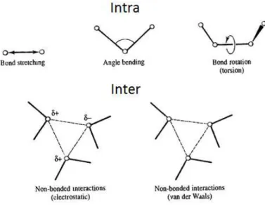
Figure 1.5 – Representation of the deferent types of interaction that occur intra and inter molecular level. ... 27

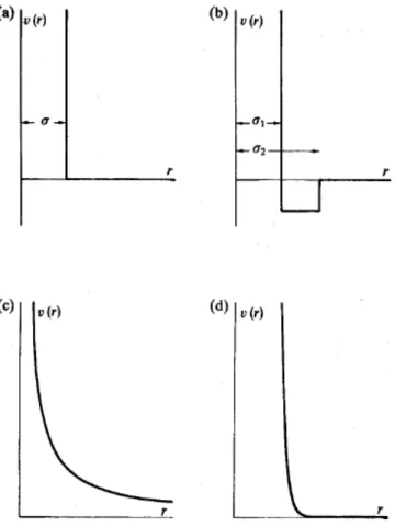
Figure 1.6 – a)The hard-sphere potential, b)The square-well potential; c and d) The soft-sphere potential with different repulsion parameter (v), whit v(c)>v(d). Adapted from [29] ... 28

Figure 1.7 – Representation of a typical 12-6 Lennard Jones potential. ... 29

Figure 1.8 – Schematic representation of and Bond Torsion. Adapted from [30] ... 30

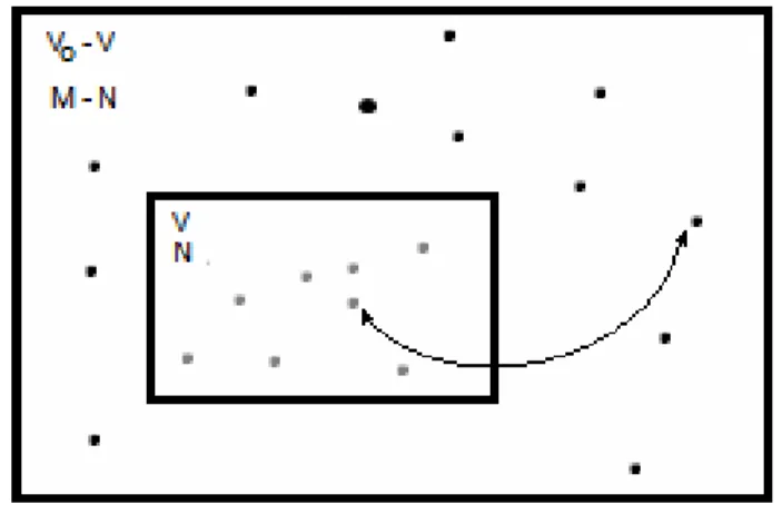
Figure 1.9 – Schetimatic GCMC simulation of an insertion/deletion move. Ideal gas (M – N particles, volume V0 – V) can exchange particle whit a N-particle system (volume V) ... 36

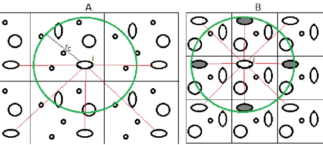
Figure 1.10 – Representation the simulated box and their naboring boxes. In A the cut radius is smaller than the simulation box length; In B the cut radius is larger than the simulation box length 41 Figure 1.11 – Representation of SWNT at the left and of a MWNT at the right. Adapted from [45] . 43 Figure 1.12 – Scheme of and hexagon grid structure. Adapted from [47] ... 44

Figure 1.13 – (a) SWNT armchair, (b) SWNT zigzag e (c) SWNT quiral. Adapted from [46] ... 45

Figure 1.14 – Image of Scanning electron microscopy (SEM) of nanotubos a) Blocks of synthesize nanotubos on plate whit pores size, 250x250 μm, b) 38x38 μm. c) Lateral vision of the towers. d) Tower’s top e) SEM image showing the carbon nanotubes perfect aliened. f) Image of a transmission electron microscope (TEM) of nanotubos growth in several towers g). Adapted from [46] ... 46

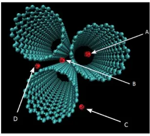
Figure 1.15 – Red dots represented possible sites for adsorption in a group of nanotubes. ... 48

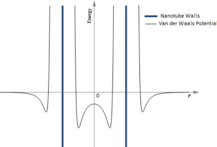
Figure 1.16 – Representation of the Lennad Jones potential, in and out of the nanotube walls. ... 49

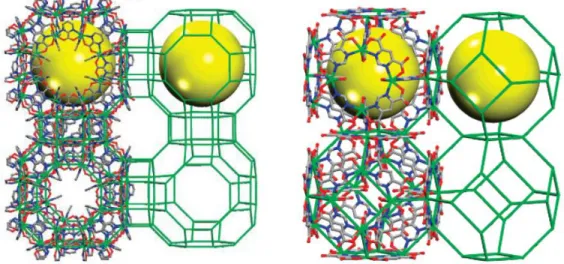
Figure 1.17 – Single-crystal structure of rho-ZMOF (left) and sod-ZMOF (right). Hydrogen atoms and quest molecules are omitted for clarity. In - green, C - gray, N - blue, O - red. The yellow sphere represents the largest sphere that can be fit inside the cage, considering the van der Waals radii. Adapted from the American Chemical Society. Adapted from [86] ... 52

Figure 1.18 – Different type of organic linker. ... 53

Figure 1.19 – Representation the main structure of the UiO-67Zr. ... 53

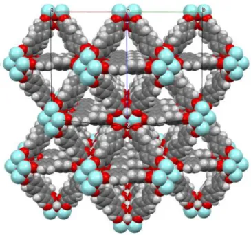
Figure 1.20 – Representation of eight molecules of UiO-67Zr. ... 54

XXI

List of Tables

1

1 Background

1.1 Motivation

The continue increase of the energy demand and its effect on the world economy and environment are the main impulse for new studies and technologies. A sustainable and efficient process to harvest and sustain many forms of energy is fundamental to ensure the reliable and sustainable use of such new technologies. Nowadays many forms of energy can be used; they can be divided into two major classes: non-renewable energy sources and renewable energies sources. Until now the use of non-renewable energy sources has been very important for human development, due to their high energy density and the innumerous sub-products that can be obtained from them. However, the improper consumption of such forms of energy results in severe effects on the environment.

The burning of non-renewable fuels, such oil and its derivatives, results in tremendous amounts of carbon dioxide released to the atmosphere. Carbon dioxide absorbs easily the infrared radiation and thus contributes intensely to the greenhouse effects. It is clear that the proper choice of the type of fuel that can be used has a significant impact on the environment. Today many developed countries are adopting new policies in term of the amounts of carbon dioxide released.

The investment that is made on new technologies depends on the world economics and for that, technologies must be not only be efficient and less polluting but also economically viable [1].

The large reserves of natural gas, as well as the increasing interest in shale gas, and the fact that methane is considered and as an environmentally friendly fuel gas, is leading investors to bet on this type of fuel. Although methane production derives from nonrenewable energy sources, it emits much less carbon dioxide than liquid hydrocarbon fuels due to his high hydrogen/carbon ratio. The problem with methane is that it is a gaseous fuel and thus it is not easy to store it compactly and safely [2].

2

The development of new adsorbent materials, such as metal organic frameworks and carbon nanotubes, has originated many new adsorbents with different properties, which can be tailored to enhance their adsorption capacity and/or selectivity. The metal–organic frameworks have recently shown a strong research interest because of their rigid structures, large pore volumes, tunable pore sizes, large surface areas, and potential applications as novel adsorbents. Regarding the adsorption properties of the carbon nanotubes, their large surface areas and 1-D nature of their porous topology are setting the carbon nanotubes as a very promising adsorbent. [4] [5]

The experimental study of numerous porous materials can be time consuming and many times not cost effective. In order to overcome that handicap, computer simulation has been steadily developed and matured since the 1950’s, with the aim of replacing many experiments with accurate precision. For the study of adsorption, computer simulation offers many possibilities, since it is easy to experiment with many materials under different thermodynamic conditions.

To properly perform a computer simulation it is important to understand what is a computer simulation, how it works, and what method it is based on.

The study and work in thermodynamics made by many scientists since

sixteen century,

proved to be one of the most importance of all fields of science. Driven by the invention of the steam engine, it represents an important role in the history of physics, chemistry, classical mechanics and quantum mechanics, which allow making great discoveries that have change the world for what we know today. Therefore it is of most importance to understand the basis of the innumerous concepts that forms thermodynamics, facilitating the conjugation between the real world changes and its mathematical expression.

In this thesis the comprehension of thermodynamics will focus on the process of adsorption and the variables that govern this phenomenon. Their mathematical expression will able us to compute data and simulate adsorption, not only for a single adsorbent and adsorbate, but for a variable range of compounds. This is a real advantage compared to the experimental process, where the measurement of an isotherm is a time consuming task whereas its simulation only takes a fraction of it. So, in order to obtain a very good molecular simulation it is fundamental to have all terms correctly and understand how they will change with the variation of some parameters, such as: temperature; pressure; volume and number of particles in the system under study.

3

We consider the concept called Ergodicity, introduced by Boltzmann in 1887 and developed later by J.Willard Gibbs in 1902, where it is proposed that the mean of a certain property in space, regarding to the position in the system, is equal to the average of that property over time. For this matter it is possible to obtain statistical averaged properties by two different methods: one that computes averages over the simulated time, called Molecular Dynamics, and other that computes averages over a number of trial configurations of the system, called Monte Carlo simulation. Both have advantages and disadvantages; the one selected for a particular problem depends on the type of properties that we wish to compute and the time of the computation.

Conjoining the work done by Boltzmann and Gibbs in statistical thermodynamics and using some slapping methods it is possible, choosing the proper force field for each single molecule and the excitations that will occur in the neighborhood of these molecules, to find the lower energy level in a system and consequently the equilibrium, being this, the basis to the Monte Carlo (MC) simulation.

4

1.2 Fundamental Concepts in Thermodynamics

The thermodynamics name result in the combinations of two Greek word, therm and dynamis, heat and power respectively. It’s the science of energy where the temperature has a very important role. Emerging after the construction of the steam engines, many developer and scientists, such as Thomas Savery, Thomas Newcomen, Carnot, Rankine, Clausius, Kelvin, Gibbs, contribute to the formulation of thermodynamic principles that describe the conservation and conversion of energy. For this, many formulations, concepts and laws where introduced to explain a field of science that is based entirely on logic, and so, it is essentially to understand the most important definitions.

1.2.1 Systems

In thermodynamics a system is a part of the physical universe and it is delimited by a specified boundary. In order to make good predictions on the thermodynamics properties of the system, the system must be composed by a large number of particles, in the order of the 1023 - 1025. Because thermodynamics is an average of the microscopic properties a large number of particles have a benefic effect of the statistical values, there for is pre-establish that a number of particles N, must be higher than 1015 order.

A thermodynamic system has a well-defined geometric volume and its boundaries separates the inside from the outside, that system can also be continuous, discontinuous, or discrete. In the simulation performed we use a simulation box that corresponds to a part of a discrete system. The simulation tool uses then the data from that box and replicates that box into others that will form the surrounding environment, simulating then a discrete system.

In any case, a thermodynamics system is a very dynamic system and so there are innumerous degrees of freedom that it should take into account. Because of that, determination of the properties becomes a very stiff process and for that, there is the need to characterize ideals systems in various types. Mainly a system can be divided into three major types: isolated system; close system; open system.

5

Close systems are the systems that can change energy with the exterior but not matter. So the only thing that remains constant is the number of particles.

Open systems allow the exchange of matter and energy. These systems are the most related to real exchanges and therefor heat, volume and the number of particles are not constant. For that reason, predicting their thermodynamics properties is a more complex process. Classical thermodynamics deals especially with close systems, for open systems statistical thermodynamics is the most suitable.

1.2.2 Thermodynamic properties

Thermodynamics properties consist in the physical or chemical attributes that specify the macroscopic characteristic properties of a system. These macroscopic properties result from the statistical averages of the observable microscopic coordinates of motion and position, being that motion set by a momentum or kinetic energy and position by potential energy.

It is possible to define two types of thermodynamics properties: intensive and extensive properties. Extensive properties are dependent on the size of the quantity of matter in a system. Mass, energy, entropy are just a few examples, and such properties are additives. On the other hand, properties like temperature, pressure and others are intensive properties and are not dependent on the size of the quantity of matter in a system, and some, can be express as derivatives of extensive properties. Thermodynamics properties can also be conservative and non-conservative. Conservative properties in isolated system do not change, that also means that besides the path that a certain properties takes to point A to point B, and then returns to point A by other path is initial values will remains de same. Properties like energy, mass, momentum, and others, are conservative properties. A very simple example of a conservative property is the potential energy, where it value only depends on the height of the object and not the path that he made to get there. Non-conservative properties change their energy to the system as they move along the point A to the point B, that energy is converted into a form which can’t be used by these properties again one example is the work done by friction.

6

1.2.3 Energy

Energy is a conservative and extensive property of every system and it can be transferred between systems by the flow of heat and mass or by work exerted by one system on the other. There are also different forms of energy, the most common being internal, potential, kinetic. Depending of the type of the system that is under study, it is possible to obtain different types of variations of energy in the system. In order to fully calculate the parameter of interests, it is more useful to measure the variation of the energy than the total energy of the system. That calculation is done taking into account a reference state and so, the final energy of the system after a perturbation is the sum of the reference state plus the variations that occur in the systems. It is important to refer, that to occur a variation in the system some energy must be spent doing work or to transfer heat; by definition this energy is called free energy of the system. The variations of energy depend not only of the type of the system and boundaries, but also depend of the different types of forms. When the free energy reaches a minimum value, the the system is under thermodynamic equilibrium.

1.2.4 Boundaries

Systems are separated from the exterior by a boundary and so all the work and heat done to the systems have to cross that boundary. In order to simplify the process and diminish the degrees of freedom it is establish some restrains on these boundaries. The types of boundaries also have a very important role to the determination of the thermodynamics properties, and depending of the types of boundaries that are in study it’s possible to relate them to real working conditions. So in order to do that, it’s used the extensive and intensive thermodynamics properties present earlier, given them some restrain and creating then, the various types of boundaries for each types of system. Next, its present the major types of boundaries and how they affect the change of the thermodynamics properties.

1.2.4.1 Adiabatic Boundaries

Adiabatic Boundaries are restrictive only to the change of heat and so any of the other major properties aren’t constant.

7

1.2.4.2 Rigid Boundaries

Rigid Boundaries don’t allow the variation of the volume, therefor the introduction of particles in the systems will result in the increase of pressure.

(V = const, P ≠ const, Q ≠ const, S ≠ const, U ≠ const, N ≠ const T ≠ const,)

1.2.4.3 Moving Boundaries

Moving Boundaries basically are the reverse of a rigid Boundary. They don’t allow the variation of pressure and therefor the introduction of particles in the systems will result in the increase of volume.

(P = const, V ≠ const, Q ≠ const, S ≠ const, U ≠ const, N ≠ const, T ≠ const,)

Choosing then the right system and the right boundaries, it’s possible to represent correctly the real system in study and construct the correct mathematical expression for the free energy. However not only the characterization of the system and is boundaries it’s enough and for that reason it was necessary to formulate the laws of thermodynamics.

The choice of the types of boundaries will depend of the conditions of experimental work that is being done. In chemistry it’s easier to maintain the system at constant pressure than the volume and for that reason it’s often chosen moveable boundaries.

1.2.5 Laws of thermodynamics

8

1.2.5.1 The zeroth law of thermodynamics

The zeroth law, allow to build up a universal temperature scale and it states that if a system A is in equilibrium with system B, and if system B is in equilibrium with system C, then system A is in equilibrium with system C. If a system is in thermal equilibrium, it is assumed that the energy is distributed universally all over the volume. Also state that if the energy of a system increases the temperature of that system also increases

1.2.5.2 The first law of thermodynamics

Energy is defining as a conservative force so depends only on the initial and final states, not on the path between these states and so it’s is possible to arrange a mathematical expressing to the internal energy. The use of a cyclic integral assures, Eq. 1.1, that when a specific variable returns to the initial state their value will be the same. This condition ensures the conservation of energy in the universe. [8]

∮ 𝑼 = 𝟎

Eq. 1.1

The first law considers then, that the variation of the internal energy depends on the work done by the environment into the system, by definition it’s a positive value and, depends on the heat receive into the system, that by definition it’s is a positive value as well.

𝒅𝑼 = 𝒅𝑸 + 𝒅𝑾

Eq. 1.2

In general, the term δW represents all different forms of work, being the most commonly used the work done by compression, by surface deformations and by and chemical work (µdni).

𝜹𝑾 = −𝑷𝒅𝑽 + 𝝈𝒅𝑨 + µ𝒅𝒏𝒊

Eq. 1.3

9

1.2.5.3 The second law of thermodynamics

The second law results of the empirical observation of some process that occurs in nature, and it’s very important to define the direction of the flow of energy and when it’s stops. This, states that in a process containing two systems, the flow of energy will goes in the direction of the hotter system to the colder system until they reach the equilibrium. To express this occurrence correctly, it was needed to formulate a new property named entropy. This property was introduced by Carnot in 1824 and further developed by Clausius and Kelvin in mid-1850. [7]

1.2.6 Entropy

Whit the formulation of the second law and whit the use of statistical mechanics it was possible to define Entropy (S). This property is a non-conserved and extensive property of a system in any state and its value is part of the state of the system. The change of energy in the system will results then in the destruction of creation of entropy.

It’s often said that entropy is a disorder of a system however this definition it’s not the best one to express this property properly. So entropy is actually a function of a natural logarithm of the total multiplicity of states (Ω). Analyzing the probability of the multiplicity of given state, it is observed that the most likely value is one that has a higher multiplicity for a given state and so the entropy will have a maximum value when it’s in equilibrium. That probability is depend of the quantity of energy in the system and is increase will allow reaching higher states of energy.

The expression of the entropy related to the multiplicity of states was formulated by Boltzmann.

𝑆 ≡ 𝑘

𝐵

∗ ln Ω

𝑇 Eq. 1.4

Where kB is the Boltzmann constant and represents the ratio of the ideal gas constant with Avogadro’s number (kB=1.38066x10-23 J/K), this constant give the dimension requires and the use of the natural logarithm allow a value to Ω more suitable.

Analyzing then the dimensions of the variation of the entropy in function of the variation of the internal energy (U in Joules), it is possible to arrange the following function:

(

_𝜹𝑼𝜹𝑺

)

𝑽,𝑵

=

𝟏

10

Writing the entropy as a function of the internal energy and temperature gives:

𝒅𝑺 =

𝒅𝑼_𝑻 Eq. 1.6

Considering the first law and assuming that volume is constant i.e. the work done in the system is equal to zero, the expression of the entropy takes the most common way.

𝒅𝑺 =

𝒅𝑸_𝑻 Eq. 1.7

1.2.7 Thermodynamic Potentials

Thermodynamic potentials are state functions of energy that differ according to different properties. The types of property chosen to represent the system have a significant and different impact and therefore different types of energy can be obtained. Those properties can be a set of extensive and intensive properties and with the help of the Maxwell relation and the Legendre transforms it is possible to obtain the different types of energy, and expressions for different experimental conditions, such as changes in volume, temperature, pressure, composition.

The most common thermodynamic potentials are the Internal Energy (U), Enthalpy (H), the free Helmholtz Energy (F) and the free Gibbs Energy (G).

1.2.7.1 Internal Energy (U)

Internal energy represents the energy needed to create the system. As previously present in the definition of the first law of thermodynamics, energy is the sum of the heat and work done in a closed system. If the system is open to material, then it must be consider the energy of particles added. Combining the second law, obtains the expression to internal energy in function of extensive variables as volume, entropy, and number of interchange in chemical species. [8]

𝒅𝑼 = 𝑻𝒅𝑺 − 𝑷𝒅𝑽 + ∑ µ𝒅𝒏𝒊

𝒊 Eq. 1.8

Considering that entropy and volume remained constant:

µ

𝒊

= (

_𝜹𝒏𝒊𝜹𝑼

)

_{𝑺,𝑽,𝒏} 𝒊

Eq. 1.9

11

In classical molecular simulation the total interaction potential is considered to be the additive interactions with other atoms on the same molecule (bonded, bending angles, torsion, improper torsion, and intramolecular nonbonded terms) and interactions with other molecules (intermolecular nonbonded terms).

𝑼(𝒓) = 𝑼

𝒏𝒐𝒏 𝒃𝒐𝒏𝒅

+ 𝑼

𝒃𝒐𝒏𝒅

+ 𝑼

𝒃𝒆𝒏𝒅

+ 𝑼

𝒕𝒐𝒓𝒔𝒊𝒐𝒏

+ 𝑼

𝒊𝒎𝒑.𝒕𝒐𝒓𝒔𝒊𝒐𝒏

+ 𝜺

𝑲 Eq. 1.10

1.2.7.2 Free Helmholtz Energy (F)

The free Helmholtz energy considers that if a system created with rigid boundaries, where no variations on volume occur, in an environment with a certain temperature, higher than the temperature of the system created, it’s possible to gain some energy from the environment and so the amount of energy need to create a system will be less. Other possible way to obtain this is considering that we have a Legendre transformation on the variation of the internal energy, replacing in the correct way the entropy by the temperature. The Helmholtz free energy can be written as:

𝑭 = 𝑼 − 𝑻𝑺

Eq. 1.11

Taking the direct differential on F, and replace dU, obtained:

𝒅𝑭 = 𝑻𝒅𝑺 − 𝑷𝒅𝑽 + ∑ µ𝒅𝒏𝒊

_𝒊

− 𝑻𝒅𝑺 − 𝑺𝒅𝑻

Eq. 1.12

𝒅𝑭 = −𝑺𝒅𝑻 − 𝑷𝒅𝑽 + ∑ µ𝒅𝒏𝒊

𝒊 Eq. 1.13

Considering that temperature and volume remained constant:

µ

𝒊

= (

_𝜹𝒏𝒊𝜹𝑭

)

_{𝑻,𝑽,𝒏𝒊} Eq. 1.14

1.2.7.3 Enthalpy (H)

The enthalpy consists in the internal energy plus the energy necessary to create room for the system in the environment, so in these conditions there are no changes in the pressure and the boundaries are moveable. To obtain this type of energy with the Legendre transformation it is needed to replace the volume by the pressure as an independent variable. The enthalpy can be written as

𝑯 = 𝑼 − (−𝑷𝑽)

Eq. 1.15

Note in this case, the variations of the work done is negative, this appends because is the systems that is making work to the environment and not the contrary.

12

𝒅𝑯 = 𝑻𝒅𝑺 − 𝑷𝒅𝑽 + ∑ µ𝒅𝒏𝒊

𝒊

+ 𝑷𝒅𝑽 + 𝑽𝒅𝑷

Eq. 1.16

𝒅𝑯 = 𝑻𝒅𝑺 + 𝑽𝒅𝑷 + ∑ µ𝒅𝒏𝒊

𝒊 Eq. 1.17

Considering that entropy and volume remained constant:

µ

𝒊

= (

_𝜹𝒏𝒊𝜹𝑯

)

_{𝑺,𝑽,𝒏} 𝒊

Eq. 1.18

1.2.7.4 Free Gibbs Energy (G)

The free Gibbs energy considers that if a system crated whit moveable boundaries, where no variations on the pressure occur, in an environment whit a certain temperature higher than the temperature of the system created, it’s possible to gain some energy from the environment and, because the system needs to create room for itself this will consist in an energy loss as well. To obtain the free Gibbs energy with the Legendre transformation it is needed to replace the volume by the pressure as an independent variable and the entropy by the temperature. The free Gibbs energy can be written as:

𝑮 = 𝑯 − 𝑻𝑺

Eq. 1.19

𝑮 = 𝑼 + 𝑷𝑽 − 𝑻𝑺

Eq. 1.20

Taking the direct differential on G, and replace dU, obtained:

𝒅𝑮 = 𝑻𝒅𝑺 − 𝑷𝒅𝑽 + ∑ µ𝒅𝒏𝒊

𝒊

+ 𝑷𝒅𝑽 + 𝑽𝒅𝑷 − 𝑻𝒅𝑺 − 𝑺𝒅𝑻

Eq. 1.21

𝒅𝑮 = 𝑽𝒅𝑷 − 𝑺𝒅𝑻 + ∑ µ𝒅𝒏𝒊

𝒊 Eq. 1.22

Experimentally in chemistry it is easier to obtain thermodynamic data from variables that are easy to measure and control; these variables are the temperature and pressure. For this reason, in chemistry the free Gibbs energy is the most interesting form of energy to calculate. Considering the pressure and volume constant: [7] [9]

µ

𝒊

= (

_𝜹𝒏𝒊𝜹𝑮

)

_{𝑷,𝑻,𝒏} 𝒊

13

1.2.8 Ensembles

Ensembles are different conditions imposed on a system, and are developed in the field of statistical thermodynamics, they are particular useful when computing a system with a large number of particles, making the calculation performed much easier.

In statistical thermodynamics, the collection of possible states dependable of some constraints is referred to an ensemble of states. Depending on the constraints, special names are given to these ensembles.

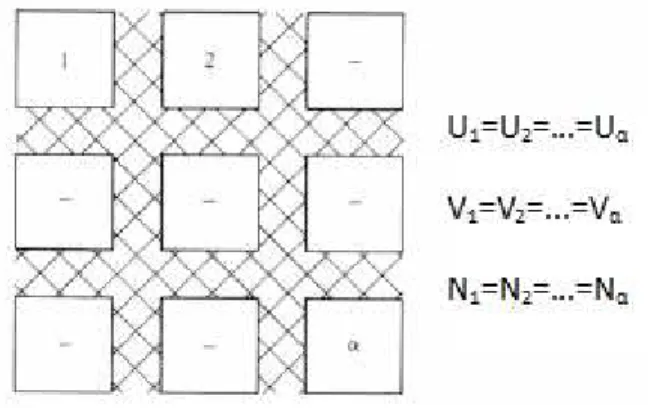
1.2.8.1 Microcanonical (U,V,N)

This ensemble considers an isolated system with rigid boundaries, where the total energy, the volume and the number of particles in the box remain constant. A micro-canonical ensemble is an assembly of innumerous copies of an isolated system where they have all the same energy.

Since isolated systems are difficult to realize in practice, the microcanonical ensemble is not often used. The image below demonstrated the many copies of the system separated from each other.

Figure 1.1 –Microcaninical ensemble. Systems 1 trough α, are isolated from each other. Adapted from [10]

1.2.8.2 Canonical (N,V,T)

14

Unlike the microcanonical ensemble where there isn’t any change in the energy of the system and consequently no changes in ground state, in the canonical ensemble is necessary taking into account the variation of energy and find the ground state at equilibrium. That is done according to the metropolis scheme, where a random walk is constructed trough a region of space. That random walk is constructed through trial moves, in order to find a lower energy in the system. The trial moves are done randomly, by sampling methods and when one generates an energy level higher than the previous that trial move is reject.

Figure 1.2 –Canonical ensemble. Systems 1 trough α, are complete closed from each other. Adapted from [10]

1.2.8.3 Grand canonical (µ, V, T)

This ensemble considers an open system with rigid boundaries where the temperature, volume and chemical potential remain constant. For this type of ensemble it is possible to have changes of heat as well changes in the number of particles.

Similar to the Canonical ensembles, the Grand canonical ensemble uses a modified metropolis method to compute thermodynamics averages, where the difference it is in the variables used. Since the number of particles is deeply related with the chemical potential it is possible to shift a variable to another, and so for a particular chemical potential imposed, in equilibrium, will be a specific number of particles in the simulation box.

15

This type of ensemble is the ideal one when simulating systems that require adding or removing some particles, for example the study of adsorption phenomena or phase transitions. For that reason this will be the type of ensemble used in the simulation performed.

1.3 Adsorption phenomenon

Adsorption is the phenomenon of accumulation of a gas or liquid on a surface of a solid or liquid. By definition the component being adsorbed is call adsorbate and the solid is called adsorbent. This phenomenon takes place at the presence of two distinguishesD phases where at the boundaries the accumulation of particles occurs.

Adsorption has been used since the ancient Egyptian and Sumerians but its study only started with the observations carried by Scheele in 1773, experimenting adsorptions of gases in charcoal and clays.

For large scales process, major development were made in systems that have in is present two distinguish phase, solid-gas and solid-liquid. Many processes were driven by the developments made and today many applications for adsorption can be found, for example, separation processes of gaseous and liquid mixtures, heterogeneous catalysis, chemical analyses, biological process, such drug delivery, separation and purification of gases.

Adsorption process is recognized as the most efficient, promising and widely used essentially because of its simplicity, economically viable and technically feasible. Despite of is abundant use in large industries, the biggest barrier of its application by the industries is the cost-prohibitive adsorbent and difficulties associated with regeneration. [11]

In the effort to explore novel adsorbents and to find the ideal adsorption material, it is essential to establish the most appropriate adsorption equilibrium correlation, which is indispensable for reliable prediction of adsorption parameters and quantitative comparison of adsorbent behavior for different adsorbent types. So, in order to analyzing correctly the capabilities of adsorption of a material it’s is fundamental to know is equilibrium curves, being that curves obtain at different conditions. Like, constant volume the isochoric curve, at constant pressures the isobaric curve and the most usual equilibrium curve at constant temperature the isotherm curve.

Theses curves are important tools for describing adsorption phenomena that occur at various types of interfaces, allowing characterize the types of porous of the material in study. Adsorption may occur by two distinguish types, physical or chemical, where the type of bonding between the adsorbate and the adsorbent depend the conditions of the system.

16

Physical adsorption or physisorption is a type of adsorption in which the adsorbate adheres to the surface mainly through Van der Waals interactions. This requires much less energy comparing to the chemisorption so the process of physisorption is a fast process, reversible and can form a multiplayer.

1.3.1 Adsorption equilibrium

Adsorption equilibrium is established when the chemical potential of the adsorbate in the bulk is equal to the chemical potential of the adsorbate in the adsorbent, whereas a ratio between the amount adsorbed with the remaining in the solution remains constant. There are many types of isotherm models that describe a variety of adsorbents: Langmuir; Freundlich; Sips; Brunauer– Emmett–Teller (BET), and many other. [12]

1.3.1.1 Langmuir isotherm model

Langmuir adsorption isotherm was originally developed to describe gas–solid-phase adsorption in activated carbon. In its formulation, the model assumes monolayer adsorption, having then a finite number of sites to adsorbed, this model can be also used for adsorbents where occurs chemisorption. Langmuir isotherm refers to homogeneous adsorption, which each molecule possess constant enthalpies and sorption activation energy (all sites possess equal affinity for the adsorbate).

Considering the fractional surface coverage or fractional filling of the micropore θ is the reason of the quantities adsorbed (q) over the quantity of saturation (qS) and assuming a perfect gas, it’s possible to related the adsorption rate with the desorption, obtaining the expression to the Langmuit model. [11] [13]

Adsorption:

𝒅𝜽

𝒅𝒕

= 𝒌

𝒂

𝑷 ∗ (𝟏 − 𝜽)

Eq. 1.24 Desorption:

𝒅𝜽

𝒅𝒕

= 𝒌

𝒅

∗ 𝜽

Eq. 1.25 In equilibrium both rates are equal, obtaining:

𝜽 =

_{𝟏+𝑲𝑷}𝑲𝑷 Eq. 1.26

With:

𝜽 =

_𝒒𝑺𝒒 Eq. 1.27

17

𝑲 =

𝒌𝒂

𝒌𝒅 Eq. 1.28

The linearization of the expression 1.26, leads to: 𝟏

𝒒

=

𝟏 𝒒𝑺

+

𝟏 𝒒𝑺∗𝑲

∗

𝟏

𝑷 Eq. 1.29

1.3.1.2 Freundlich isotherm model

Freundlich isotherm is the earliest known relationship describing the non-ideal and reversible adsorption and can be applied to multilayer formation, with non-uniform distribution of adsorption, heat and affinities over the heterogeneous surface. At the beginning of the study of these models, it was proved that the ratio of the adsorbate for a given mass of adsorbent wasn’t a constant at different solution concentrations.

The adsorption in this models is represent by the summation of adsorption on all sites, each having different bond energy, where the stronger sites are occupied first until adsorption energy exponentially decreased, completing the adsorption process. The Freundlich isotherm can be represented by the fouling expression: [13]

𝒒 = 𝑲

𝑳

∗ 𝑷

𝟏

𝜼 _{Eq. 1.30}

Where KL is the Freundlich constant and 1/n depends on the linearity of the isotherm , varying between 0 and 1. These constants are related to adsorption capacity and adsorption efficiency, respectively.

Since the value of 1/n varies between 0 and 1, this models of isotherm maybe not the best to represent some systems, once at high pressures the value of q may surpass the quantity of saturation. The linear for of the Freundlich isotherm model can be represent by the following expression: [14] [11]

𝐥𝐧(𝒒) = 𝐥𝐧(𝑲

𝑳

) +

𝟏_𝒏

∗ 𝐥𝐧 (𝑷)

Eq. 1.31

1.3.1.3 Sips isotherm model

18

The expression to the Sips isotherm model can be obtained considering that at equilibrium, the rate of desorption is equal to the rate of adsorption. The n parameter could be regarded as the parameter characterizing the system heterogeneity being higher than 1, so:

Adsorption:

𝒅𝜽

𝒅𝒕

= 𝒌

𝒂

𝑷 ∗ (𝟏 − 𝜽)

𝒏 Eq. 1.32 Desorption:

𝒅𝜽

𝒅𝒕

= 𝒌

𝒅

∗ 𝜽

𝒏 Eq. 1.33 In equilibrium both rates are equal, obtaining:

𝜽 =

(𝑲𝑷)

𝟏 𝒏

𝟏+(𝑲𝑷)𝒏𝟏

Eq. 1.34

Regarding temperature dependence on the terms K an n, it’s have:

𝑲 = 𝑲

𝟎

𝒆

[ 𝑸

𝑹𝒈𝑻𝟎(𝑻𝟎𝑻−𝟏)] _{Eq. 1.35}

𝟏 𝒏

=

𝟏

𝒏𝟎

+ 𝜶 (𝟏 −

𝑻𝟎

𝑻

)

Eq. 1.36

Where the K0 is the affinity constant at a reference temperature, T0, n0 is the parameter n at the same reference temperature and α is a constant parameter. Rg is the ideal gas constant and Q is the heat of adsorption. [15]

1.3.1.4 BET isotherms

The Brunauer–Emmett–Teller (BET) isotherm was first introduced in the 1930s by Brunauer, Emmett and Teller is a theoretical equation, most widely applied in the gas–solid equilibrium systems. It was developed to derive multilayer adsorption systems with relative pressure ranges from 0.05 to 0.30

For the formulation of this isotherm it is consider Van-der-Waals forces, where each layer have a different quantity of energy, affecting the time and rate of absorption. Having then:

Adsorption into the ith _layer:

19

Desorption into the ith layer:

𝑹

𝒅𝒊

= 𝒌

𝒅𝒊

∗ 𝑺

𝒊

∗ 𝒆

− 𝑬𝒊

𝑹𝑻 Eq. 1.38

where Si is the surface area and P the pressure; ka and kd correspond to the adsorption and desorption constants.

In this model is important to differentiate the monolayer from the other layers that are form above, in order to conjugate both expressions, Eq. 1.37 and Eq. 1.38, at equilibrium and obtain a more generic form of the expression for the monolayer and the layers that follows after:

Having for monolayer:

𝒌

𝒂𝟏

. 𝑷. 𝑺

𝟎

= 𝒌

𝒅𝟏

. 𝑺

𝟏

. 𝒆

− 𝑬𝟏

𝑹𝑻 Eq. 1.39

And for the other layers a more generic for:

𝒌

𝒂𝒊+𝟏

. 𝑷. 𝑺

𝒊

= 𝒌

𝒅𝒊+𝟏

. 𝑺

𝒊+𝟏

. 𝒆

− 𝑬𝒊+𝟏

𝑹𝑻 Eq. 1.40

By definition at equilibrium:

𝒚 =

𝒌𝒂𝟏 𝒌_𝒅𝟏

. 𝒆

𝑬𝟏

𝑹𝑻

and

𝒙 = 𝑷 ∗

𝒌𝒅𝒏 𝒌𝒂𝒏

. 𝒆

𝑬𝑳

𝑹𝑻 with L>2

Eq. 1.41

Relating the energy with the surface area of the monolayer obtain an expression to the total area for each energy state. With that is possible to find an expression to the surface coverage (θ). Obtaining: [16] [17]

𝜽 =

𝑽𝒕𝒐𝒕𝒂𝒍 𝑽𝒎𝒐𝒏𝒐

=

(𝒄.𝑺𝟎.∑𝑳𝒊=𝟏𝒊.𝒙𝒊) 𝑺𝟎.(𝟏+𝒄.∑𝑳𝒊=𝟏𝒊.𝒙𝒊)

Eq. 1.42

Being:

𝒄 = 𝒚/𝒙

Eq. 1.43

Rearranging the expression into a more suitable form, obtain: 𝟏

𝑽𝒕𝒐𝒕𝒂𝒍

. (

𝒙 𝟏−𝒙

) =

𝟏 𝒄.𝑽𝒎𝒐𝒏𝒐

+

(𝒄−𝟏) 𝒄

.

𝟏

𝑽𝒎𝒐𝒏𝒐

. 𝒙

Eq. 1.44 Substituting:

𝒙 =

_𝒑𝒑

20

Finally arrive at the famous BET isotherm in the common form:

𝟏 𝑽𝒕𝒐𝒕𝒂𝒍

. (

𝒑 𝒑𝟎−𝒑

) =

𝟏 𝒄.𝑽𝒎𝒐𝒏𝒐

+

(𝒄−𝟏) 𝒄

.

𝟏 𝑽𝒎𝒐𝒏𝒐

.

𝒑

𝒑𝟎 Eq. 1.46

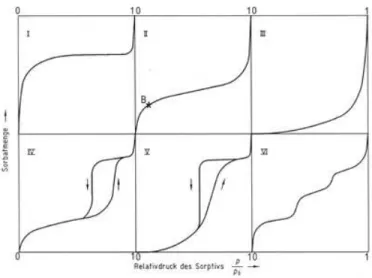
Combining some of this simple models, such as Langmuir and BET, and using their capability to express different types of phenomenon that occur during adsorption, other models where construct and improved to obtain other information and to express correctly the isotherm of different types of porous. Isotherm can be represented in six different types: [11] [12] [18] [19] [20]

Figure 1.4 – The six types of adsorption isotherms, as classified by IUPAC. Specific amount adsorbed versus relative pressure P/P0, where P0 is the saturation vapor pressure. Adapted from [18]

Type I: Represent adsorption on microspores or adsorption in the monolayer. The rapid increases of the curve represent a rapid filling of the pores, enhanced on the microspores, by the overlapping of the interaction energy of the neighboring walls.

Type II: These types of isotherm are observed in multilayered adsorption on non-porous solids as well as microspores. Where point B represents the quantity on the monolayer of a microspore. Type III: Represent adsorption on non-porous or macrospores solids, where are weak interactions gas-solid.

Type IV: The initial part of the isotherm is attributed to monolayer and multilayer adsorption. It is also possible to observe a hysteresis loop, which is associated with capillary condensation, taking place in mesopores. In the simplest cases this type of isotherm are very similar to Types II.

Type V: This type of adsorption may occur in mesoporous or microporous solids, and similar to the Type III isotherm week forces gas-solid are associated to adsorption.

21

Despite of the existence of many models that represent a series of compounds and their properties, those depend on experimental data or the solution of integral equation very hard to solve and calculate, and so the use of alternative methods, facilitate not only in the time consumed but also provides different types of experiences that can be tested.

That only was possible whit the implementation of the virial formalism in 1974, by Steele, and turn out to be the turning point in adsorption study. The numerical values of the second, third and fourth two-dimensional virial coefficients give qualitative information on the interactions between adsorbed molecules and adsorption sites as well as on the interactions with other adsorbed molecules, and there value are regardless if the adsorbent surface is homogeneous or heterogeneous.

The big handicap of the methods that uses the virial formalism is the present of a distribution function in the coefficients, being that function very hard to get by simple numeric methods. Only with the power of molecular simulation that’s was possible to overcome some problems and obtained some results with very good precisions

Based directly on a microscopic model of the adsorption system, the computer simulation approach, both Monte Carlo as well as Molecular Dynamics, can provide then, an exact numerical solution of the model assumed. [12]

1.3.2 Adsorption Thermodynamics

In order to fully understand the adsorption phenomenon that occurs at surface of an adsorbent, it’s fundamental to not only have into consideration the kinetic approach but also the thermodynamics that govern that process. The result is the understanding of the forces that governs adsorption, the types of binding between molecules and the variation of the energy of the system whit the change of is conditions and types of particles. [15]

Since adsorption is a spontaneous process, changes in the total energy of the systems must be considered. That change occurs mostly due to the tendency of transition between molecules in different phases. That transitions result usually in a loss of entropy (ΔS < 0), once molecules that are in the gas phase have more degrees of freedom when comparing whit the ones that are adsorbed phase. Considering then a spontaneous process, it follows that adsorption must always be exothermic (ΔHads < 0) since:

𝚫𝐆

𝐚𝐝𝐬

= 𝚫𝑯

𝒂𝒅𝒔

− 𝑻𝚫𝑺

𝒂𝒅𝒔

< 𝟎

Eq. 1.47

22

Where ΔHads represents the variation of enthalpy when a differential amount of adsorbate changes from the gas phase to the adsorbed phase. To achieve the equilibrium, the system tends to move the particles in the direction of the lower free energy state. At constant temperature and pressure, the equilibrium its obtain when the rate of particles, that goes from the gas phase to the adsorbate phase, is equal to the rate of particles that goes from the adsorbate phase to the gas phase, and so the variable to have into account is the chemical potential, since it’s related whit the number of particles. The chemical potential in each phase is defined as: [22]

𝝁

𝒂

= (

𝜹𝑮_𝜹𝒏𝒂_𝒂

)

𝑻,𝑷

= −𝐬

𝒂

𝒅𝑻 + 𝒗

𝒂

𝒅𝑷

Eq. 1.49

𝝁

𝒈

= (

𝜹𝑮𝒈_𝜹𝒏𝒈

)

𝑻,𝑷

= −𝐬

𝒈

𝒅𝑻 + 𝒗

𝒈

𝒅𝑷

Eq. 1.50

Where si and vi are extensive properties of the systems:

𝒔

𝒊

= (

_𝜹𝒏𝒊𝜹𝑺𝒊

)

𝑻,𝑷

𝒗

𝒊

= (

𝜹𝑽𝒊

𝜹𝒏𝒊

)

_𝑻,𝑷 Eq. 1.51

When equilibrium is reached, the chemical potential of the gas phase and the adsorbed phase are equal, since:

𝒅𝑮 = (𝝁

𝒂

− 𝝁

𝒈

)𝒅𝒏

𝒂

= 𝟎

Eq. 1.52

𝝁

𝒂

= 𝝁

𝒈 Eq. 1.53

−𝐬

𝒂

𝒅𝑻 + 𝒗

𝒂

𝒅𝑷

=

−𝐬

𝒈

𝒅𝑻 + 𝒗

𝒈

𝒅𝑷

Eq. 1.54

Taking the total derivative of temperature and pressure, on the previous equation, obtained the classic Clausius-Clapeyron relation:

𝒅𝑷 𝒅𝑻

=

𝒔𝒂−𝒔𝒈

𝒗𝒂−𝒗𝒈 Eq. 1.55

Considering that the volume of the gas phase is much larger than the adsorbed, this approximation is taken:

𝑣

𝑔

− 𝑣

𝑎

≈ 𝑣

𝑔

And so: 𝒅𝑷 𝒅𝑻

=

𝒔𝒈−𝒔𝒂

𝒗𝒈

= −(𝒔

𝒂

− 𝒔

𝒈

)𝝆

𝒈

= −𝚫𝑺

𝒂𝒅𝒔

∗ 𝝆

𝒈 Eq. 1.56 Leading to:

23

At equilibrium, the corresponding change in enthalpy upon adsorption is:

𝚫𝐇

𝐚𝐝𝐬

(𝒏

𝒂

) = 𝐓 ∗ 𝚫𝑺

𝒂𝒅𝒔

(𝒏

𝒂

) = −𝑻 ∗

𝒅𝑷_𝒅𝑻

∗ 𝝆

𝒈−𝟏 Eq. 1.58

Considering the ideal gas equation:

𝝆

𝒈

=

_𝑽𝒈𝒏𝒈

=

_𝑹𝑻𝑷 Eq. 1.59

𝚫𝐇

𝐚𝐝𝐬

(𝒏

𝒂

) = −

𝑹𝑻 𝟐 𝑷

∗ (

𝒅𝑷

𝒅𝑻

)

_𝒏𝒂 Eq. 1.60

Rearranging in the van’t Hoff form obtained:

𝚫𝐇

𝐚𝐝𝐬

(𝒏

𝒂

) = 𝐑 ∗ (

𝒅𝒍𝒏 𝑷_𝒅(𝟏 𝑻)

)

𝒏𝒂

Eq. 1.61

The isosteric heat of adsorption Qst (kJ/mol), a commonly reported thermodynamic quantity, is given as a positive value:

𝐐

𝐬𝐭

= −𝚫𝐇

𝐚𝐝𝐬

(𝒏

𝒂

) = −𝐑 ∗ (

𝒅𝒍𝒏 𝑷_𝒅(𝟏 𝑻)

)

𝒏𝒂

Eq. 1.62

1.3.2.1 Isosteric heat of adsorption

The decisive quantities when studying the adsorption process are the heat of adsorption, its coverage dependence on lateral particle–particle interactions, the kind and number of binding states and the nature of the surface of the adsorbent. The most relevant thermodynamic variable to describe the heat effects during the adsorption process is the differential isosteric heat of adsorption Qst, (kJ mol-1), that represents the energy difference between the state of the system before and after the adsorption for a differential amount of adsorbate on the adsorbent surface. It’s also need to have into account is the electrostatics nature of some molecules.

For nonpolar molecules the heat of sorption is generally almost constant for low coverage, however it’s shown a slightly increase as the coverage rises until reach saturation. That effect is often ascribed to the effect of intermolecular attraction. For the case of polar molecules, the heat sorption tends to decrease due to the power of polarization power. [23]

24

There are many methods that can be used to estimate the isosteric heat, one frequently used is to measure various adsorption isotherms and to plot the data under the form of an isosteric plot. Another option is to fit the isotherm data to a temperature dependent adsorption model and then to derive the heat of adsorption by applying the Clausius-Clapeyron equation to the isotherm model. Two isotherm models that are usually used for this purpose are the Sips and Toth models. It is worth noting that the Sips models equation is not valid at very low pressure because it does not possess the correct Henry -aw type behavior. To proper calculate and represent those values, the Toth models is the most appropriated since this model describes well many systems with sub-monolayer coverage. [25] [23] [22] [15] [13]

1.3.2.2

Henry’s Law

The Henry’s Law, describe the system in a very simplest way, where it’s used to describe the adsorption phenomenon at low occupancy. For very low pressures, at constant temperature, the relation between the pressure and the amount adsorbed can be express in the linear form, being the value of the slope the Henry constant. That value gives an insight of the affinity adsorbent and adsorbate, and gives also the possibility to compare the affinity of the adsorbent whit different types of adsorbates. If the chemical potential is sufficiently low, the loading q is proportional to the Henry coefficient KH and the pressure and the henry constant can be obtain by the flowing expression.

𝒒 = 𝑲

𝑯

. 𝑷

Eq. 1.63

Where KH is the henry constant, the q is the amount adsorbed and P is the pressure of the system. That equation can be easily obtained by a linear tendency line over the data obtain. [26]

For the last two decades the methods of molecular modeling of surface and interface phenomena have been widely developed. And with time other methods that are simplest and less time-consumers have been applied. The firsts, denominated as ‘atomistic computer modeling’, where based on the Schrodinger equation and in the advances made by Hartree FocK. Those type of models can be applied to any system regardless the availability of experimental data, obtaining properties prior to any synthesis and have a glimpse inside into materials behavior on the atomistic level.

25

1.4 Simulation Tools

The use of simulation tools to describe some complex systems have become essential in science since it discovery. Despite of being a complicated tool to understand and used, the combination of statistical mechanics and thermodynamics, the use of the correct force fields, the use of the second law of Newton and the implementation of some algorism, make the Computer Simulation a very precise and helpful tool.

It emerge essential during and after the Second World War, for code breaking and to develop nuclear weapons and only after computer became available for nonmilitary uses, in the early 1950’s, that has given a boom in this area. The first simulation performed in nonmilitary computer was carried out at the Los Alamos National Laboratories in United States by, Nicholas Metropolis, and many other scientists in 1952, on a computer called MANIAC (Mathematical Analyzer, Numerical Integrator, and Computer).

The use of computer simulation it only was possible with rapid increase of computer power and technology and today it’s possible to perform simulation on any ordinary computer thanks to the internet.

In theory it’s possible to simulate any system regardless of its size. However, even though of the remarkable computational power achieve today, the simulations performed goes around the number of atoms in the order of 106, representing fraction of a mole, in the order of 10-17. Despite of those values be very small, the objective when performing molecular simulation is to obtaining many types of information and properties, for example density, free energy, specific heat, viscosity and average structure. Simulation can be performing for many different purposes like drug design, protein engineering, environmental processes and materials science.

Although computer simulation have a very important role in science, it should have into considerer that simulation is by no means ideal. Simulation provides statistical estimates rather than exact characteristics and performance measures of the model. Thus, simulation results are subject to uncertainty and contain experimental errors. It´s also important to consider that, no matter how precise, accurate, and impressive, the information obtain is, that it’s only correct if the models is a valid representation of the system under study.

Computer simulation models can be classified in several ways:

 Static versus Dynamic Models: Where static models are the ones that are not time depend and therefor do not have a representation over the time. In contrast, dynamic models represent systems that evolve over time.

 Deterministic versus Stochastic Models: In a deterministic model, all mathematical and logical relationships between variables are fixed and not subject to uncertainty. They are often described by differential equations and solve by different numerical methods where a unique input leads to a unique output. In contrast, a model with at least one random input variable is called a stochastic model, where a unique input leads to different outputs.