The Quantitative Easing in China
Dapeng Nie
Dissertation submitted as partial requirement for the conferral of Master in Economics
Supervisor:
Prof. Doutor Vivaldo Manuel Pereira Mendes, Associate Professor, ISCTE Business School Economics Department
The Quantitative Easing in China
Dapeng Nie
Dissertation submitted as partial requirement for the conferral of Master in Economics
Supervisor:
Prof. Doutor Vivaldo Manuel Pereira Mendes, Associate Professor, ISCTE Business School Economics Department
i
Abstract
In this thesis we analyze the recent events in China, as far as the aggressive attitude of the Central Bank of China(People’s Bank of China, PBC in brief)is concerned towards avoiding the slowdown of the economy and the alleged possibility of its entry into deflation territory and the Zero Lower Bound. In the western way of looking into this problem, our major task is closely related to question whether Quantitative Easing (QE) in China seems to be (or no to be) of any usefulness at all. As we all know very well by now, many economists, top central banks officials, commentators and international institutions (like the IMF) are coming to realize the clear limits of monetary policy and QE in many developed western and Asian economies like Japan. After a long period having central banks creating money to unbelievable levels, many are now calling for the return of active fiscal policy.
In our case, and using a linear VAR model, we can conclude in the opposite direction for the Chinese case. Using the multipliers associated with inflation, we can conclude that real variables (like residential investment) show a rather small positive cumulative impact upon inflation, while wealth variables (like the Stock Market Index) show a rather small negative impact. Instead, it is the creation of money (Monetary Base) that displays a huge impact upon inflation. If the Monetary Base increases (first difference of its logarithmic value) by one standard deviation, the change in the CPI will be increased by 14.53 after just nine quarters. Therefore, deflation and the stringent limitations of monetary policy in the Zero Lower Bound do not seem to be applying to the Chinese economy by now, as well as the near future is concerned. Obviously, we are not suggesting that, due to this result, active fiscal policy should not also be used in order to achieve the general goals of economic policy in China.
Key Words
Quantitative Easing, Central Bank, China, VAR model
Gel Classification
ii
Resumo
Nesta tese analisamos os eventos recentes na China, na medida em que a atitude agressiva do Banco Central da China está em causa no sentido de evitar a desaceleração da economia, à alegada possibilidade de entrada em território deflacionário e à existência do limite inferior zero das taxas de juro. Na perspectiva ocidental de encarar este problema, a principal tarefa está intimamente relacionada com a questão se o alívio quantitativo (QE) na China parece ter (ou não) qualquer utilidade. Como se sabe, actualmente, muitos economistas, altos responsáveis dos bancos centrais, comentadores e instituições internacionais (como o FMI) estão a começar a perceber os limites da política monetária e do QE em muitas das economias desenvolvidas ocidentais e asiáticas como o Japão. Após um longo período do criação de dinheiro até níveis inacreditáveis, pelos bancos centrais, muitos pedem agora o retorno da política fiscal ativa.
No nosso estudo, utilizando um modelo VAR linear, concluimos o contrário para o caso chinês. Utilizando multiplicadores associados à inflação, constata-se que as variáveis reais (como o investimento residencial) mostram um pequeno impacto cumulativo positivo sobre a inflação, enquanto por sua vez, as variáveis riqueza (como o Índice da Bolsa) mostram um pequeno impacto negativo. Em vez disso, é a criação de dinheiro (Base Monetária) que exibe um impacto enorme sobre a inflação. Se a base monetária aumenta (primeira diferença do seu valor logarítmico) um desvio-padrão, o consequente aumento do IPC é de 14,53 em apenas nove trimestres. Assim, a deflação e as rigorosas limitações de política monetária no limite inferior zero não parecem ser aplicáveis à economia chinesa até ao momento, bem como no curto-prazo. Obviamente, não sugerimos que devido a este resultado, a política fiscal ativa também não deve ser utilizado, de modo a atingir os objetivos gerais da política económica chinesa.
Palavras-chave
Flexibilização Quantitativa, o Banco Central, a China, o modelo VAR
Classificação JEL
iii
Acknowledgement
Here I have to express my gratitude to Mrs. Diana Mendes. Even she was suffering from cancer, she offered me many valuable suggestions with rigorous academic spirit. I wish you can get better and thank you for everything you’ve done for me.
iv
Contents
Abstract………...i Resumo………..ii Acknowledgement………...iii Contents………..………….iv 1 Introduction………...1 2 Literature Review………..32.1 Krugman’s research related with QE policy………3
2.2 Cochrane’s attitude to QE policy……….……5
2.3 Cochrane’s solution to liquidity trap………...8
2.4 Krugman’s suggestion when solving problems generated by liquidity trap……….9
2.5 A glance at some other voices from local scholars of Japan………...10
2.6 The reality of China………...11
2.6.1 The investment in real estate market………12
2.6.2 The stock market………..13
2.6.3 MB and M2………..14
3 Empirical Analysis………...…16
3.1 About the selection of model and collection of data………..16
3.2 The VAR Model………..………..19
3.2.1 Graphs and descriptive statistics of the data……….20
3.2.2 Unit root test and VAR model………..24
3.2.3 Impulse Response Function……….31
3.2.4 The multipliers……….37
4 Concluding Remarks………...41
1
1. Introduction
The main purpose of this thesis is to detect has China already used Quantitative Easing (QE) policy or will it be necessary for China to apply such an aggressive policy in the near future considering the economic pressure it is facing now.
To begin with this topic, we have to know first what QE is. As explained by Blinder (2010), “Roughly speaking, quantitative easing refers to changes in the composition and/or size of the central bank’s balance sheet that are designed to ease liquidity and/or credit conditions.” But usually this policy has a strict restriction when it is going to be applied -the economy is in a liquidity trap, which means the conventional powerful tool - the nominal interest rate – loses its power: The nominal interest rate is almost or already zero in a depression.
As to our specific object of study – China – the situation is a little different: The nominal interest rate of China has never fallen below 0, but the People’s Bank of China (PBC) has pursued several actions which are suspicious enough to be treated as QE. So here we have to pick up three questions: 1. Are these actions QE? 2. Did they achieve the goal of alleviating the crisis? 3. In which situation the PBC will react with QE or similar action?
First we read and showed opinions of some main economists in this area including Krugman, Cochrane and Koo, among others. Because if there exist any actions related with QE in China, it must be guided by some of the schools mentioned above.
Then we introduced some researches related with the reality of China, for we have to offer theoretical support to our model, and explain more clearly the special complex situation PBC now is facing. This can help us interpret better what is now going on in China.
The next step is to use the best fitted VAR(Vector Auto-Regressive)model for the data that we have collected from some main official websites of China in order to see how CPI and monetary base react to shocks in some important markets of China.
2 and statistical analysis result of the relation between main economic variables of China.
Combined with everything we mentioned above, at last we can answer the questions we have put forward at the beginning of this thesis: Has China used Quantitative Easing(QE) policy until now?How well the policies pursued can ease the economic plight? In which situation it would tend to print money to fight the stagnation or potential crisis?
3
2. Literature Review
In general, there are two main factions when discuss the rationality of QE: Supporters led by Krugman, and discommender with Cochrane as their head. So our basic method when analyzing the special case of China is to compare the arguments of the both sides to pick one theory which matches the reality of China best and then combine it with some existing findings of local researchers to answer the three questions we put forward in the very beginning of this thesis.
2.1 Krugman’s research related with QE policy
“The central new conclusion of this analysis is that a liquidity trap fundamentally involves a credibility problem-but it is the inverse of the usual one, in which central bankers have difficulty convincing private agents of their commitment to price stability.”①
- central banks often face problem when trying to convince private agents of their commitment about price stability, in a liquidity trap, the market believes that the central bank will target in price stability if only it had chance, and hence the current expansion is merely temporary.
Krugman interpreted the liquidity trap as: the equilibrium real interest rate in which investment equals saving is negative, which means that the desired saving is more than desired investment even the interest rate is 0. And this real equilibrium interest rate is influenced by expectation of the public about the future price level. So what we should do is to select from these two options: let the interest rate fall below 0 to let desired saving equal desired investment, or try to influence the expectation of the public to rise the real interest rate to positive values. Based on this, Krugman proposed a way to get out of the liquidity trap: To produce inflation! Not only the termination of deflation, but higher inflation than the so-called “normal level”-of course not hyperinflation, for example, he suggested Japan to maintain at least 4% inflation in next 15 years. Because the deflationary pressure actually being manifested represent the economy trying to get a necessary inflation by cutting current price level to make it consistent with the expected future price level, so the only way to solve this is to get inflationary
①
4 expectation of the price level.
But high inflation resulted by inflationary expectation is usually treated as a harmful factor by many economists, so someone may argue that if we have too much saving, we can choose to invest abroad. Krugman scoffed propositions like this as “naive”, he built a model of an economy with tradable and non-tradable sectors, for goods market remain far from perfectly integrated, a great part of employment and GDP (Gross Domestic Product) is generated by non-tradable goods and services, this weakens the effectiveness of capital exportation -if the non-tradable part is large enough (actually it is, even in some most advanced economy like USA and Japan), even investing abroad with 0 interest rate is not enough to bootstrap the economy out of liquidity trap.
However some other people have the preoccupation that an inflationary policy may lead to a “Beggar Thy Neighbor” vicious circle, as it did in the great depression which led to World War I. But Krugman proved such concerns are unnecessary by calculating a so-called “Beggar Thy Neighbor coefficient”, the formula is:
B =
1−𝜌1−𝜌−1
𝜏
(1) Where ρ is the relative risk aversion and τ is the share of traded consumption. According to the experience, Krugman sets ρ=2 and according to statistics, τ=0.2 (In the paper he used Japan as the object of analysis) and gets the result that, central bank can raise five percent of Japanese output by increasing current account surplus no more than one percent.
So the relative small share of tradable part of real economy is a double-edged sword-which weakens the effectiveness of escaping from liquidity trap by exporting capital while making the inflationary policy less harmful to the rest of the world.
One thing we shouldn’t forget is that Krugman just concentrates on Japan, as to USA, the situation is a little different (anyway both the GDP and the tradable part of which are much bigger than Japan), by analyzing the international effect of large scale purchase, Neely (2011) proved that the ongoing balance sheet expansion of FED (The Federal Reserve System) has great international effects by influencing yields of other
5 sovereign bonds. So even the inflationary policy is not as harmful as we usually think, we cannot abuse it.
According to Krugman, because exporting capital is useless, the inflationary policy becomes the unique choice for all central banks in liquidity trap. If and if only the central bank can credibly convince the public that it is going to seek a higher price level, it can bootstrap the economy out of the liquidity trap. The effectiveness of QE policy depends on how successfully the central bank can control the expectation of the public. A noteworthy point is, though Krugman and Cochrane debate fiercely on the correctness of QE policy, to a considerable extent both of them confirm the importance of expectation in execution of QE policy.
2.2 Cochrane’s attitude to QE policy
Cochrane is a staunch opponent of QE policy.
He even signed his name on an open letter (2010) to Mr. Ben Bernanke, who was the chairman of Federal Reserve, claiming that the ongoing QE policy can’t help USA achieving the employment target, distorting financial market when greatly complicating Fed’s effort to normalize its monetary policy in the future, and leads to hyperinflation. The theoretical base for prophecies about the hyperinflation is the quantity theory of money (QTM). According to the research of Dwyer and Hafer (1999), Grauwe and Polan (2001), Frain and Cochrane (2004), McCandless and Weber (1995), either testing the relation between money growth rate and inflation or the relation between inflation and money growth rate relative to real income, if some lags are permitted (money growth leading inflation), in long run, a strong proportional positive relation between the money growth and inflation can be detected. According to this, economists like Cochrane believe that hyperinflation may emerge in a few years after the QE.
But five years passed, the inflation level was still low, so Cochrane (2015) turned to emphasize that the QE policy pursued by central bankers is not as effective as we thought, the only factor which can decide the output of QE policy is the expectation. Because the widely accepted new-Keynesian model allows the existence of multiple equilibriums of inflation and output under the same model, the same parameters and
6 the same interest rate path. To show how expectation influences the result of policy, he simulated three possible equilibriums of one particular policy with different expectations as following.
Graph 1 A Standard new-Keynesian equilibrium②
Graph 2 A backward stable equilibrium③
② J.H.Cochrane- The New-Keynesian Liquidity Trap-Pg.8 ③ J.H.Cochrane- The New-Keynesian Liquidity Trap-Pg.9
7 Graph 3 A “no jump” equilibrium④
In all the three graphs above, x denotes the output gap, π denotes inflation. Graph 1 shows the simulation of a standard new-Keynesian equilibrium, in which the public believes that the central bank will let the interest rate equals the natural rate immediately at end of the liquidity trap; graph 2 shows a backward stable equilibrium, under the assumption that the public thinks the central bank will keep the interest rate low for a period after the liquidity trap; and graph 3 is a “no jump” equilibrium, with the same expectation of graph 2, but requires higher price stickiness. The standard equilibrium seems disastrous in period of liquidity trap (t < 5), while the backward stable one seems much more mild though with a suddenly jump of inflation and output gap, as to the “no jump” one, looks like the best output we can get from a liquidity trap. And if central banks want a better output of liquidity trap (maybe “better process” is more accurate, because the inflation and output gap will return to the natural level after the crisis anyway, sooner or later), central bank should choose the best equilibrium —— unfortunately it cannot choose equilibrium by changing the interest rate (because all these graphs have the same interest rate path).
8 Cochrane indicates that the only way to influence the public’s expectation is to make them believe that the central bank is seeking for a better equilibrium, and the central bank can only approach this target by credibly convincing the public that it will “explode” the economy if the public doesn’t act as it wishes: if the public doesn’t take necessary actions or hold necessary expectation (here the necessary expectation indicates inflationary expectation after the liquidity trap), the central bank will take actions to reach the standard equilibrium in graph 1 which leads to serious economic turmoil. According to Cochrane’s prediction, if people believe that the central bank may perish together with them, they tend to believe that the low interest rate and high inflation will continue for a longer period even the liquidity trap has come to an end. However people will never believe this kind of threat, if any governor of central bank dares to destruct the economy by himself, he will be kicked out of the decision makers soon, so the problem turned out to be: Is it possible to choose the better equilibrium with the existing tools? The answer of Cochrane is “no”: If the central bank can only choose the interest rate path or inject money into economy, there is no guarantee that the economy will choose the optimal equilibrium. So according to Cochrane, QE policy is useless as well as adjusting interest rate when the economy is in a liquidity trap.
2.3 Cochrane’s solution to liquidity trap
Usually when you oppose other people’s plan, you can’t only point out their mistakes, but have to offer another viable solution also. So after proving quantitative easing policy is “useless” (“useless” is only Cochrane’s point of view and it does not represent the author’s opinion), recently, Cochrane (2016) begins to announce that we can solve the current plight by using the fisher equation:
𝑖𝑡= 𝑟𝑡+ 𝐸𝑡𝜋𝑡+1 (2) He explained that after many years of recovery, the recent history of zero interest rates with low and stable inflation in the US and Europe, and longer experience in Japan implicate that inflation can be stable under an interest rate peg. He also admits that our recent pegs appear to be stable doesn’t mean pegs are always and everywhere stable, but if only now the pegs are stable, according to equation 2, we can easily know that
9 even nobody can influence the real interest rate 𝑟𝑡, we can still rise the nominal interest rate to get a higher inflationary expectation, which is necessary to produce a higher inflation in the future. But this is a little bit different from the traditional Fisherian theory: the traditional Fisherian theory predicts that a rise in an interest rate peg will eventually raise inflation, allowing a short-run movement in the other direction while Cochrane’s theory leads to conclusion that even in short run the inflation will not fall with a rising interest rate. So to test if his “neo-Fisherian” is right, he tried to establish the conventional belief that a rise in nominal interest rates lowers inflation, at least temporarily, in a simple modern economic model of monetary policy following an interest rate target that is consistent with the experience of stable inflation at the zero bound. But all attempts to escape from the prediction that raising interest rate will raise inflation, both in the long and short run all failed, these attempts include adding money into utility function, backward looking Philips curves, multiple equilibria (the concept of “multiple equilibria” was created in Cochrane’s paper “The New-Keynesian Liquidity
Trap” which was published in January of 2015, here he tried to prove that an interest
rate rise does not directly lower inflation via supply and demand. Instead it induces the economy to jump from one to another of multiple equilibria and then generates some uncertainty) and Taylor rule. And a review of empirical evidence finds very weak support that raising interest rate will lower inflation. So he suggests the central bankers take the possibility of a positive reaction to interest rate changes seriously.
2.4 Krugman’s suggestion when solving problems generated by liquidity trap
As Krugman said, “When uncertain about the right model, throw a bit of everything at the problem”. So he suggested a mixed strategy when dealing with liquidity trap. His strategy is composed by 3 parts.
1. Fiscal expansion. It has two forms, one is to have more public works and the other is to cut taxes. Now the core debate of fiscal expansion is if it’s possible to have an adequate fiscal expansion without having a default government in the future, take Japan for example, considering the poor demographic situation of Japan, if the government expanded the spending too much, the government debt can be lethal if
10 the interest rate strongly return to positive interval in foreseeable future.
2. Banking reform. Even Krugman emphasized that banking system is not the source of liquidity trap as common opinion had ascribed before, because the real problem is inferior demand in investment market. In a country where deposits are guaranteed by government, banks always tend to take risky and aggressive actions, so at least the wiliness to loan is enough. Too risky and too much loan is also a problem, so it is still helpful to reform the bank system, but if the central bank decides to do it, better to complete the reform by a single but complete operation, a slowly tightening reform will generate panic between banks which may lead to a credit crunch, and deprave the depression.
3. Managed inflation. It’s directly connected with the QE policy, the only problem is, how much and how long inflation is required, but this is not the key point of this paper, the important reality is, if the central bank wants to get out from the liquidity trap, it should permit inflation in a longer period.
Until now, according to recent research, as Claeys, Leandro and Mandra (2015) have said “it seems the QE policy already having a beneficial impact on European public finances through the very significant fall in yields that has taken place throughout the euro area since mid-2014 in anticipation of the program.” The success of QE in EU offers strong support to Krugman.
2.5 A glance at some other voices from local scholars of Japan
Japan’s experience is very special, as the only large economy which has stayed in liquidity trap for more than 15 years, Japan is a valuable sample when analyzing liquidity trap, but the heavy losses caused by bubble burst of real-estate market resulted in a permanent conservative propensity between all economists of Japan, as Shirakawa (2014) explained, even in the liquidity trap, the long-term price stability is also the most important target of central bank, so we can understand the reason why when western economists like Krugman are continuously Japan’s timidity, Japan still insist in a mild QE policy- they are scared by the tragedy in 1991 caused by excessive credit expansion. The special situation of Japan influenced opinions of local scholars, they confirm that
11 the QE policy has some positive effect, but too much QE or only relying on QE is wrong. Richard Koo is a leader of them.
Koo’s opinion (2013) is different from both Krugman and Cochrane: He said that because in an economic crisis, private agents tend to increase saving to pay back debts other than borrowing more because their balance sheets are already damaged badly, even with zero interest rate. This means they are forced to shift their priorities away from the usual profit maximization to debt minimization, so the QE, the zero interest rate failed to stimulate the economy. The only way out is fiscal expansion. Krugman and Eggertsson (2012) confirmed Koo’s opinion by modeling an economy which suffers from a suddenly shift of deleveraging.
Koo claimed that the QE policy can’t completely solve problems generated by financial crisis, because balance sheet recession is a borrower’s phenomenon, while financial crisis is of lender’s side. Available tools to address financial crisis include liquidity infusions, capital injections, explicit and implicit guarantees, lower interest rates and asset purchases. As we can see, these policies pursued by FED, ECB and Bank of Japan have eased the financial crisis in different degrees, but all balance sheet problems that have emerged before Lehman Brothers’ failure are still in place. In alleviating financial crisis, the central bank acted as the lender as last resort but failed to bootstrap the economy out of economic predicament because those countries are also suffering from borrower’s problem. And the borrower’s problem can only be addressed by the government performing as the borrower of last resort. Here we can clearly understand that Koo is also a supporter of quantitative easing policy, but according to his opinion, fiscal stimulation shouldn’t only be an aid or optional part of QE policy, but another important phase when curing the economy from the financial crisis after QE.
2.6 The reality of China
If we use CPI as the dependent variable (because if China pursues a QE policy, CPI must change sooner or later), the problem then becomes: CPI will react to shocks in which variables?
12 According to PBC’s behavior of recent years and some relevant researches, we choose four from all possible variables: the investment in real estate market, the stock market index, monetary base and M2.
2.6.1 The investment in real estate market
Here I have to express my gratitude to Fang, Gu, Xiong, and Zhou (2015), their paper is the first one and only one that gives a precise data support to one assumption, which is: as the most important market in China, the real estate market must have some important influence on PBC when developing new monetary policies, so it’s possible for the changes in real estate market to influence the CPI of China.
Fang’s research focuses on the housing boom of China. In brief, they got the following conclusions:
1. Comparing with the income level, even the middle and small cities’ real state price has a relative mild increase, the big ones’ price increased dramatically (As I calculated, for example, Beijing’s real estate price has maintained an average annual growth rate of 30% since 1990).
2. Even the poorest families in China are trying to buy real-estates, this is not only because of the demand of living, one most important element that drives Chinese to buy houses is, China applies strict capital control, so the choices for normal people when investing are limited. Usually, they can only select from precious metals, stock market, bonds and house. Stock market in China is too volatile, and as Fang, Gu, Xiong, and Zhou have proved, the rate of return of stock market is lower than real estate market, the volume of bond market is too small, precious metal has kept decreasing for years, so the only way to invest in China is buying house: high rate of return, low risk (at least now, low risk). By the way, China has the almost highest gross saving rate in world (more than 50%), and these years, the saving interest rate is always decreasing, which also stimulates the desire of buying houses.
3. The income-to-price ratio (ITP) in Chinese big cities is higher than 8, usually the healthy real-estate market suggests a ITP ratio no more than 3, the last large economy with such high ITP ratio was Japan in 1991, when the bubble in real estate
13 market was to burst. But they also admit that, the very high down-payment (usually 30% to 40%) can prevent debt default of buyers, but such protection has its limit-it is sustained by the expected continues growth of future income- both from salary and from the growth of real estate price.
So we can see, if there is any problem in other sectors, capital flows inside China always tend to flock to real estate market. Obviously this phenomena increased the possibility of emergence of bubble in this market, so PCB will take it into account when adjusting its policy.
But on the other hand, PBC dares not cool down the housing market rapidly, as Jianwen(2015)proved, the depression in housing market can lead to deflation in China, so the dilemma of PBC is: Every time when some problems happen in other market, hot money in real estate market will continue to accumulate, but the cooling down policy in housing market may produce deflationary expectation which is destructive if the economy itself is in a depression.
As PBC will always take the reaction of real estate market into account, it’s reasonable for us to put it into our model.
2.6.2 The stock market
It may seem a little strange to treat stock market as one factor that can influence the CPI, but what if the central bank has the willingness to ease a crash in stock market by printing money?
In the stock market crash which began on 12/06/2015, PBC announced it would offer “ample” liquidity support to Chinese Securities Finance Corporation Limited-which is the a state-owned company in China with the responsibility to stabilize the stock market via open market operations. This unlimited liquidity support was interpreted as a kind of indirect Quantitative Easing and actually expanded the volume of balance sheet of PBC.
Latter, PBC released another powerful policy permitting commercial lenders use loans as collateral to borrow cheap funds from the central bank, but it said nothing of the criterion when judging which lenders are qualified to make such loans, and loans of
14 risk to which degree can be treated as collateral (this is one of the biggest problem we met until now, PBC never explains too much of what it wants to do, and how to do, just leaving a signal and big space to imagine), but there is no doubt that PBC has showed its wiliness to start its banknotes printing presses if the situation of stock market continues to deteriorate.
And we found more theoretical support for our hypothesis that in China the stock market can influence the CPI: According to the research of Du and Li (2008), they found that the Shanghai Composite Index is granger causality of CPI in China, and these two variables will move to same direction when there is a shock.
So we select Stock Market Index as a variable: local scholars have proved that it can influence the CPI, and actually PBC has reacted to volatility in Stock market.
Here we use the method of Du, take the monthly average index of Shanghai Composite as a variable.
2.6.3 MB and M2
If we go back to check all the descriptions we’ve given out about QE until now, “changes in the composition and/or size of the central bank’s balance sheet that are designed to ease liquidity and/or credit conditions”, “liquidity infusions, capital injections, explicit and implicit guarantees, lower interest rates and asset purchases”, all these actions taken by central bank need large amount of money, obviously if a central bank needs money, it can print it by itself. So put monetary base (MB) into the model is to observe in which situations the central bank tend to print money: according to series information we listed above, we suppose that central bank will use QE policy when there is crisis in stock market and real estate market and we can only test our hypothesis by analyzing the co-movement of monetary base with these two variables.
Money supply is a substitution of MB, because we know another important factor that can influence the effectiveness of quantitative easing policy is the money multiplier, because 𝑀1 = 𝑚𝑏 × 𝑘, k is the money multiplier, in some extreme circumstance, even
the central bank injects huge amount of money into the economy, the CPI will keep low or even fall with the money multiplier sharply decreasing; in the opposite case, if the
15 money multiplier jumps high, central bank can produce very high inflation by printing only a little cash. But we use M2 instead of M1 here, because M2’s scope is wider than M1, it includes many kinds of “near money” besides M1, because these “near money” can influence CPI also, we take M2 into consideration in case of MB’s statistical performance is not good in our model.
16
3. Empirical Analysis
In this section we are going to analyze the considered data. We employ unit root tests in order to characterize the stationarity of the time series, we search for the best model fitting the data and we interpret Impulse Response Function (IRF) output.
3.1 About the selection of model and collection of data
When analyze co-movement of several time series, Vector Auto-Regressive (VAR) and Vector Error Correction (VECM) models can be a good choice as long as the data meet some basic requirements. For our particular situation, the model that best fit the data it is a VAR (4, 4) (with 4 variables and 4 lags), since no co-integration exists between the considered variables.
First we would like to introduce briefly the general definition of the VAR model. VAR is an econometric device used to model multivariate time series which it is given by a particular system of multiple (auto) regression equations. It describes the evolution of a set of 𝑘 variables (called endogenous variables) over the same sample period (𝑡 = 1, 2, 3 … 𝑇 ) as a linear function of their past values. The variables are collected in a 𝑘 × 1 vector 𝑦𝑡, which has as the 𝑖𝑡ℎ element, 𝑦
𝑖,𝑡, the
observation at time "t" of the 𝑖𝑡ℎ variable. For example, if the 𝑖𝑡ℎ variable is GDP, then 𝑦𝑖,𝑡 is the value of GDP at time t. A 𝑝𝑡ℎ order VAR, denoted by VAR (p), is:
𝑦𝑡= 𝑐 + 𝐴1𝑦𝑡−1+ 𝐴2𝑦𝑡−2+ ⋯ 𝐴𝑝𝑦𝑡−𝑝+ 𝑒𝑡 (3) where the 𝑙-periods back observation 𝑦𝑡−𝑙 is called the 𝑙-th lag of y, c is a 𝑘 × 1 vector of constants (intercepts), 𝐴𝑖 is a time-invariant k × k matrix of coefficients
and 𝑒𝑡 is a 𝑘 × 1 vector of error terms satisfying:
1.E(𝑒𝑡) = 0, every error term has mean zero.
2.E(𝑒𝑡𝑒𝑡′) = Ω , the contemporaneous covariance matrix of error terms is Ω (a k × k positive-semidefinite matrix)
3. E(𝑒𝑡𝑒𝑡−𝑘′ ) = 0 , for any non-zero k, there is no correlation across time; in
17 A 𝑝𝑡ℎ-order VAR is also called a VAR with p lags. The process of choosing the
maximum lag p in the VAR model requires special attention because inference is dependent on correctness of the selected lag order.
There are some reasons for what we try VAR model first:
1. As we can see later, we finally chose four variables in nine potential options, and this gives rise to a problem if we use other models: which variables are exogenous and which variables are endogenous? The VAR model doesn’t has this problem: all variables are endogenous.
2. VARs allow the value of a variable to depend on its own lags and the lags of other variables. Models thus offer a rich structure which may be able to capture more characteristics of the data. Specific to our case, as we have mentioned in literature review, it has been proved by many economists that if permit some lags, the relation between monetary base and CPI becomes more significant. The logic behind this assumption is: the market needs time to react to actions of central bank or shocks in other areas and once the central bank take some actions the impact of them will last for some periods and fade away slowly.
3. Assuming there are no contemporaneous terms on the right-hand side of the VAR, OLS (ordinary least square) can be used separately on each equation to estimate the coefficients of the system. This is because all the variables on the RHS (right hand side) are pre-determined i.e., at time t they are known. It can be shown that OLS will be consistent, asymptotically efficient and asymptotically normal.
4. Our purpose is to analyze in which situations the central bank of China tends to print bank notes. By constructing a VAR model, we can intuitively observe how the monetary base or M2 will react to shocks in different important economic area of China and then we can make some conclusion according to the impulse response function output. Though we didn’t make any forecast here, but another advantage of VAR model is that forecast results are better than the ones resulting
18 from other conventional models.
Anyway, the VAR model also has some limitations, some of them enumerated below:
1. It is a kind of linear regression model, so if the structure of database is not suitable, we have to try non-linear models.
2. It requires that all variables are stationary or integrated of the same order (so when we can just get stationary variables by integrating the original time series to different orders, we will meet problem).
The solid and truthful data base is the first step towards success, so we tried hard when collecting these data of China from official website. In this work we consider and collect data for the following economic variables:
Average price of residential real estate (yearly) Investment in residential real estate (monthly)
Total sales of real estate both in value and area (monthly) Shanghai interbank offer rate (daily)
GDP(monthly)
CPI (both monthly basis and yearly basis) (monthly) Monetary Base and M2 (monthly)
Reporate
Liabilities of People’s Bank of China (monthly)
Finally, I selected only five variables to build the VAR model: Investment in residential real estate (monthly), CPI (yearly basis), Monetary Base, M2 and Stock market index (monthly).
Besides the theoretical consideration we have mentioned in literature review, one of the most important reason for which we select these five variables is that all of these five variables’ frequency is monthly. Originally, I tried to use real GDP as an optional
19 alternative of investment in residential real estate, because usually the real GDP is a more comprehensive and accurate indicator when describing the situation of an economy. But we can only get quarterly data of real GDP (of course no country will calculate the monthly real GDP), all other variables can be added up to quarterly form, but as we all know, China’s statistic division just began after 1990, so if we use quarter data, the quantity of observations we can use will be too small. Moreover, since even monthly data has some noises, we choose to abandon the real GDP and use the remaining monthly data for accuracy consideration.
Another problem we met when collecting the data is that some time series show unusual features, as we can see below. For example, the shape of “Invest in real estate” curve in Figure 1 shows too strong similarity between different years (it seems like someone amplified the initial curve year by year), and very strong seasonality. We wrote to National Bureau of Statistics of People’s Republic of China consulting these questions, they admitted that the data on their website was “micro adjusted” but they assured that the data is real and can be used in any serious academic research.
The main three resources of my data are: The website of PBC⑤
, the website of National Bureau of Statistics of People’s Republic of China (NBSPRC)⑥
and Professor Tao Zha’s website⑦
.
3.2 The VAR Model
In this section, we use monthly time series representing the following economic variables: CPI (Yearly base), Investment in real estate market, M2, monetary base and Stock market index for the time period between March 2000 and December 2015. After some rearrangement, we have 190 observations for each one of the variables. The first step in our empirical study is to present the basic descriptive statistics of the data which allow us to take some important conclusion about the considered time series.
⑤ http://www.pbc.gov.cn/
⑥ http://www.stats.gov.cn/
20
3.2.1 Graphs and descriptive statistics of the data
Figure 1. Plot of all selected time series (CPI, Invest amount in real estate market, Stock market index, Monetary base, M2 and Invest amount in real estate market
seasonally adjusted)
Figure 1 shows the plot of the original time series where we can observe the presence of outliers, linear and non-linear trends and nonstationary behavior. We can observe strong seasonality in the graph of investment variable (monthly). This is because the investment in real estate market is influenced by many seasonal factors such as the weather (nobody want to begin the construction in rainy season), bank loan habits (usually banks tend to make loans at the first half of a year) and tradition (Chinese
21 tend to marry in some particular auspicious day and newlyweds’ purchasing will stimulate the investment in real estate market). So we processed the data in order to remove the seasonality, the variable Invest-sa is the processed data.
Since we cannot accurately determine all the properties of the variables only by observing the graphs, we will further proceed with the descriptive statistics of each variables except investment (because of the strong seasonality, we decide to substitute it with Invest-sa).
Figure 2. Descriptive statistics of CPI
Figure 2 illustrates the basic descriptive statistics of CPI time series, where we observe moderate positive skewness and a slightly leptokurtic distribution since the kurtosis is a little higher than 3. The Jarque-Bera test with the null
H0: the observations are normally distributed Vs H1: the observations aren’t normally distributed
shows that the original CPI time series is not normally distributed since the probability value is less than 0.05 (that is, the 5% significance level). From the graph, we cannot find any trend, but the mean is larger than 0, so we can conclude that there is an intercept.
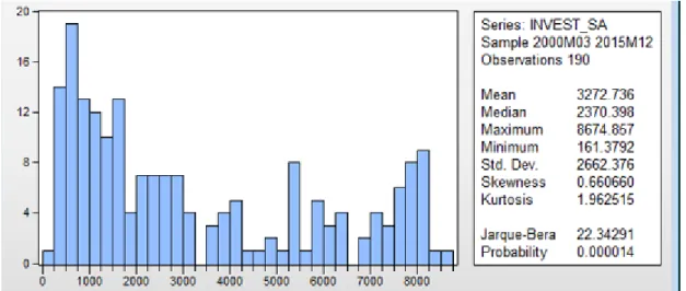
22 Figure 3. Descriptive statistics of Invest-sa
Figure 3 illustrates the basic descriptive statistics of Invest-sa time series. We observe moderate positive skewness and a platykurtic distribution since the kurtosis is lower than 3. The Jarque-Bera test shows that the Invest-sa time series is not normally distributed since the probability value is less than 0.05 (that is, the 5% significance level). By observing the graph (from Figure 1), we can find a linear trend, the mean is larger than 0, so we can conclude that there is also an intercept.
Figure 4. Descriptive statistics of the M2 variable
Figure 4 illustrates the basic descriptive statistics of the M2 time series. We observe some moderate positive skewness and a platykurtic distribution since the kurtosis is lower than 3. The Jarque-Bera test shows that the time series is not normally distributed since the probability value is less than 0.05 (that is, the 5% significance level). We also can observe a linear trend and a non-zero intercept.
23 Figure 5. Descriptive statistics of the MB
Figure 5 illustrates the basic descriptive statistics of the MB time series, where we observe once again moderate positive skewness and a platykurtic distribution since the kurtosis is lower than 3. The Jarque-Bera test shows that the time series is not normally distributed since the probability value is less than 0.05(that is, the 5% significance level). From the graph, we can find a linear trend and a non-zero intercept.
Figure 6. Descriptive statistics of Stock Market
Figure 6 illustrates the basic descriptive statistics of Stock Market time series, where we observe positive skewness and a leptokurtic distribution since the kurtosis is higher than 3. The Jarque-Bera test shows that the time series is not normally distributed since the probability value is less than 0.05 (that is, the 5% significance level). From the graph, we cannot find any monotone trend, but since the mean is larger than 0, so
24 we can conclude that there is a non-zero intercept.
Table 1 summarize the conclusion we can get from the descriptive statistic of each one of the variables:
Intercept Trend Seasonality Outlier Normally
distributed
CPI Yes No No Yes No
Investment Yes Yes Yes No No
Investment-sa Yes Yes No Yes No
MB Yes Yes No No No
M2 Yes Yes No No No
Stock Market Yes No No Yes No
Table 1. Conclusion of descriptive statistics for all selected variables
3.2.2 Unit root test and VAR model
We say that a time series, {𝑦𝑡}, t = 1,…,T, is weak stationary if the mean and the variance are constant on time and the covariance only depends on the lag and does not depends on time, that is:
(1)
E
y
t
,
t
,(2)
var
y
t
2
,
t
(3)cov
y
t,
y
tk
k,
t
Where 𝜇 is the mean, 𝜎2 is the variance and 𝛾
𝑘 is the covariance of the random
variable 𝑦𝑡.
In order to test if the time series are stationary, we used three specific tests, namely Augmented Dickey-Fuller (ADF test), Kwiatkowski–Phillips–Schmidt–Shin (KPSS) and the Phillips-Perron (PP) test. These tests differ in how they treat serial correlation in the test regressions. ADF test use a parametric autoregressive structure to capture
25 serial correlation and PP tests use non-parametric corrections based on estimates of the long-run variance of ∆𝑦𝑡, where ∆𝑦𝑡 denotes the first order difference of the time series 𝑦𝑡.
For the ADF and PP test the null hypothesis is:
H0: there is an unit root (the time series is non-stationary) VS
H1: there is no unit root for the time series (the time series is stationary).
For the KPSS test, the null hypothesis is: H0: the time series is stationary VS
H1: the time series is non-stationary.
Table 2 presents the output conclusions of the ADF, KPSS and PP test employed to each one of the time series in levels.
ADF PP KPSS
t-value Prob t-value Prob 5% critical value KPSS statistic CPI -2.60 0.939 -2.79 0.0611 0.463 0.313 Invest SA -1.97 0.613 -2.38 0.389 0.146 0.402 M2 -0.65 0.97 -0.62 0.98 0.146 0.428 MB -2.34 0.407 -2.03 0.583 0.146 0.388 Stock Market -2.37 0.150 -2.24 0.194 0.463 0.543
Table 2⑧. Unit root tests conclusions for time series in levels
From this table we can infer that none of these time series are stationary in level, since the p-value is higher than 5% significance level and we do not reject the null (ADF, PP), so we proceed to stationarize the data by using the first-order difference operator.
26 In what follows we apply the considered unit root tests on the first difference of these variables and we conclude about stationarity in Table 3:
ADF PP KPSS
t-value Prob t-value Prob 5% critical
value KPSS statistic △CPI -6.06 0 -13.31 0 0.463 0.05 △Invest SA -15.5 0 -26.28 0 0.146 0.120 △M2 -2.98 0.141 -14.89 0 0.146 0.069 △MB 0.119 0.997 -15.38 0 0.146 0.20 △Stock Market -7.23 0 -12.75 0 0.146 0.040
Table 3⑨. Unit root tests for the first order differenced time series
According to the result of PP test, we found that, all these 5 variables are stationary in first difference since we reject the null. Further, we can see that, when we take unit root test of M2 and MB in first differences, they don’t pass the ADF and KPSS test except M2, that pass KPSS, being stationary (the KPSS statistics it is higher than the 5% critical value). This is no problem, because usually, economic time series are stationary in same rank. Further, we employ unit root test on M2 and MB in second difference just to see what would happen, and the result is that they passed all 3 tests, but we cannot understand why “the change of change amount of M2/MB is related with the change of the remaining variables”, it seems meaningless. On the other hand, all the time series passed the PP test in the first difference, and since this is the most credible and powerful one between the 3 unit tests, we can conclude that the five considered time series are integrated of order 1, that is, I(1).
In what follows we are going to use the first difference of these 5 variables in order to build a VAR model adequate to analyze the relation between these variables. We study several variable combinations in the VAR models and reject some of them based
27 on the residuals properties. Since M2 and MB’s impacts in the VAR model are coincidental, we only put one of them into the model each time. The following table makes the summary of some VAR models based on the lag structure (Information Criteria based) and the residual correlation (Portmanteau Test):
VAR with M2 VAR with MB
Suggested lags If residuals correlated
Suggested lags If residuals correlated 3 yes 1 yes 6 yes 2 no 10 yes 3 yes 12 yes 20 yes 24 yes
Table 4⑩. Lag number and residual correlation in considered VAR models
We can conclude from Table 4 that the VAR model that includes the variables CPI, MB, Invest SA and Stock Market in first differences with 2 lags is the only model with uncorrelated residuals. For this reason this will be the model we consider further in our analysis. We also take a look at the AR roots graph, all the points fall in the unit circle, which means the model is stable.
28 Figure 7. The AR roots graph
But usually, we need to take the logarithms (logs) of the variables Invest-sa, MB and Stock Market, this is because CPI is a kind of rate of change, and the other three variables are all real numbers. The huge differences in absolute values between variables in the model may produce too large coefficient of CPI when use the other three variable as dependent variable and too small coefficients of the other three variables when use CPI as the dependent variable. So we take logs of all the variables except CPI (it is already rate of change) to transform them into growth rate.
Theoretically, if the original variables passed the unit root tests, the log of them should also pass the same tests, but for prudency we take all necessary tests to the new generated 3 variables. Because CPI is stationary in first difference, we just test stationarity for the first difference of the newly generated log-variables:
29
ADF PP KPSS
t-value Prob t-value Prob 5% critical value KPSS statistic ΔLogInvestSA -9.02 0.00 -64.37 0.00 0.146 0.160 ΔLogMB -1.41 0.86 -14.50 0.00 0.146 0.214 ΔLogStock Market -7.53 0.00 -12.47 0.00 0.463 0.572
Table 5⑪. Unit root tests for the growth rate of the considered variables
From Table 5 we can conclude that all three variables are stationary in the first difference of the log of variables as we expected, since based on the PP unit root test we always reject the null of non-stationarity and based on KPSS test we never reject the null of stationarity.
Considering now these variables we test new VAR models and we conclude that for our purpose, the new VAR model best fitting the variables needs 4 lags according to Portmanteau tests⑫ for residual correlation whose null hypothesis is:
H0: no residual autocorrelations up to lag h VS
H1: exists residual autocorrelations up to lag h
Then we have a look at the AR roots graph, all the points fall in the unit circle, which means the model is stable.
⑪ Figure 42-50 in appendix ⑫ Figure 51 in appendix
30 Figure 8. The AR roots graph
As we have explained above, the VAR model is a system of equations designed to analyze how the past (lagged) values of all variables can influence the current value of each variable. So, in our case, we finally got four equations: with ∆𝐶𝑃𝐼, ∆𝐿𝑂𝐺𝑀𝐵, ∆𝐿𝑂𝐺𝐼𝑁𝑉𝐸𝑆𝑇𝐴𝑆𝐴 and ∆𝐿𝑂𝐺𝑆𝑇𝑂𝐶𝐾 as dependent variable in turn and all four period lagged variables in the right-hand side. But according to the main purpose of this thesis, we only want to see how shocks in other variables can make the PBC decide to print money, that is, how shocks in other variables can influence CPI, so we only show up the estimated equation with ΔCPI as dependent variable here, that is:
∆𝐶𝑃𝐼𝑡= 0.03∆𝐶𝑃𝐼𝑡−1+ 0.11∆𝐶𝑃𝐼𝑡−2+ 0.11∆𝐶𝑃𝐼𝑡−3+ 0.07∆𝐶𝑃𝐼𝑡−4− 1.27∆𝐿𝑂𝐺𝑀𝐵𝑡−1+ 0.30∆𝐿𝑂𝐺𝑀𝐵𝑡−2+ 0.08𝐿𝑂𝐺𝑀𝐵𝑡−3− 0.59∆𝐿𝑂𝐺𝑀𝐵𝑡−4+
0.06∆𝐿𝑂𝐺𝐼𝑁𝑉𝐸𝑆𝑇𝐴𝑆𝐴𝑡−1+ 0.80∆𝐿𝑂𝐺𝐼𝑁𝑉𝐸𝑆𝑇𝐴𝑆𝐴𝑡−2+
0.49∆𝐿𝑂𝐺𝐼𝑁𝑉𝐸𝑆𝑇𝐴𝑆𝐴𝑡−3− 0.03∆𝐿𝑂𝐺𝐼𝑁𝑉𝐸𝑆𝑇𝐴𝑆𝐴𝑡−4+ 1.25∆𝐿𝑂𝐺𝑆𝑇𝑂𝐶𝐾𝑡−1−
31
3.2.3 Impulse Response Function
Since VAR model is a kind of non-theoretical model, we need to analyze the impulse response functions (IRF) to see how a shock in residuals (innovations) of each equation in the VAR system would influence on all endogenous variables. Normally we introduce one period standard deviation shock to one of the endogenous variable and we assume that the model is in a stable equilibrium and errors are not correlated.
So the last step is to see the impulse response of 𝐶𝑃𝐼 and 𝑀𝐵 to shocks on different explanatory variables, which can help us answer the questions which are put forward at the beginning of this thesis.
First we take a look at the shape of IRFs.
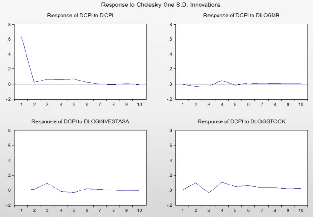
Figure 9 to Figure 12 are the responses of all the four variables to unit shock on all four variables themselves. Among all the impulse response functions, we are most interested in the responses of ∆𝐶𝑃𝐼 to unit shocks of other three variables (we can find the variable that influences inflation most), and the responses of ∆𝐿𝑂𝐺𝑀𝐵 to shocks (which can tell us what kind of volatility can force PBC to print money).
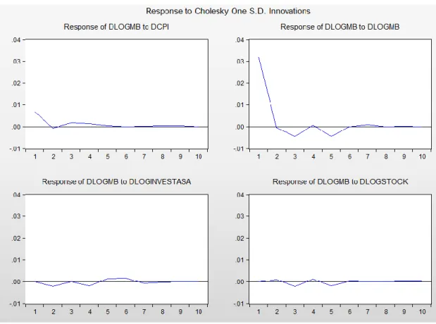
32 Figure 10. Responses of ∆𝐿𝑂𝐺𝑀𝐵 to unit shocks in all four variables
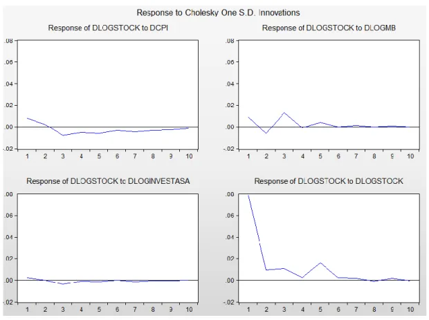
33 Figure 12. Responses of ∆𝐿𝑂𝐺𝑆𝑇𝑂𝐶𝐾 to unit shocks on all four variables
Figure 13. Response of ∆𝐶𝑃𝐼 to a positive shock on ∆𝐿𝑂𝐺𝑀𝐵
From Figure 13 we can infer that when there is a positive shock on ∆𝐿𝑂𝐺𝑀𝐵, the ∆𝐶𝑃𝐼’s reaction is very weak in first 2.5 periods, then it will begin to rise slowly in the middle of 3rd period, after reaching the apex in 4th period it begins to fall and changes the direction of shock impact and become more and more stable, in long run,
34 the shock impact tends to zero.
Figure 14. Response of ∆𝐶𝑃𝐼 to a positive shock on ∆𝐿𝑂𝐺𝐼𝑁𝑉𝐸𝑆𝑇𝐴𝑆𝐴
From Figure 14 we can infer that when there is a positive shock on ∆𝐿𝑂𝐺𝐼𝑁𝑉𝐸𝑆𝑇𝐴𝑆𝐴, the ΔCPI’s begins to rise in the second period and reaches its apex in the 3rd period, after then it begins to fall and changes the direction in middle of the 4th period. In long run, the shock impact tends 0.
Figure 15. Response of ∆𝐶𝑃𝐼 to a positive shock on ∆𝐿𝑂𝐺𝑆𝑇𝑂𝐶𝐾
35 From Figure 15 we can infer that when there is a positive shock on ∆𝐿𝑂𝐺𝑆𝑇𝑂𝐶𝐾, the ∆𝐶𝑃𝐼 will begin to rise immediately and reaches its apex in the middle of 2nd period,
after then it decreases and changes the direction in middle of 3rd period and changes the direction once again, in 4th period it reaches the apex once again and decreases mildly until the impact of the shock diminishes in long run.
Figure 16. Response of ∆𝐿𝑂𝐺𝑀𝐵 to a positive shock on ∆𝐶𝑃𝐼
36 Figure 18. Response of ∆𝐿𝑂𝐺𝑀𝐵 to a positive shock on ∆𝐿𝑂𝐺𝑆𝑇𝑂𝐶𝐾
From figure 16-18, we can infer that, the ∆𝐿𝑂𝐺𝑀𝐵 reacts weakly to shocks on ∆𝐿𝑂𝐺𝑆𝑇𝑂𝐶𝐾 and ∆𝐿𝑂𝐺𝐼𝑁𝑉𝐸𝑆𝑇𝐴𝑆𝐴 though it shows some mild fluctuations at the beginning of the shock, when the shock comes from ∆𝐶𝑃𝐼, the ∆𝐿𝑂𝐺𝑀𝐵 rises sharply at beginning but soon back to the original level after some mild fluctuations.
The most interesting phenomena we can observe from our model is: the reaction of monetary base to shocks in real estate market is much weaker than the reaction of CPI to the same shock.
Related with the most recent crisis in Chinese stock market, PBC faces a problem: the nominal interest rate of one-year deposit has decreased to 1.5% with CPI of 1.5% at the same time. Economic theories told us that usually even the real interest rate is 0 or negative, the central bank can also reduce nominal interest rate to stimulate the economy if the nominal interest rate is still positive, but the Chinese situation is a little different which makes PBC hesitated when decides if reduce the real interest rate below 0: China has super high gross saving rate (GSR), in 2014 the GSR of China was 49% and the GSR of USA was only 18%⑬ at the same time. So if the real interest rate fall
37 below 0, it will release much more money from the bank system than any other country in the world. If the money released from bank system can flood into the stock market, maybe it can still become an attractive option to PBC. But as we have mentioned above, usually the money will enter the real estate market which is helpless to the current crisis in stock market.
So every time when China faces such economic difficulties and announces its aggressive new policies, we can always hearing some people claiming that “Ah, the Chinese QE is coming!”⑭
But the quantitative easing is still harmful to the economy: if central bank issues large amount of banknotes with such high GSR, it will greatly dilute the wealth of the people which may lead to other serious problems, for example, a run on foreign currency.
By watching at the figures we can get some preliminary conclusions, but if we want
some more accurate results with stronger statistical support, we have to analyze the multipliers.
3.2.4 The multipliers
In this section we will analyze the multipliers associated with inflation in our linear VAR system. In particular, we would like to know what happens to inflation (and here we should recall the reader that our variable is DCPI), when there is one shock to the other three variables, one by one. These other variables are the Monetary Base (DLOGMB), the Residential Investment (DLOGINVEST), and the Stock Market Index (DLOGSTOCK). For this purpose we will take into account the Impulse Response Functions (IRF) associated with each shock. Formally this multiplier (m) can be written down as:
𝑚𝑖(𝑡) =∆𝐷𝐶𝑃𝐼(𝑡)∆𝑖(𝑡) (5)
⑭ For example, the Wall Street
journal-http://www.wsj.com/articles/chinas-central-bank-expands-new-style-easing-1444649102
Or Bloomberg- http://www.bloomberg.com/news/articles/2015-08-09/quantitative-easing-with-chinese-characteristics-takes-shape
38 Where i stands either for Monetary Base, the Residential Investment or the Stock Market, and t as a time quarter index.
In the two following figures we present, firstly, the IRFs from each shock, and secondly the multipliers will be displayed. While a simple visual inspection of the evolution of the multipliers looks a little bit confusing, the sum over the period of nine quarters of each multiplier does not leave much room or doubts, which is presented next:
𝛴𝑡=09 𝑚𝐼𝑁𝑉𝐸𝑆𝑇 = 2.5712 (6)
𝛴𝑡=09 𝑚𝑀𝐵 = 14.5316 (7) 𝛴𝑡=09 𝑚𝑆𝑡𝑜𝑐𝑘 = −2.2956 (8) These cumulative values of the multipliers allow us to conclude that a positive shock to the Stock Market (DLOGSTOCK) will produce a negative impact upon inflation (DCPI) by a degree of -2.2956. On the other hand, an increase in Residential
Investment will lead to a positive impact upon inflation of a magnitude close to 2:5. However, the variable that shows a huge impact upon inflation in this our linear VAR model is the Monetary Base. In our case, if the logarithmic value of the Monetary Base increases by one standard deviation, the change in the CPI will be increased by 14.53 after just nine quarters.
39 Figure 19 The IRFs of inflation associated with each individual shock.
Figure 20 The multipliers
Apparently, these results seem to show some support to the quantity theory of money in China. Real variables, like residential investment show a rather small
0 1 2 3 4 5 6 7 8 9 -0.1 0 0.1 0.2 0.3 0.4 0.5 0.6 0.7
Responses from a shock to Inflation
CPI MB INVEST Stock 0 1 2 3 4 5 6 7 8 9 -0.2 -0.15 -0.1 -0.05 0 0.05 0.1 0.15
Responses from a shock to Residential Investment
CPI MB INVEST Stock 0 1 2 3 4 5 6 7 8 9 -0.005 0 0.005 0.01 0.015 0.02 0.025 0.03 0.035
Responses from a shock to the Monetary Base
CPI MB INVEST Stock 0 1 2 3 4 5 6 7 8 9 -0.01 0 0.01 0.02 0.03 0.04 0.05 0.06 0.07 0.08
Responses from a shock to the Stock Market
CPI MB INVEST Stock 0 1 2 3 4 5 6 7 8 9 -6 -4 -2 0 2 4 6 8 10 12 The multipliers Residential Investment Monetary Base Stock Market
40 positive impact upon inflation, and wealth variables (like the stock market index) do show a rather negative small impact upon such variable. This last result looks interesting, because one would expect capital gains (in the stock market) to be positively correlated with inflation, but that is not the case in our model. This may look the result of a similar situation that we have observed in economies under large QE interventions (as is the US case), where the liquidity trap and deflation redirect investments into the stock market, leading to a situation in which we have deflation and rising stock market indexes.
However, the case of China does not allow us to infer that QE suffers from the same limitations as in the US. If our linear model is consistent and robust enough (we could not afford to go into more sophisticated nonlinear VAR analysis due to time
limitations associated with a thesis of this nature) with the reality in the Chinese economy, there seems to exist plenty of scope to use monetary policy in China in order to avoid deflation and the slowdown of the Chinese economy, because the monetary base multiplier shows a remarkable cumulative value of 14.5 in just 9 quarters. Therefore, and in the period considered in this study, the limitations of QE as we start to feel in the western economies and Japan, do not apparently apply to the Chinese economy.
41
4. Concluding Remarks
So let us answer the three questions at the beginning of this thesis.
1. Are the policies pursued by PBC QE? Theoretically, the answer is “No”. We know that the central bank threaten to abandon conventional monetary policy to adjust the economy, in practice they even printed some money but behaved extremely restraint to reduce the negative effect as much as possible. So it seems that PBC prefers Krugman’s suggestion in theory but Japan’s strategy in practice: printing money may acceptable, but the final goal is to produce inflationary expectation of the market, so if possible, the less additional money the better. When a central bank is losing its credit, it has to behave as mad as possible to convince the public again, but the situation of PBC seems better, so even it didn’t have much space to reduce the nominal interest rate, it can still produce inflationary expectation by printing less money than western countries. If the conventional monetary policy is still in effect, why should we use QE?
2. Did they achieve the goal of alleviating the crisis? Yes, after announcing the aggressive economic policy, the stock market stopped its sharp fall in a week. 3. In which situation PBC will consider using real QE? Because deflation and the
stringent limitations of monetary policy in the Zero Lower Bound do not seem to be applying to the Chinese economy by now, as well as the near future is concerned. At least we can say, in the near future within two years (we just calculated nine quarters’ accumulative multipliers, so we can just predict the situation of next two years), and PBC doesn’t have the motivation to apply QE policy when the conventional monetary policy is still strong enough to control the economy.
So, here we can conclude the behavior pattern of PBC: when there is a shock-could be in any important economic area, it tends to threaten the market by announcing very aggressive attitude, for example, a large scale QE (they never call it QE, even all economists suspect it is QE in fact, this is a kind of fuzz strategy to stimulate the economy while keeping the confidence of market at the same time) to show its steady will to stabilize the market, but act as conservative as possible in real operation. Until
42 now, we can’t see any sign of the arrival of Chinese QE policy, at least in the near future, China can still act as one of the main growth point of global economy even it faces risks in some important areas.
43
5. Appendix
Figure 1 ADF test result of CPI in level
Figure 2 PP test result of CPI in level
Figure 3 KPSS test result of CPI in level
44 Figure 5 PP test result of INVEST-SA in level
Figure 6 KPSS test result of INVEST-SA in level
Figure 7 ADF test result of M2 in level
45 Figure 9 KPSS test result of M2 in level
Figure 10 ADF test result of MB in level
Figure 11 PP test result of MB in level
46 Figure 13 ADF test result of STOCK MARKET in level
Figure 14 PP test result of STOCK MARKET in level
Figure 15 KPSS test result of STOCK MARKET in level
47 Figure 17 PP test result of CPI in first order difference
Figure 18 KPSS test result of CPI in first order difference
Figure 19 ADF test result of INVEST-SA in first order difference
48 Figure 21 KPSS test result of INVEST-SA in first order difference
Figure 22 ADF test result of M2 in first order difference
Figure 23 PP test result of M2 in first order difference
49 Figure 25 ADF test result of MB in first order difference
Figure 26 PP test result of MB in first order difference
Figure 27 KPSS test result of MB in first order difference
50 Figure 29 PP test result of STOCK MARKET in first order difference
Figure 30 KPSS test result of STOCK MARKET in first order difference
Figure 31 Lag length analysis of VAR model with first order differences of CPI, M2, INVEST-SA and STOCK MARKET under different criterias