A comparative study of the dynamic critical behavior of the four-state Potts like models

Contents lists available atScienceDirect

Physica A

journal homepage:www.elsevier.com/locate/physa

A comparative study of the dynamic critical behavior of the four-state

Potts like models

E. Arashiro

a,∗

, H.A. Fernandes

b

, J.R. Drugowich de Felício

c

a_{Universidade Federal de Ouro Preto, Departamento de Física, Campus Universitário Morro do Cruzeiro, Ouro Preto, MG, 35400-000, Brazil} b_{Universidade Federal de Goiás, Campus Jataí, BR 364, Km 192, n. 3800, C.P. 03, Setor Parque Industrial, Jataí, GO, 78000-000, Brazil}

c_{Universidade de São Paulo, Faculdade de Filosofia, Ciências e Letras de Ribeirão Preto, Avenida Bandeirantes, n. 3900, Ribeirão Preto, SP, 14040-901, Brazil}

a r t i c l e i n f o

Article history: Received 26 March 2009

Received in revised form 16 June 2009 Available online 10 July 2009 PACS:

64.60.Ht 75.10.Hk 02.70.Uu Keywords:

Monte Carlo simulations Dynamic critical exponents Out-of-equilibrium systems Non-Markovian process Universality class

a b s t r a c t

We investigate the short-time critical dynamics of the Baxter–Wu (BW) andn₌3 Turban (3TU) models to estimate their global persistence exponentθg. We conclude that this new

dynamical exponent can be useful in detecting differences between the critical behavior of these models which are very difficult to obtain in usual simulations. In addition, we estimate again the dynamical exponents of the four-state Potts (FSP) model in order to compare them with results previously obtained for the BW and 3TU models and to decide between two sets of estimates presented in the current literature. We also revisit the short-time dynamics of the 3TU model in order to check if, as already found for the FSP model, the anomalous dimension of the initial magnetizationx0could be equal to zero.

©2009 Elsevier B.V. All rights reserved.

1. Introduction

Since the works by Janssen, Schaub and Schmittmann [1], and Huse [2], the critical properties of statistical systems have been a subject of considerable interest in non-equilibrium physics [3–13]. By using renormalization group methods and numerical calculations, respectively, they showed that there is universality and scaling behavior even at the early stage of the time evolution after quenching from high temperatures to the critical one.

The dynamic scaling relation obtained by Janssen et al. [1] for thekth moment of the magnetization, extended to systems of finite size [3], is written as

M(k)

(

t

, τ ,

L

,

m0

)

=

b−kβ/νM(k)

(

b−zt

,

b1/ν

τ ,

b−1L

,

bx0_m0

_),

₍₁₎ wheretis the time evolution,bis an arbitrary spatial scaling factor,

τ

=

(

T

−

Tc

)/

Tcis the reduced temperature andLis the

linear size of the lattice. The exponents

β

and

ν

are as usual the equilibrium critical exponents associated respectively with the order parameter and the correlation length,zis the dynamical exponent characterizing time correlations in equilibrium, andx0represents the anomalous dimension of the initial magnetizationm0, introduced to describe the dependence of the scaling behavior on the initial conditions.

Besides to avoid the well-known problem of the ‘‘critical slowing down’’, characteristic of the equilibrium, and to provide an alternative way to obtain the familiar set of static critical exponents and the dynamic critical exponentz, this kind of investigation reveals a new universal regime and an unsuspected new dynamic critical exponent

θ

which can be found by

∗Corresponding author. Tel.: +55 313559 1678; fax: +55 31 3559 1667. E-mail address:[email protected](E. Arashiro).

following the above scaling law for the order parameter at the critical temperature (τ

=

0)

M

(

t

)

∼m0tθ

.

(2)

This new index, independent of the previously known exponents characterizes the so-called ‘‘critical initial slip’’, the anomalous behavior of the order parameter when a system is quenched to the critical temperatureTc. This exponent is

related tox0as

θ

=

x0

−

β/ν

z

.

(3)

Some years later, Majumdar et al. [14] have shown that another dynamic critical exponent can be obtained in the study of systems far from equilibrium. By studying the behavior of the global persistence probabilityP

(

t

)

that the order parameter has not changed its sign up to timet, they have shown thatP

(

t

)

should behave, at the critical temperature, as

P

(

t

)

∼t−θg

,

(4)

where

θ

gis the global persistence exponent. They also argued that, if the time evolution of the order parameter would be a

Markovian process, then the exponent

θ

gshould obey the equation [14]

θ

g

=

α

g

= −

θ

+

d 2z

−

β

ν

z

.

(5)

However, as shown in several works [14–26] the exponent

θ

g is an independent critical index closely related to the

non-Markovian characteristic of the process.

In this work, we perform short-time Monte Carlo simulations to investigate the scaling behavior of the global persistence probabilityP

(

t

)

for the BW [27,28], 3TU [29,30] and FSP [31,32] models in two dimensions (d

=

2), that exhibit the same set of leading static critical exponents. We also calculate the exponentx0of these models but only after reobtaining more precise estimates for the dynamical indices

θ

andzrelated to the FSP and 3TU models. The aim of this paper is to show that it is also possible to detect different behavior between those models by doing short-time Monte Carlo simulations.

The paper is organized as follows. In the next section we present the models. In Section3we show the short-time scaling relations and present our results. Finally, in Section4we present our conclusions.

2. The models

Theq-state Potts model which is a simple extension of the Ising model, has a rich phase diagram [32] with first order phase transitions whenq

>

4 and second order phase transitions whenq

≤

4. Its Hamiltonian is given by

−

β

H

₌

K

X

hi,ji

δ

σiσj

,

(6)

where

β

=

1/kBT and kB is the Boltzmann constant,

h

i

,

j

i

represents nearest-neighbor pairs of lattice sites, K is the

dimensionless ferromagnetic coupling constant and

σ

iis the spin variable which takes the values

σ

i

=

0, . . . ,q

−

1 on

the lattice sitei. It is well known that the critical coupling of this model is given by Ref. [32]

Kc

=

log(1

+

√

q

),

(7)

and its order parameter is defined as

M

=

1

Ld

₍

_q

₋

₁₎

*

X

i

(

q

δ

σi(t),1

−

1)

+

(8)

whereLis the linear size of the lattice anddis the dimension of the system. The caseq

₌

4 (FSP model) in two dimensions is known to exhibit slow convergence when investigated by finite-size techniques motivated by the presence of a marginal operator (scaling dimension

=

d

=

2).

The BW model is defined by the Hamiltonian

−

β

H

₌

_K

X

hi,j,ki

σ

i

σ

j

σ

k

,

(9)

where

σ

i

= ±

1 is an Ising spin variable located at each site of the triangular lattice and the sum extends over all elementary

triangles.

The Hamiltonian of the 3TU model is given by

−

β

H

₌

X

hi,ji

Kh

σ

i,j

σ

i₊1,j

σ

i₊2,j

+

Kv

σ

i,j

σ

i,j₊1

,

(10)

where the sum is over all sites of a square lattice,KhandKvare the coupling constant in the horizontal (with three-spin interactions) and vertical (with two-spin interactions) directions, respectively, and

σ

i,j

= ±

1 is an Ising spin variable located

at each site of the lattice.

temperatureKc

=

0.5 ln(1

+

√

2)which is the same critical temperature of the Ising model on a square lattice. The order parameter of these models is defined as

M

=

1

Ld

*

X

i

σ

i

+

.

(11)

The BW and 3TU models present semi-global up-down spin reversal symmetry [33], i.e., their Hamiltonians are invariant under reversal of all the spins belonging to two of three sublattices into which the original lattice can be decomposed.

The ground state of these three models is fourfold degenerated, being that the possible spin configurations of the BW and 3TU models consist of repetitions of the patterns

_{+

,

+

,

+}

,

_{+

,

−

,

−}

,

_{−

,

+

,

−}

or

_{−

,

−

,

+}

. The main difference between the three models is that the BW model is defined on a triangular lattice whereas in the FSP and 3TU models the spins are located on a square one.

From the degeneracy and symmetry considerations, it was conjectured that these three models would belong to the same universality class, with critical exponents given by Ref. [34]

β

=

1

12

,

ν

=

α

=

2

3

,

and

η

=

1

4

.

(12)

However, when these models are deeply studied, differences among sub-dominant exponents appear. These exponents are supposed to be associated to different behavior exhibited by those models when studied by finite-size scaling techniques. This fact was first pointed out by Alcaraz and Xavier [35] in a finite-size scaling study of the FSP and BW models using a conformal invariance approach.

As will be shown in this paper, it is possible to observe remarkable differences between those models by investigating the non-equilibrium evolution of a dynamical quantity introduced by Majumdar et al. [14], the global persistence probability. This result corroborates previous simulations which pointed out different behavior for the BW model when compared to the FSP model [36–38].

3. Results and discussions

In our Monte Carlo simulations, we consider two-dimensional lattices with periodic boundary conditions. The dynamical evolution of the spins is local and updated by the heat-bath algorithm at the critical couplingKc. In order to check finite-size

effects, we consider three different lattice sizes (L

=

120, 180 and 240) the exponents being obtained from five independent bins of 20 000 samples each one.

3.1. Global persistence exponent

θ

g

The global persistence probabilityP

(

t

)

can be defined as

P

(

t

)

=

1

−

t

X

t′₌1

ρ(

t′

)

(13)

where

ρ(

t′

₎

_{is the fraction of the samples that have changed their state for the first time at the instantt}′_{. The dynamical} exponent

θ

gthat governs the behavior ofP

(

t

)

at criticality is obtained through the power law behavior given by

P

(

t

)

∼t−θg

.

(14)

In order to obtain the exponent

θ

g, the initial configuration of the system should be carefully prepared with a precise and

small value ofm0. After estimating

θ

g for a number ofm0values, its final value is obtained from the limitm0

→

0. In this

work, we used 4

_×

10−4

_<

_m

0

≤

5

×

10−3.

As we are considering three models and two different order parameters, it is worth to explain how to obtainm0in each case. At the beginning, each site on the lattice of the FSP model is occupied by a spin variable which takes the values

σ

=

0, 1, 2 or 3 and, for the 3TU and BW models, the sites are occupied by spin variables which take the values

±

1. For each model, the values of spin variables are chosen with equal probability. Afterward, the magnetization of the models is measured by using Eq.(8)for the FSP model or(11)for the 3TU and BW models. In order to obtain a null value of the initial magnetization, some sites of the lattices are randomly chosen and its signs (or values) are changed. Finally, the desired value for the initial magnetization of each model is obtained by changing the sign (or the value) of

δ

sites on the lattice. When using Eq.(8), the initial magnetization is given by

m0

₌

4δ

3L2 (15)

and a value ofm0is obtained choosing

δ

sites occupied by

σ

=

0, 2 or 3 and substituting them by

σ

=

1. For Eq.(11),m0is simply given by

m0

=

δ

L2 (16)

300 50

0.02

0.01

100 t

200

300

50 100

t

200

300

50 100

t

200

P(t)

0.01 0.1

P(t)

0.01

0.001 0.1

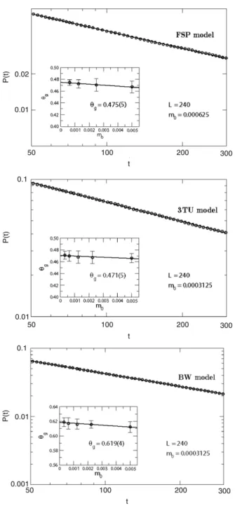
P(t)

Fig. 1. The time evolution of the global persistence probabilityP(t)forL= 240 for the FSP (on top), 3TU (on middle), and BW (on bottom) models. The error bars calculated over 5 sets of 20 000 samples are smaller than the symbols. The inset in each figure shows the exponentθgfor different initial

magnetizations, as well as its extrapolated value.

InFig. 1we show the behavior of the global persistence probability forL

=

240 and a small value ofm0for the FSP (on top), 3TU (on middle), and BW (on bottom) models, in double-log scales. The error bars, calculated over five sets of 20 000 samples are smaller than the symbols.

The insets inFig. 1display the estimates of

θ

g for different values ofm0and the limiting procedurem0

→

0 for the

models.

InTable 1, we show the extrapolated values of

θ

g forL

=

120, 180 and 240 for the BW, 3TU and FSP models. Finite-size

effects are less than statistical errors.

Table 1

The global persistence exponentθgfrom the power law behavior for the FSP, 3TU, and BW models.

Models L₌120 L₌180 L₌240

FSP 0.469(4) 0.472(6) 0.475(5)

3TU 0.469(6) 0.470(5) 0.471(5)

BW 0.620(5) 0.618(5) 0.619(4)

Table 2

The exponentθfor the FSP and 3TU models.

L FSP model 3TU model

120 ₋0.046(8) ₋0.047(7)

180 ₋0.047(8) ₋0.046(7)

240 −0.046(9) −0.047(8)

Table 3

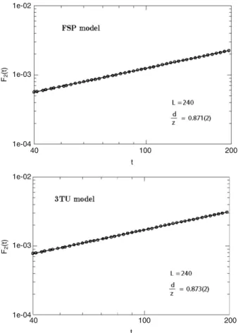
The exponentzfor the FSP and 3TU models.

L FSP model 3TU model

120 2.294(7) 2.293(5)

180 2.294(5) 2.290(8)

240 2.296(5) 2.292(4)

made on finite lattices (at the equilibrium) it is well known that BW, FSP and 3TU models show different corrections to finite-size scaling. Whereas estimates for the BW model exhibit good convergence with the system size [35], comparable to that of the two-dimensional Ising model, FSP and 3TU models offer serious barriers to whom wish to find their exponents from finite-size techniques [39,40].

3.2. Dynamic critical exponents

θ

and z

As conjectured by Janssen et al. [1] on the basis of renormalization group techniques and by Huse [2] through numerical calculations, in the short-time regime, the order parameter obeys a power law as shown in Eq.(2). Formerly, a positive value was always associated to this exponent [5,41–44] and the phenomenon was known as critical initial slip. However, as shown in some papers, there are models in which the exponent

θ

can have a negative value, for instance, the tricritical Ising model, [45,46], FSP [47], 3TU [48], and BW [37,49] models.

Although the estimates of the exponents

θ

andzfor the BW model are known with good precision, the results for the 3TU model exhibit large error bars. In addition, estimates obtained for

θ

in previous papers [25,47] show considerable differences between the two techniques employed to study the FSP model. So, in order to obtain more precise estimates for the exponentx0, we decided to reobtain the exponents

θ

andzfor both FSP and 3TU models by using the time correlation of the magnetization [43]

C

(

t

)

= h

M

(0)

M

(

t

)

i

∼tθ (17)

and the functionF2

(

t

)

proposed by da Silva et al. [9]

F2

(

t

)

=

h

M2

₍

_t

₎

i

m₀₌0

h

M

(

t

)

i

2

m0=1

∼td/z

.

(18)

In Eq.(17), the average is taken over a set of random initial configurations. Initially, this approach had shown to be valid only for models which exhibit up-down symmetry [43]. Nevertheless, it has been later found that this approach is more general and can include models with other symmetries [50]. This method has several advantages when compared to other approaches, for instance, the exponent

θ

can be directly calculated without the need of careful preparation of the initial states nor of the limiting procedure [see Eq.(2)], the only requirement being that

_h

M

(0)

_{i =}

0.

InFig. 2we show the evolution of the time correlationC

(

t

)

in double-log scale for the FSP (on top) and 3TU (on bottom) models, respectively, forL

=

240.

The slope of these curves is shown inTable 2, as well as the estimates forL

₌

120, 180 and 240.

On the other hand, the dynamical exponentzwas obtained by combining results from samples submitted to different initial conditions (see Eq.(18), whered

₌

2 is the dimension of the system). This approach has proved to be very efficient in estimating the exponentzfor several models [9,46,37,44]. The time evolution ofF2is shown on log scales inFig. 3for L

=

240 for the FSP (on top) and 3TU (on bottom) models.

Taking into account the values of the ratiod

/

z, estimated from the slope of these curves, the exponentzcan be easily found. Our estimates for this exponent for the FSP and 3TU models are shown inTable 3forL

=

120, 180, and 240.

C(t)

50 1e-05

5e-06

2e-06

1e-05 1e-04 10

t

100

100

C(t)

1e-06 2e-04

20

t

200

Fig. 2. The time correlation of the order parameter on log scales for the FSP (on top) and 3TU (on bottom) models. Error bars were calculated over 5 sets of 20 000 samples.

Table 4

The exponentαgfor the FSP, 3TU, BW models.

Models αg

FSP 0.427(10)

3TU 0.429(9)

BW [37] 0.567(3)

FSP and 3TU models (Table 2) are completely different from the previously estimated exponent for the BW model [37]

θ

= −

0.186(2). (19)

3.3. The exponent

α

gand the anomalous dimension x0

Using the results ofTables 2and3forL

=

240 (FSP and 3TU models), the results of Eq.(19)and the values of

β

and

ν

of Eq.(12)we estimate the exponent

α

g through Eq.(5)for the studied models (seeTable 4). The difference between our

estimate for

θ

g(SeeTable 1) and the value obtained from Eq.(5)shows the non-Markovian aspect for the BW, 3TU and FSP

models. Thus, the global persistence exponent in these cases is also independent of other critical exponents.

We remark that using the estimates of Hadjiagapiou et al. [49] for the dynamical exponents of the BW modelz

=

1.994(24)and

θ

= −

0.185(2)we obtain

α

g

=

0.624(3)approximately equal to

θ

g (fromTable 1) which means that

the relaxation would be Markovian. As we know, the models studied until now [14–26] exhibit different values for those exponents and this would be the first case where Eq.(5)would be valid.

Finally, we calculate the value of the anomalous dimensionx0of the order parameter for the FSP, 3TU, and BW models. This exponent, which is introduced to describe the dependence on the scaling behavior of the initial conditions, is related to the exponents

θ,

z, and

β/ν

by Eq.(3). So,

x0

₌

θ

z

₊

β/ν.

(20)

40 1e-03

1e-02

1e-03

1e-04

100 t

200

40 100

t

200 1e-02

1e-04 F2

(t)

F2

(t)

Fig. 3. The time evolution ofF2(t)forL=240 for the FSP (on top) and 3TU (on bottom) models. Each point represents an average over 5 sets of 20 000

samples and the error bars are obtained of them. Table 5

The exponentx0for the FSP, 3TU, BW models.

Models x0

FSP 0.019(21)

3TU 0.017(18)

BW [37] −0.302(6)

BW [49] −0.244(8)

As we can see inTable 5, our results indicate that far from equilibrium the critical behavior of the FSP and 3TU models is very similar but different from the BW one. In addition, our estimates do not exclude a null value for the anomalous dimension of the magnetization (x0) in those cases (FSP and 3TU models) which in static critical phenomena theory is known to be associated to marginal operators [51] and in finite-size scaling calculations to logarithmic corrections [52,53].

4. Conclusions

We estimated the dynamical exponent

θ

g for the BW, 3TU, and FSP models using the time evolution of the global

persistence probability that the magnetization has not changed its signal up to timet. The value of

θ

g found for the BW

Acknowledgments

This work was supported by the Brazilian agencies CAPES, CNPq and FAPESP. One of us (H.A.F.) would like to thank the Universidade Federal de Goiás (PRPPG and FUNAPE).

References

[1] H.K. Janssen, B. Schaub, B. Schmittmann, Z. Phys. 73 (1989) 539. [2] D.A. Huse, Phys. Rev. B 40 (1989) 304.

[3] Z.B. Li, L. Schulke, B. Zheng, Phys. Rev. Lett. 74 (1995) 3396.

[4] T. Tome, J.R. Drugowich de Felício, Modern Phys. Lett. B 12 (1998) 873. [5] B. Zheng, Internat. J. Modern. Phys. B 12 (1998) 1419.

[6] B.C.S. Grandi, W. Figueiredo, Phys. Rev. E 70 (2004) 056109.

[7] E. Arashiro, J.R. Drugowich de Felício, U.H.E. Hansmann, Phys. Rev. E 73 (2006) 040902; J. Chem. Phys. 126 (2007) 045107. [8] X.W. Lei, B. Zheng, Phys. Rev. E 75 (2007) 040104.

[9] R. da Silva, N.A. Alves, J.R. Drugowich de Felício, Phys. Lett. A 298 (2002) 325. [10] A. Asad, B. Zheng, J. Phys. A: Math. Theor. 40 (2007) 9957.

[11] L. Környei, M. Pleimling, F. Igloi, Phys. Rev. E 77 (2008) 011127.

[12] S.D. da Cunha, U.L. Fulco, L.R. da Silva, F.D. Nobre, Eur. Phys. J. B 63 (2008) 93. [13] K. Nam, B. Kim, S.J. Lee, Phys. Rev. E 77 (2008) 056104.

[14] S.N. Majumdar, A.J. Bray, S.J. Cornell, C. Sire, Phys. Rev. Lett. 77 (1996) 3704. [15] S.N. Majumdar, A.J. Bray, Phys. Rev. Lett. 91 (2003) 030602.

[16] L. Schulke, B. Zheng, Phys. Lett. A 233 (1997) 93.

[17] K. Oerding, S.J. Cornell, A.J. Bray, Phys. Rev. E 56 (1997) R25. [18] F. Ren, B. Zheng, Phys. Lett. A 313 (2003) 312.

[19] E.V. Albano, M.A. Muñoz, Phys. Rev. E 63 (2001) 031104. [20] M. Saharay, P. Sen, Physica A 318 (2003) 243.

[21] H. Hinrichsen, H.M. Koduvely, Eur. Phys. J. B 5 (1998) 257. [22] P. Sen, S. Dasgupta, J. Phys. A: Math. Gen. 37 (2004) 11949. [23] B. Zheng, Modern Phys. Lett. B 16 (2002) 775.

[24] H.A. Fernandes, J.R. Drugowich de Felício, Phys. Rev. E 73 (2006) 57101.

[25] H.A. Fernandes, E. Arashiro, J.R. Drugowich de Felício, A.A. Caparica, Physica A 366 (2006) 255. [26] H.A. Fernandes, Roberto da Silva, J.R. Drugowich de Felício, J. Stat. Mech. Theory Exp. (2006) P10002. [27] D.W. Wood, H.P. Griffiths, J. Phys. C 5 (1972) L253.

[28] R.J. Baxter, F.Y. Wu, Phys. Rev. Lett. 31 (1973) 1294. [29] L. Turban, J. Phys. C 15 (1982) L65.

[30] L. Turban, J.M. Debierre, J. Phys. A 16 (1983) 3571. [31] R.B. Potts, Proc. Camb. Phil. Soc. 48 (1952) 106. [32] F.Y. Wu, Rev. Modern Phys. 54 (1992) 235. [33] F.C. Alcaraz, M.N. Barber, J. Phys. A 20 (1987) 179.

[34] R.J. Baxter, Exactly Solved Models in Statistical Mechanics, Academic Press, New York, 1982. [35] F.C. Alcaraz, J.C. Xavier, J. Phys. A 30 (1997) L203.

[36] M. Santos, W. Figueiredo, Phys. Rev. E 63 (2001) 042101.

[37] E. Arashiro, J.R. Drugowich de Felício, Phys. Rev. E 67 (2003) 046123. [38] C. Chatelain, J. Stat. Mech. Theory Exp. (2004) P06006.

[39] F. Iglói, D.V. Kapor, M. Skrinjar, J. Sólyom, J. Phys. A: Math. Gen. 16 (1983) 4067. [40] C. Vanderzande, F. Iglói, J. Phys. A: Math. Gen. 20 (1987) 4539.

[41] A. Jaster, E. Manville, L. Schulke, B. Zheng, J. Phys. A: Math. Gen. 32 (1999) 1395. [42] L. Schulke, B. Zheng, Phys. Lett. A 204 (1995) 295.

[43] T. Tomé, M.J. de Oliveira, Phys. Rev. E 58 (1998) 4242.

[44] H.A. Fernandes, J.R. Drugowich de Felício, A.A. Caparica, Phys. Rev. B. 72 (2005) 054434. [45] H.K. Janssen, K. Oerding, J. Phys. A: Math. Gen. 27 (1994) 715.

[46] R. da Silva, N.A. Alves, J.R. Drugowich de Felício, Phys. Rev. E 66 (2002) 026130. [47] R. da Silva, J.R. Drugowich de Felício, Phys. Lett. A 333 (2004) 277.

[48] C.S. Simões, J.R. Drugowich de Felício, Modern Phys. Lett. B 15 (2001) 487. [49] I.A. Hadjiagapiou, A. Malakis, S.S. Martinos, Physica A 356 (2005) 563. [50] T. Tomé, J. Phys. A: Math. Gen. 36 (2003) 6683.

[51] F.J. Wegner, in: C. Domb, M.S. Green (Eds.), Phase Transitions and Critical Phenomena, vol. 6, Academic Press, New York, 1976. [52] R. Kenna, D.A. Johnston, W. Janke, Phys. Rev. Lett. 96 (2006) 115701.