RBRH, Porto Alegre, v. 23, e54, 2018 Scientific/Technical Article
https://doi.org/10.1590/2318-0331.231820170153
Hydrosedimentological modeling with SWAT using multi-site calibration in nested
basins with reservoirs
Modelagem hidrossedimentológica com o SWAT usando calibração multi-local em bacias embutidas com reservatórios
Paulo Rodrigo Zanin1, Nadia Bernardi Bonuma1 and Claudia Weber Corseuil2
1Universidade Federal de Santa Catarina, Florianópolis, SC, Brasil
2Universidade Federal de Santa Catarina, Araranguá, SC, Brasil
E-mails: [email protected] (PRZ), [email protected] (NBB), [email protected] (CWC)
Received: September 18, 2017 - Revised: August 28, 2018 - Accepted: October 08, 2018
ABSTRACT
Calibration and validation of hydrosedimentological models, usually performed at the outlet of a single basin, does not always correctly represent the hydrosedimentological processes in the different subdivisions of dammed river systems. The aim of this study was to evaluate simple calibration techniques (watershed outlet) and multi-site calibration (watershed outlet and internal reservoirs) with the Soil and Water Assessment Tool - SWAT model, using two nested basins in the southern region of Brazil. Three modeling procedures were analyzed, adjusting the hydrological and sedimentological parameters of the watershed and the reservoirs. It was found that (a) the simplest calibration does not correctly represent the processes in reservoirs; (b) the multi-site calibration provided a better simulation of the hydrosedimentological dynamics of the nested basins; and (c) parameterizations of the SWAT reservoir module have limitations in the context of the study area. The results showed that the multi-site calibration in watershed with reservoirs is more appropriate. Keywords: SWAT model; Multi-site calibration; Reservoirs.
RESUMO
A calibração e validação de modelos hidrossedimentológicos, geralmente realizada na saída de uma única bacia, nem sempre representa
de forma satisfatória os processos hidrossedimentológicos decorrentes nas diferentes subdivisões de sistemas fluviais represados. O objetivo do presente estudo foi avaliar as técnicas de calibração simples (saída da bacia hidrográfica) e multi-local (exutório da bacia hidrográfica e reservatórios internos) do balanço hídrico e sedimentológico em duas bacias embutidas com o modelo Soil and Water Assessment Tool - SWAT. Foram analisados três procedimentos de modelagem, ajustando os parâmetros hidrológicos e sedimentológicos
da bacia hidrográfica e dos reservatórios. Verificou-se que (a) a calibração simples não representou corretamente os processos nos
reservatórios; (b) a calibração multi-local simulou melhor a dinâmica hidrossedimentológica das bacias embutidas; e (c) as parametrizações do módulo de reservatórios do SWAT apresentam limitações no contexto da área de estudo. Os resultados mostraram que a calibração
multi-local em bacias hidrográficas com reservatórios é mais adequada.
INTRODUCTION
Water, the dynamic component of the hydrosedimentological cycle, is part of the weathering and erosion processes of the rocky and pedological substrate, transporting and depositing sediments
through surface runoff and river flow. Therefore, the hydrological
cycle is articulated with other matter and energy cycles, and must be analyzed according to the diversity of its components within the system that integrates them, which will present a unique dynamic because of its spatial/temporal magnitude (KLEMES, 1983;
BLOSCHL; SIVAPALAN, 1995; TUCCI; MENDIONDO, 1997). According to Tucci (2003), the configurations of the hydrological
processes can be classified as 5 magnitudes of spatial scales, which
are: microscale (<10-4 km2), transition γ (10-4 km2 to 10 km2),
mesoscale (10 km2 to 103 km2), transition α (103 km2 to 104 km2)
and macroscale (>104 km2).
In other words, the dominant processes of water flow
and sediment yield are different according to the size of the watershed. Therefore it is necessary to take spatial and temporal criteria into account when choosing the best model to represent the hydrosedimentological phenomenon involved (MERRITT; LETCHER; JAKEMAN, 2003). A model that is often used in several parts of the world (GASSMAN et al., 2007), including Brazil (BRESSIANI et al., 2015), is the Soil and Water Assessment Tool - SWAT (ARNOLD et al., 1998, 2012a). This model was developed by researchers from the Agricultural Research Service of the USA (ARS – USDA) and Texas A&M University. It descends from the Simulator for Water Resources in Rural Basins - SWRRB model (ARNOLD; WILLIAMS, 1987), receiving significant contributions from the Routing Outputs to Outlet - ROTO (ARNOLD; WILLIAMS; MAIDMENT, 1995b) and QUAL2E (BROWN; BARNWELL JUNIOR, 1987) models. The SWAT model is a semi-distributed, watershed scale model based on processes, operating on a daily or sub-daily time scale. Its objective is to evaluate the impact of climate changes, land use/cover and agricultural management on water and sediment balance, nutrients and pesticides for long periods (ARNOLD et al., 2012a).
According to Melo Neto et al. (2014), the SWAT model is
used in watersheds from a micro to a macro scale, and it efficiently
shows the heterogeneity of dominant hydrological processes as a function of the spatial scale. However, the literature showed that the traditional form of calibration in the SWAT model still has limitations for representing the spatial-temporal diversity of the processes in watersheds. Temporally, Muleta (2012) and Zhang et al. (2015a) discuss the limitation of the traditional form of
calibration to represent streamflow in wet and dry periods, proposing
alternative calibrations. Spatially, it was found that while Brighenti, Bonuma and Chaffe (2016) calibrated/validated streamflow in a mesoscale basin, they did not manage to achieve validation at a river gauging station downstream of their basin. Thampi, Raneesh and Surya (2010) and Cho et al. (2013) calibrating/validating
streamflow in basins in the order of transition α and mesoscale,
respectively, managed to validate the simulation in other nested sub-basins on the same scale. Piniewski and Okruszko (2011), in
turn, calibrated/validated the streamflow at 11 different stations of
a macroscale basin. However, when they validated the simulations at 12 sites nested in the different sub-basins calibrated, in areas
of 355 to 1,657 km2, they only had satisfactory results in the
sub-basins greater than 600 km2.
Other studies analyzed the spatial calibrations in nested sub-basins. Melo Neto et al. (2014) achieved a good performance for hydrological calibration/validation in a mesoscale basin, on the contrary of what they obtained for the individual calibration of a nested basin on a microscale. On the other hand, when Aragão et al. (2013) analyzed the transposition of calibrated hydrologic and sedimentological parameters between two mesoscale
nested basins, they found that the process is efficient when the
calibrations made in the smaller basin are transferred to the larger basin, but the same does not occur from the larger basin to the smaller one.
The complexity of transferring information efficiently
between different basin scales may be due to the model structure (SIKORSKA; RENARD, 2017), and/or uncertainties originating in the input and evaluation data (KAVETSKI; KUCZERA; FRANKS, 2006). Another factor is the way in which the calibration of parameters is rendered operational over the watershed (ZEIGER; HUBBART, 2016), since Shen et al. (2013) found that the key parameters of SWAT and their variations are different depending on the type of soil and its use in nested basins.
Studies using the SWAT model, that evaluated the
efficiency of simple calibrations (only at the mouth of a basin) and
multi-site in nested basins (mouths of the main basin and nested sub-basins), such as Qi and Grunwald (2005), Cao et al. (2006), Bekele and Nicklow (2007), Zhang, Srinivasan and Liew (2008), Nairaula et al. (2012), Chiang et al. (2014), Noor et al. (2014), Daggupati et al. (2015), Begou et al. (2016), Zeiger and Hubbart (2016), Shrestha et al. (2016), Eduardo et al. (2016), and Bai, Shen and Yan (2017) achieved a better performance of the model with multi-site calibration, associated with the more realistic representation of the heterogeneity of internal processes of the
watershed. These studies aimed mainly at simulating streamflow (9 studies), secondarily streamflow, sediments and nutrients (3) and finally only streamflow and sediments (1), using 2 to 13 (mean 5)
sub-basins nested in meso to macroscale basins situated in North America (8), Asia (2), South America (1), Africa (1) and Oceania (1). A few studies also evaluated other approaches to calibration (ZHANG; SRINIVASAN; LIEW, 2010; VIGIAK et al., 2015) and analysis of uncertainties (XIE; LIAN, 2013; ZHANG et al., 2015b), associated with the multi-site calibration of nested basins.
Only 4 of the studies on multi-site calibration described above have reservoirs within their drainage area, and only
Vigiak et al. (2015) calibrated their sedimentological parameters without showing details on the hydrological calibration. Considering only simple calibration, many studies with SWAT were performed in basins with the presence of reservoirs, some evaluating the hydrological effect (VAN LIEW; GARBRECHT; ARNOLD, 2003; LINO et al., 2009; WAGNER et al., 2011; ZHANG et al., 2012), sedimentological effect (MISHRA; FROEBRICH; GASSMAN, 2007) and water quality effect (ZHANG et al., 2011) of these
structures. The specific evaluation of the SWAT module of
Vale and Holman (2009) calibrated the level of the Bosherston Lakes in the United Kingdom, that are the mouth of the drainage basin of this lake system due to their function of preventing the continental intrusion of seawater. First, these authors calibrated
the inflow into the lake system and the groundwater level, and
then calibrated the level of the lakes, adjusting the water balance parameters of the drainage basin and of the reservoir module. Wu and Chen (2012) compared 3 water discharge methods from reservoirs in the SWAT model, and only one of them was intrinsic to the model. After calibrating and validating the volume and discharges from the Xinfengjiang reservoir in the south of China, they found that the 3 methods can represent their operational purpose, and that the intrinsic method of SWAT had the worst performance. On the other hand, Kim and Parajuli (2014), after
calibrating and validating the inflows into the flood control reservoir
of Grenada (Mississipi-USA), calibrated and validated the liquid
discharges from this dam and the streamflow from a river gauging
station downstream. This led them to conclude that in dammed river systems it is essential to perform a correct calibration of the reservoir module of SWAT.
Multi-site calibration with reservoirs was applied to macroscale watersheds in Asia (ZHANG et al., 2013) and in Europe (VIGIAK et al., 2017). Zhang et al. (2013) performed multi-site calibration with 20 river gauging stations located immediately downstream from the reservoirs and sluices associated with 19 river gauging stations distant (upstream and downstream) from these water damming structures. The adjusted hydrological parameters refer to the intrinsic processes of the watershed, since they used a new water release method based on the reservoirs and sluices in their study area. These authors obtained satisfactory
simulations at 74% of the 39 stations and concluded that the regulation of river discharges with hydraulic structures strongly affects the results of the SWAT model. Vigiak et al. (2017) did not detail the hydrological procedures in the reservoirs but calibrated sediment deposition at 55 of the 114 reservoirs (many of them nested), using river gauging stations immediately downstream from them. In association with another 214 river gauging stations for calibration and 172 for validation, they obtained satisfactory
simulations, confirming the function of the reservoirs to retain
part of the sediment transported by the rivers.
Aiming to complement the Brazilian and international literature on multi-site and reservoir calibration with the SWAT model, the purpose of the present study was to evaluate simulations with a simple and multi-site calibration of the water and sediment balance, in 2 nested mesoscale basins where there are reservoirs.
The scientific contribution of this study is to verify the efficiency
of the calibration at the mouth of the watershed, to represent the hydrosedimentological balance of reservoirs located in its drainage area, and also the effects of calibrating the reservoirs in the basin that includes them.
MATERIAL AND METHODS
Study area
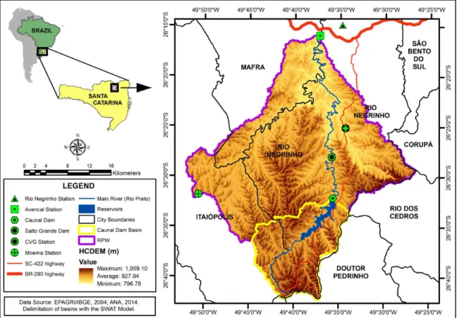
The area studied is the Rio Preto Watershed - RPW, located in the North of the state of Santa Catarina in southern Brazil, as shown in Figure 1. This basin is a sixth order river basin (STRAHLER, 1957), with an area of 965.8 km2 and concentration
time of 18.98h (DOOGE, 1973). The RPW has 2 representative
reservoirs located in one of its 3 fifth order river sub-basins, called
Salto Grande Dam, which belongs to a small hydropower plant and the Caunal Dam which is used to regulate the volume of the Salto Grande Dam (Figure 1). Further details on the contributing basin of the Caunal Dam (199.32 km2), that will be analyzed in
this study can be obtained in Zanin, Bonuma and Franco (2017). The climate in the region, according to the Koeppen
classification, is Cfb, ie., temperate constantly wet without a dry
season and with a cool summer (ALVARES et al., 2013). In the RPW there are sedimentary formations of the volcanic sedimentary basin of Paraná, with porous hydrogeology (CPRM, 2007) and a relief that varies from the steep mountain slopes to gentle hills.
Cambisols (≈85%) and Nitosols (≈12%) predominate in the basin area, with a less significant occurrence of Latosols (≈2%)
and Neosols (< 1%). The RPW is a rural basin with land use and
land cover that are predominantly forests (≈67%), with the rest being used for agriculture and pasture (≈32%), and the presence of water bodies (≈1%).
The RPW was already modeled by Lino et al. (2009) hydrologically using SWAT. However, modelings validating the
streamflow, and also calibration and validation of sediments were
not found for the RPW.
Fluviometric data
In order to evaluate the simple and multi-site calibration
of the SWAT model, the mouth defined for the RPW (Figure 1) was the Avencal river gauging station (Cod. 65094500), which is under the responsibility of the Agência Nacional de Águas - ANA and of the Companhia Paranaense de Energia - COPEL. This station has daily records of water level and point data of liquid discharge, sampled between 1976 and 2015. The point data of Suspended Sediment Concentration - SSC were sampled between 1982 and 2014. Since the Caunal Dam broke in 1983 and was rebuilt in 1985, and the Salto Grande Dam was concluded in 1987,
all the data on level and flow before 1990 were ignored. Due to
the difference in the pattern of the SSC data, before and after the year 2000, the SSC data before this year were also ignored. Since there are gaps in the records of the daily series of levels for
a few short periods at Avencal station, it was necessary to fill out the gaps. It should be pointed out that the only period with filled
out gaps used to evaluate this modeling was the extreme event
that occurred between 7 and 13 June/2014. To fill out the gaps
and also to construct the rating curves simple linear regression
models were used, validated with the coefficient of determination
(R2) (MONTGOMERY; RUNGER, 2003). In order to perform
these parametric analyses, the data were previously transformed with the base 10 logarithm.
In order to fill out the gaps, the data of the river gauging station of Rio Preto do Sul (Cod. 65095000) were used. It lies ≈ 6 km downstream from the Avencal station after the river confluence of Rio Preto with Altíssimo Rio Negro. Data from Rio da Várzea dos Lima river gauging station (Cod. 65135000), located ≈43 km
north from Avencal station were also used, since it is the only station close to the RPW with records of the maximum event
that occurred between 07 and 13 June/2014. Both stations are under the responsibility of ANA/COPEL.
When constructing the regression model between the Avencal and Rio Preto do Sul stations, 4,488 records were used, measured during the period from 01/01/2000 to 06/24/2010.
For the model between Avencal and Rio da Várzea dos Lima stations
the 16 records referring to the recession of the hydrograph of the extreme event of June 2014 were used. The hydrograph recession data were chosen due to the weak determination of the Rio da
Várzea dos Lima station data in relation to the Avencal station
data during the period between 01/01/2000 and 12/31/2014, and the aforementioned extreme rainfall event covered a large space in this region. Thus the behavior of the hydrograph (maximum levels) of these stations originated from the same phenomenon. In order to improve the evaluation of this model, the data simulated and observed for the days from 09/09/2011 to 09/11/2011 were compared. They referred to the peak days of the second largest maximum event that occurred during this modeling period.
The level-flow linear relationship in the RPW was calculated
based on 65 records of liquid discharge measurements associated
with the respective water level. However, analyzing the level-flow
relationship graphically (not shown), it was found that the 3 records were distant from the overall data, and therefore they were eliminated. Moreover, due to the graphic distribution of the data, it was decided to use 2 straight lines of linear adjustment of the
data, having the level of 194 cm (≈ 3° quartile of the sample) as
a threshold, dividing the series into 2 sets of 50 and 12 records. Since one of the straight lines is representative of the 12 highest values sampled, it is then safer to extrapolate the rating curve in relation to the maximum values.
The streamflow-total solid discharge linear relationship
was calculated with 38 records of liquid discharge and SSC measurements. First the suspended solid discharges were calculated using Equation 4.7 of Carvalho et al. (2000), and the bottom solid
discharge using the simplified method of Colby (1957) in WinTSR software (UFSM), obtaining the total solid discharge by adding up
both. Later the regression model between streamflow and total solid discharge was constructed. The streamflow-total solid discharge curve is used due to the absence of linearity between streamflow
and SSC in the RPW, and it is employed in hydrosedimentology studies (CARVALHO et al., 2004; FERNANDES et al., 2005; LOPES et al., 2011).
For the continuous series of liquid and solid discharge from the contributing basin of Caunal Dam (reservoir discharge) daily data were used, calculated from the liquid discharge and 20 point data of suspended solid discharge from the study by Zanin, Bonuma and Franco (2017).
SWAT model
Version 2012 of the SWAT model, revision 627, was used
for hydrosedimentological modeling. The input data required by this model are tabular and spatial information representative of the watershed. The spatial data were interpolated or resampled to a spatial resolution of 10 meters, for the purpose of maintaining the
same resolution to overlay maps in the definition of the Hydrologic
Conditioned Digital Elevation Model (HCDEM); (b) a soil map; and (c) a land use/cover map. Besides the tabular data connected to the maps, SWAT also requires data concerning the characteristics of the channels and dammed water, and also of meteorological variables representing the current climate.
HCDEM
In the HCDEM (Figure 1), altimetric and hydrographic vectorial data were used, mapped to a scale of 1:50,000 (EPAGRI/IBGE, 2004), utilizing Topo to Raster interpolator (HUTCHINSON, 1988; HUTCHINSON, 1989). It should be emphasized that among the cartographic bases available, the one used in this study best represents the dynamic of potential energy of water and of the balance between release and deposition of debris in the RPW (ZANIN; BONUMA; MINELLA, 2017).
Soil map
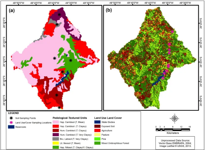
The soil map consisted in editing the base of the Empresa Brasileira de Pesquisa Agropecuária – EMBRAPA (FASOLO et al., 2004), on a scale of detail of 1:250,000. The types of soils in
this base were refined up to the second categorical level of the
new Brazilian soil classification (JACOMINE, 2009), and later by texture. In this way 7 classes of soils were obtained (Figure 2a).
The tabular data on soils associated with the classes of their respective map, were obtained from primary and secondary sources. The depth (SOL_Z) of the deep soil layer was obtained from the cartographic database of EMBRAPA. The hydrologic group (HYDGRP) (USDA, 1972) of each Brazilian soil was
obtained using the classification constructed by Genovez, Lombardi Neto and Sartori (2005). Since SWAT is extremely sensitive to the soil input data (LELIS et al., 2012), a sampling campaign was also performed between 11/04/2014 and 11/08/2014 for the ensemble of soils covered by the basin perimeter, through
Uniform Stratified Random Sampling (BARBETTA, 2011), with a sample of each of the 7 classes of soils, according to Figure 2a.
This sampling campaign aimed at obtaining samples of horizons A and B (except for Neosol, which only has horizon A) to calculate bulk density (SOL_BD), determine the contents of sand (SOL_SAND), silt (SOL_SILT), and clay (SOL_CLAY), organic carbon (SOL_CBN) and organic matter (needed to calculate USLE_K). The saturated hydraulic conductivity data (SOL_K) and the available water capacity of the soil (SOL_AWC) were estimated using ROSETTA software (SCHAAP; LEIJ; VAN GENUCHTEN, 2001) based on grain size and bulk density parameters. Albedo (SOL_ALB) was estimated using the Munsell color table. The depth
of horizon A of each soil was checked in the field.
Figure 2. (a) Soil map and pedological sampling points; (b) Land use/cover map and sampling locations for supervised automatic
Land use/cover map
A 2013 LandSat 8 image (USGS, 2013) was used to elaborate the land use and land cover map (Figure 2b). Based on this image,
and also on verifications in the field between 12/09/2013 and
14/09/2013, homogeneous samples (representative areas) of each
class of use and soil cover were identified. Later, a supervised automatic classification was performed using the non-parametric Parallelepiped method as main classifier, and Maximum Likelihood as secondary classifier. The Kappa index was used to evaluate the accuracy of the classification (CONGALTON; GREEN, 1999).
As regards the tabular data associated with the classes in this map, the information provided was as general as possible for agricultural use, due to the uncertainties about the crops planted and agricultural practices used in the basin studied. Only the value for the factor of conservationist practices of MUSLE (USLE_P) was inferred based on the values tabulated by Wischmeier and Smith (1978), due to the existence of plantations on contour lines, and areas of exposed soil used cyclically for agriculture or reforestation.
As to the tabular data on vegetation, the default values of the SWAT model were used due to the great diversity of species that occur the RPW, with scarce data on their characteristics. Based on the literature on the study area and region, it was possible to insert values for the initial biomass (BIO_INI) (SETTE JUNIOR; GEROMINI; NAKAJIMA, 2004; WATZLAWICK et al., 2012) and maximum storage capacity of water in the tree canopy (CANMX) (CHAFFE, 2009; GIGLIO, 2013), for the Mixed Ombrophile
Forest (FRST) and Pinus (PINE). As the Manning coefficient (OV_N) of the FRST class has a default value (0.1) smaller than
all the other classes of RPW vegetation, its value was made equal to the PINE class (0.14). However, the value of the initial leaf area index (LAI_INI) for the FRST and PINE classes, had its value inferred to 0.5 due to the fact that the default value is zero.
Channel and base flow data
The width of the main channel and the tributaries (CH_W) was adjusted with a multiplicative correction factor (0.31) obtained by the ratio between the mean of the widths measured during the period of this modeling (2009 to 2014) at Avencal station by ANA/COPEL, and the width simulated by SWAT. On the other hand, the simulated depths (CH_D) did not require correction since the depth of the channel at the basin mouth was in accordance with the depth observed at the aforementioned station. Therefore it was necessary to correct the width to depth ratio (CH_WDR).
Since the default value for the Manning coefficient (0.014)
of the main channel and tributaries (CH_N), is smaller than the values tabulated by Chow (1959) for natural channels, this value
was corrected to 0.05 based on field observations performed
during this study, in different sectors of the basin. The values
of the cover factors (CH_COV) of the banks and bed were also
adjusted based on the tabulated values of Julian and Torres (2006). For the bed, which was predominantly soft and without any cover, but with a few hard stretches, the value of the cover factor for the grass-covered bed was used to mitigate the degradation of
the channel in areas with a hard bed, but without significantly
impairing the processes in the soft bed. The value for sparse trees was utilized for the banks.
The median diameter of the sediment (CH_D50) and the bulk density (CH_BD) of the channel banks and bed materials were estimated based on the data sampled from soils, using the mean weighted by the percentage area of each type of soil. The arithmetic mean of horizons A and B of each soil was used to estimate the diameter of the sediment on the banks, while for bed sediments, the value of the banks was used, arbitrarily increased by 50% (D50), and 25% (bulk density), due to the fact that the bed received more deposition of coarse material than the banks (HUDSON-EDWARDS, 2007). To define the D50 based on grain size of horizons A and B, the equation in which SWAT estimates the D50 of sediment flowing into lakes, wetlands and depressions (ARNOLD et al., 2012b) was used to define D50 based on the mean grain size of the horizons A and B of each soil. The critical shear stress (CH_TC) of the banks and bed of the channel were estimated using the equation of Julian and Torres (2006), according to Arnold et al. (2012b).
The erodibility of the banks and bed by the jet test (CH_KD) was estimated according to Arnold et al. (2012b). The monthly erodibility factor of the main channel (CH_ERODMO), was estimated based on the mean values of USLE_K of horizons A and B of each soil sampled, using the mean weighted by the percentage of area of each type of soil.
As to the base flow, the recession factor of this flow
(ALPHA_BF) was calculated with the Base Flow Filter algorithm (ARNOLD et al., 1995a), using the streamflow data from Avencal station observed during the period in which this modeling was performed (2009 to 2014).
Reservoirs data
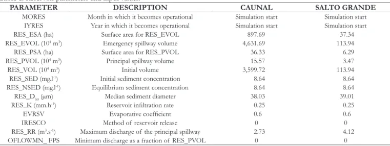
Table 1 shows the parameters required by the water release method adopted, and also the respective values used.
The data of RES_VOL, RES_PVOL, RES_EVOL, RES_PSA
and RES_ESA were obtained using the method of Triangulation with Linear Interpolation, employing bathymetric data surveyed by Lino et al. (2009), and altimetric data on a 1:10,000 scale of the Department of Sustainable Development of the state of Santa Catarina-BR.
For IRESCO the method of Average Annual Release Rate for Uncontrolled Reservoir was chosen, because it was the most appropriate to represent the type of anthropic operation performed in these dams. This method requires the value of RES_RR, referring to the maximum discharge for when the volume
is situated among the values defined for the main spillway and
the emergency spillway. The amount of water that exceeds the volume of the emergency spillway is released downstream. For the Caunal Dam, the mean of the estimated values of liquid discharge during the period from 2010 to 2014 (ZANIN; BONUMA; FRANCO, 2017), which is close to the 3rd quartile of the flow
data, was used. For Salto Grande Dam the Area Weighting method (STEDINGER; VOGEL; FOUFULA-GEORGIOU, 1992) was
used, based on the mean of the Caunal Dam flows, due to the
For RES_SED and RES_NSED of the reservoirs of both dams, the mean of 20 SSC samplings performed by Zanin, Bonuma and Franco (2017) in the Caunal Dam was used. The value of RES_D50 in the Caunal and Salto Grande reservoirs was obtained in the same way as the D50 of the channel banks, considering the
area of contribution of each reservoir. For EVRSV the default
value (0.6) was used, while for RES_K, which had an amplitude in the model from 0 to 1 mm.d-1, the value of 0.25 mm.d-1 was
arbitrarily inferred. The zero value was used as OFLOWMN_FPS considering the anthropic regulation of this dam, with an absence of discharge on some days.
Meteorological data
The daily rainfall data were obtained from 3 rain gauging stations located within the RPW (Figure 1). They are: (a) automatic
station CVG, which is under the responsibility of the Companhia Volta Grande de Papel (CVG) and; (b) conventional stations
Corredeira (Cod. 2649055) and Moema (Cod. 2649054) under the responsibility of ANA. Although 3 point sources of rainfall data are not highly representative of total rainfall resulting in a 965.8 km2 basin, each of these stations is located in one of the three
main sub-basins of the RPW, at altitudes of 845m (Corredeira),
880m (CVG) and 950m (Moema).
For the climate generator of SWAT, meteorological data representative of the region were inserted. These data were obtained from the Rio Negrinho meteorological station (Cod. A862 and former code 84), under the responsibility of the Instituto Nacional de Meteorologia (INMET, and formerly the responsibility of EPAGRI/INMET). This station is located close to the basin mouth, as shown in Figure 1, and includes a
22-year time series. Besides filling out the gaps in the rainfall
records of the conventional stations, the climate generator was used to simulate the meteorological data necessary to calculate evapotranspiration, because the meteorological station is outside the limits of the RPW.
It should be emphasized that in the case of the gap in the record of the extreme event that occurred in June 2014, it was not
completed by the model. In that case, the rainfall that occurred during the event, accumulated and recorded by the conventional stations on the last day of the phenomenon, was redistributed among the days in which the rainfall occurred, proportionally to
the records of the CVG automatic station.
Subdivisions of the RPW and main parameterizations
The criteria of Table 2 were adopted to define micro-basins and HRUs. For the micro-basins, since the level of sub-division affected the simulation of sediment yield (XAVIER et al., 2007),
the mean value identified by Fan et al. (2013) as a minimum contribution area for the generation of the hydrography for regions with porous hydrogeology and mean slope greater than 2.5% was used. After the drainage network was designed by the model, it was visually validated with the hydrography mapped on a scale of 1:50,000 (EPAGRI/IBGE, 2004).
The CN-SCS method (USDA, 1972) was used to calculate the generation of surface runoff, with a value adjusted for slopes greater than 5% (WILLIAMS, 1995). The Penman-Monteith method (MONTEITH, 1965; ALLEN, 1986; ALLEN et al., 1989) was used to calculate the evapotranspiration. The Muskingum method (BRAKENSIEK, 1967; OVERTON, 1966) was used for water routing in the river channel, considering its degradation, and the Yang Sand and Gravel method (YANG, 1996) for routing
sediments in a fluvial environment.
Warm-up, calibration and validation
For the appropriate warm-up of the model, it is recommended to utilize 2 to 3 years, with calibration and validation being performed in two different sections of the period of data observed, both of them bearing characteristics of wet and dry years. (ARNOLD et al., 2012a). In this way, the model was warmed up during the years of 2009 and 2010, and calibrated for the years of 2011 and 2012, with validation in 2013 and 2014.
Table 1. Reservoir parameters and input values.
PARAMETER DESCRIPTION CAUNAL SALTO GRANDE
MORES Month in which it becomes operational Simulation start Simulation start IYRES Year in which it becomes operational Simulation start Simulation start
RES_ESA (ha) Surface area for RES_EVOL 897.69 37.34
RES_EVOL (104 m3) Emergency spillway volume 4,631.69 113.94
RES_PSA (ha) Surface area for RES_PVOL 36.33 6.29
RES_PVOL (104 m3) Principal spillway volume 15.57 3.47
RES_VOL (104 m3) Initial volume 3,599.72 113.94
RES_SED (mg.l-1) Initial sediment concentration 8.64 8.64
RES_NSED (mg.l-1) Equilibrium sediment concentration 8.64 8.64
RES_D50 (µm) Median sediment diameter 38.03 39.01
RES_K (mm.h-1) Reservoir infiltration rate 0.25 0.25
EVRSV Evaporative coefficient 0.6 0.6
IRESCO Method of reservoir release 0 0
RES_RR (m3.s-1) Maximum discharge of the principal spillway 2.73 4.12
Defining a threshold for wet and dry years based on the
means of the annual totals of 10 years of liquid discharge and rainfall (Figure 3), it is found that model warm up was performed for a dry year (2009) and a normal to wet year (2010). On the other hand the calibration and validation periods comprise a dry year and a wet year each. Another form of calibration/validation recommended by Arnold et al. (2012a), is to adjust the parameters in a basin and validate them for the same period in another similar basin called Proxy Catchment Test by Klemes (1986).
In order to evaluate the simple and multi-site calibrations, the 3 procedures proposed by Moussa, Chahinian and Bocquillon (2007) were used. The first procedure is the evaluation of the uncalibrated model. In the second the model is calibrated only at the basin river mouth (Avencal station) for a data period (2011-2012), and validated with another data period at the same basin river mouth (2013-2014) and in the sub-basins (Caunal Dam). In the third procedure, multi-site calibration is performed (Avencal
station and the dams of Caunal and Salto Grande) for a data period (2011-2012), and validated in another period (2013-2014).
In the second procedure only the parameters referring to the water and sediment processes intrinsic to the watershed, and to the anthropic activities for the management of rural areas were calibrated. To perform the calibration, the base used was (a) the analysis of the water balance obtained in procedure 1, (b) the results of the study by Arnold et al. (2012a), and (c) the calibration values of Lino et al. (2009) (Table 3). The base used to calibrate sediment yield was (a) the analysis of the sediment balance with water balance calibrated in this procedure, and (b) the study by Arnold et al. (2012a) (Table 4). As a complement, other hydrological/sedimentologic studies with SWAT were also used (Table 5).
In the third procedure, the calibration performed previously was maintained, and only the hydrological and sedimentological
parameters of the artificial processes occurring in the watershed
Table 2. Criteria and results for micro-basin and HRUs generation.
PARAMETER VALUE
Cumulative Area for Hydrography (ha) 33
Slope Class 5
Slope Class Ranges (%)
0 a 5 5 a 10 10 a 20 20 a 30 >30
Threshold for HRUs*
Land Use (%) 10
Soil Type (%) 10
Slope (%) 10
Number of Microbasins 1,388
Number of HRUs 32,084
*When using multiple HRUs in the sub-basins it is possible to define the degree of spatial discretization of the HRUs. This depends on the relative or absolute area
of land use/cover in relation to the sub-basin area, the soil type over the land use/cover area, and slope over the soil type area.
were adjusted. These refer to the reservoirs of the Caunal and Salto Grande dams. Since Caunal Dam was the only one with observed hydrosedimentological data, it was used for evaluation. For the Salto Grande Dam the calibrations performed in the dam evaluated were repeated, because the initial values of the more uncertain parameters had been copied or extrapolated from the Caunal Dam. The base used to perform the calibration was (a) analysis of the water and sediment balance of the Caunal Dam obtained in procedure 2, and (b) other modeling studies with SWAT (Table 6).
Green and Van Griensven (2008) recommend the combination of the manual calibration with automatic calibration in the SWAT model. However, it was decided to use only manual calibration in
this study. This choice was due to the physical peculiarities of the
watershed, which can only be identified by the hydrologist (GREEN;
VAN GRIENSVEN, 2008; LUBITZ; PINHEIRO; KAUFMANN, 2013; MELO NETO et al., 2014; BROUZIYNE et al., 2017). According to Tucci and Collischonn (2003), for a user experienced in hydrological modeling, manual calibration is a relatively simple stage that implicitly takes multiple objectives into account. These authors also found that the results obtained with automatic multi-objective calibration are equivalent to those obtained with a good, detailed manual calibration. In agreement with these authors, it was found that in the results of Sloboda and Swayne (2013) the hydrological simulations with SWAT utilizing manual
calibration have the same level of efficiency as the simulations
Table 3. Most sensitive SWAT parameters for water balance in 64 modeling studies ascertained by Arnold et al. (2012a), and calibration values of Lino et al. (2009) for the RPW.
SURFACE RUNOFF Lino et al. (2009) BASE FLOW Lino et al. (2009)
CN2 -13% to -20%; +2% ALPHA_BF 1
SOL_AWC * GW_REVAP *
ESCO 0 GW_DELAY 10
EPCO * GW_QMN *
SURLAG 0 REVAPMN *
OV_N * RCHRD_DP *
*Not calibrated by Lino et al. (2009).
Table 4. Most sensitive SWAT parameters for sediment balance in 64 modeling studies ascertained by Arnold et al. (2012a).
LANDSCAPE CHANNEL
USLE_P PRF
USLE_C APM
USLE_K SPEXP
LAT_SED SPCON
SLSOIL CH_EROD
SLOPE CH_COV
Table 5. Other parameters with sensitivity and/or calibrated in SWAT modeling studies.
PAR. H. CAL. L.B. REFERENCE
CANMX 42 NB Malutta (2012); Souza and Santos (2013); Brighenti, Bonuma and Chaffe (2016)
BLAI 43% Vietnam Emam et al. (2016)
SOL_K 900% NB; SC Malutta (2012); Lubitz, Pinheiro and Kaufmann (2013)
CH_N 141% USA; BV Tuppad et al. (2010); Brighenti, Bonuma and Chaffe (2016)
MSK_CO1 1,100% Africa Schuol and Abbaspour (2006)
MSK_CO2 2,300%
CH_COV1 0.6* USA; SF Tuppad et al. (2010); Creech et al. (2015)
SOL_BD ** Lenhart et al. (2002)
CHBNK_D50 500 USA; SF Jeong et al. (2011); Creech et al. (2015)
CHBED_D50 500
CHBNK_KD 0.1 SF; Iran Creech et al. (2015); Garizi and Talebi (2016)
CHBED_KD 1.0
CHBNK_TC 200.6 SF; Iran Creech et al. (2015); Garizi and Talebi (2016)
CHBED_TC 257.4
The percentages refer to the difference between the initial value and the calibrated value in relation to the initial value. The absolute values refer to the value added when the initial value is zero. PAR. = Parameter; H. CAL. = Higher Calibration among the referenced studies; L.B. = Location of the Basin; NB: Neighboring Basin
calibrated with the main algorithms of SWAT-CUP. The only
significant difference found by these authors was the time of
execution. On the other hand, Melo Neto et al. (2014) identified
manual calibration as more efficient than automatic calibration.
These authors found a cascade effect of incoherent values in the automatic calibration process, where one parameter compensates for the other, generating simulations with values close to the real ones, but without representing the dominant physical processes in the basin. It should be underscored that some SWAT users have been choosing only manual calibration in recent years, obtaining satisfactory simulations (LUBITZ; PINHEIRO; KAUFMANN, 2013; BROUZIYNE et al., 2017). In this way it was found that the great advantage of automatic calibration is that it saves time, while manual calibration is essential to ensure the appropriate representation of the physical processes in the watershed. The use of automatic calibration, restricted to a small amplitude around the manually calibrated values, would probably result in a slight gain in the statistical indices. However, since the objective of this study is to evaluate the simple and multi-site calibrations in
the watershed, manual calibration was sufficient to compare the
different procedures that are being analyzed.
In the manual calibration process, the different parameters were adjusted individually and cumulatively, and the changes in the values were done similarly with the analysis of manual sensitivity by Lubitz, Pinheiro and Kaufmann (2013). In other words,
each of the parameters identified in the literature was altered at
constant intervals (generally 5%) on their initial values, until the best calibration was obtained. The range of the adjustments was limited arbitrarily, according to the uncertainties contained in the initial value of each parameter.
Different evaluation metrics were used to assess the efficiency
of the simulations, aiming to verify the performance of the model in different parts of the hydrograph. For peak events, the index of Nash and Sutcliffe (NSE) (NASH; SUTCLIFFE, 1970) and the
coefficient of determination (R2) (MONTGOMERY; RUNGER,
2003) were used, since they are more influenced by the maximum values (MORIASI et al., 2007). The Mean Absolute Error (MAE) was used for mean values, showing the central tendency value of the error in simulation in the same units as the data observed, and the Percentage Bias (PBIAS), which enables evaluating the mean tendency of the simulated volumes (MORIASI et al., 2007). For the minimum events, the LogNSE index was used, which is applied in hydrology studies for this purpose (SOUZA; SANTOS, 2013).
Although the developers of the SWAT model (ARNOLD et al., 2012a) consider daily simulations of streamflow and sediments
with values ≥ 0.5 and 0.6 for NSE and R2, respectively, acceptable,
this study adopted other individual criteria for each basin.
In the 6th order river basin, the criterion of Green et al. (2006)
was adopted. They considered satisfactory daily simulations in
SWAT with values ≥ 0.4 and 0.5 for NSE and R2, respectively, in
a predominantly rural basin on a mesoscale (580.5 km2). On the
other hand, for the reservoir that is the mouth of the 5th order
river basin, the criterion of Kim and Parajuli (2014) was adopted. When they evaluate the module of SWAT reservoirs in the daily time step, they consider values of NSE and R2 ≥ 0.3 acceptable. The choice of these values is justified for the indices mentioned
for the following reasons: a) there are two representative reservoirs
in the main river of the RPW, and this limits the efficiency of the
hydrological simulations of the SWAT model (ZHANG et al., 2013), reducing the inter-annual sedimentological variability in dammed rivers (VIGIAK et al., 2017); b) Wu and Chen (2012) calibrating the daily liquid discharge in 3 methods of release from reservoirs in the SWAT model, obtained an NSE of 0.13 to 0.36 and
correlation coefficient (r) of 0.36 to 0.60 during the calibration
period, with smaller values during the validation period; and c) the aforementioned criteria meet the objective of evaluating different modeling procedures in nested basins.
For PBIAS, Moriasi et al. (2007) recommend values
of < ± 25% and < ± 55% for streamflow and sediments,
respectively, in monthly simulations on watersheds. Thus, for the daily time step, and considering also the analysis of reservoirs,
in this study values of < ± 30% for streamflow and < ± 60%
for sediments will be considered valid. For MAE, Moriasi et al. (2007 and references therein) consider values less than 50% of the standard deviation of the data observed.
According to a recommendation by Zeiger and Hubbart (2016), first the liquid discharge was calibrated and then the solid discharge, because the hydrological processes were dominant in sediment yield (VAN GRIENSVEN et al., 2006). Aiming to perform a more realistic calibration of the water balance, as per the recommendation by Yu and Schwartz (1999), together with the
total runoff, the surface runoff and base flow were also evaluated.
These were obtained by separating the runoff with the Base Flow Filter algorithm (ARNOLD et al., 1995a).
As to the sedimentological calibration, the channel parameters present the greatest uncertainties (ARNOLD et al., 2012a). Moreover, if the Yang Sand and Gravel method is used, the parameterizations
of the channels are even more influential in the production
of sediments than those of landscape (JEONG et al., 2011). Nevertheless, the input of sediments to the channels affects the
fluvial sedimentological processes, since it directly influences
the SSC (HUDSON-EDWARDS, 2007 and references therein).
Thus, first the parameters referring to landscape processes were
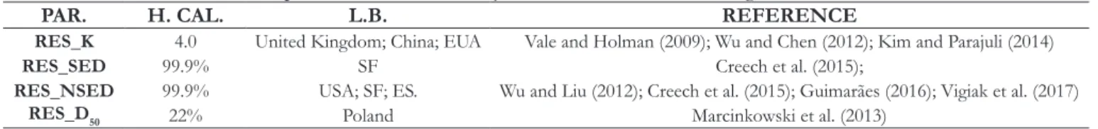
calibrated and then those of the channels. Table 6. SWAT reservoir module parameters with sensitivity and/or calibrated in modeling studies.
PAR. H. CAL. L.B. REFERENCE
RES_K 4.0 United Kingdom; China; EUA Vale and Holman (2009); Wu and Chen (2012); Kim and Parajuli (2014)
RES_SED 99.9% SF Creech et al. (2015);
RES_NSED 99.9% USA; SF; ES. Wu and Liu (2012); Creech et al. (2015); Guimarães (2016); Vigiak et al. (2017)
RES_D50 22% Poland Marcinkowski et al. (2013)
Only the hydrological parameters used in the IRESCO=O. With the exception of Vigiak et al. (2017), the sedimentological studies carried out the evaluation in
RESULTS AND DISCUSSION
Fluviometric data
When filling out the gaps in the water level records of
Avencal station, the regression model used based on the data from Rio Preto do Sul station obtained an R2 of 0.53. The periods in which gaps were filled out with this regression model were only
used in Figures 3 and 4. On the other hand, the regression model
based on data from the Rio da Várzea dos Lima station obtained
an R2 of 0.73 and overestimates on average 29% of the data
observed. Only this model was used to complete the gaps in the evaluation period of this modeling, more precisely, the days of the
peaks of the extreme event in June/2014. The level-streamflow rating curves of the RPW, defined for the levels below and above
194 cm, have an R2 of 0.80 and 0.88, respectively. The rating
curve of total solid discharge from this basin, on the other hand, obtained an R2 of 0.90.
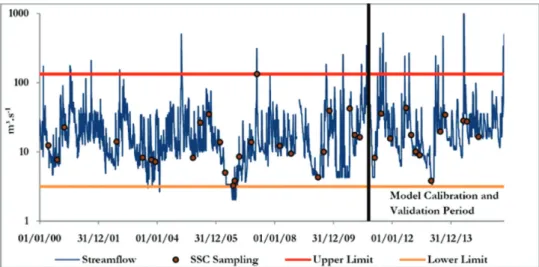
Figure 4 shows the SSC sampling campaigns on the hydrograph of Avencal station, and the limit of extrapolation
of the streamflow rating curve. It is observed that during the period from 2000 to 2014, the streamflow rating curve was only
extrapolated in a few minimum extreme events, and in most of the maximum extreme events. However, the SSC sampling campaigns
were performed predominantly during flows with intermediate
magnitudes, with few samplings during extreme events. Based on the hydrograph events, it was found that the 38 SSC sampling campaigns covered all its moments, and most of the samples are located in the recession (17 records) and rise (9 records) of the hydrograph, and there are also 7 samplings over the valley and
5 samplings over streamflow peaks. For the Caunal Dam, the
liquid discharge-suspended solid discharge rating curve has an R2 of 0.95. The SSC samplings on the hydrograph of this dam, and also their classification by event, may be verified in Zanin, Bonuma and Franco (2017).
1° Modeling procedure: initial simulation
According to Table 7, the initial simulation was not satisfactory for the RPW and the Caunal Dam. This is due to
the poor performance of the base flow, resulting in a streamflow
equal to 0 m3.s-1 on some days of the simulated hydrograph
(not shown). In the PBIAS values except for the surface runoff during the calibration period, all runoffs were underestimated in both periods in the RPW. In the Caunal Dam, the simulations overestimate the data observed.
Although the hydrological simulation was not satisfactory, the sediment yield simulation was examined (Table 8). As expected, the simulations were not satisfactory in both basins. For the RPW,
while the sediment yield is overestimated in the first period of
evaluation, it is underestimated in the second period. But in Caunal Dam it is underestimated in both periods.
2° Modeling procedure: simple calibration
The calibration of the RPW water balance aimed to
reduce the water losses, increasing base flow. Table 3 shows
that the parameters identified by Lino et al. (2009) as the most
influential in the RPW water balance corroborate the study by
Arnold et al. (2012a). Nevertheless, observing the values used in the calibration by Lino et al. (2009), it was found that the base
flow recession constant (ALPHA_BF) and the surface runoff lag coefficient (SURLAG) do not represent the physical characteristics
of the RPW, since the value of ALPHA_BF equal to 1 (1 day) is much lower than the value of 0.0313 (approx. 40 days) calculated
based on observed RPW streamflow data. Likewise, a SURLAG
value equal to zero indicates that no fraction of the surface runoff reaches the main channel on the day when it is generated, which is not compatible with the concentration time of 18.98h of the RPW.
The need for excessive adjustment of the SWAT parameters, to render the simulated data compatible with the observed data, forcing the simulation of the physical processes in the model,
was already found by Lubitz, Pinheiro and Kaufmann (2013) and Melo Neto et al. (2014). Therefore, the calibration by Lino et al. (2009) was considered only for the identification of the more sensitive parameters.
Since the simulation of surface runoff, except for R2,
was satisfactory for the other indices for the 1st procedure
(Table 7), it was not necessary to perform a calibration using the
coefficient of generation of surface runoff for the condition of
mean moisture of the soil (CN2). Besides, since the shape of the simulated hydrograph is in accordance with the shape of the observed hydrograph (Not shown), it was not necessary to adjust
the Manning value for overland flow (OV_N) and the SURLAG.
The parameter ALPHA_BF was also not adjusted, since its initial value was extracted from the observed hydrograph.
Aiming to reduce water losses to the atmosphere, the compensation factor of evaporation from the soil (ESCO) was increased to the maximum, since in this way only the surface layer of the soil meets the evaporative demand of the low troposphere. The compensation factor of water uptake from soil by the plants (EPCO) was not sensitive to calibration, which is due mainly to
the fact that the root zone is comprised of the entire soil profile.
The reduction of EPCO, associated with the reduction of the root zone or with the increased soil depth, did not improve the simulation in any way. The water content available to plants (SOL_AWC) was reduced by 50%, diminishing plant transpiration. Besides these parameters, the value of maximum canopy storage of plants (CANMX) and the maximum leaf area index (BLAI) were reduced by 25% and 50%, respectively.
Table 7. Statistical indices of the three hydrological modeling procedures.
P FLOW AVENCAL CAUNAL
NSE R2 PBIAS MAE LogNSE NSE R2 PBIAS MAE LogNSE
1° PROCEDURE (INITIAL SIMULATION)
C BF. -0.01 0.38 62.78 15.05 -7.47 - - - -
-SR. 0.59 0.17 -0.59 9.26 0.47 - - - -
-TF. 0.54 0.41 42.31 18.62 -2.35 0.19 0.26 -59.69 3.10 -0.06
V BF. 0.00 0.28 79.91 19.28 -15.85 - - - -
-SR. 0.46 0.06 47.50 13.86 0.49 - - - -
-TF. 0.38 0.26 67.14 29.21 -6.44 0.91 0.02 -65.85 1.81 -0.29 2° PROCEDURE (SIMPLE CALIBRATION)
C BF. 0.62 0.78 31.12 8.25 0.10 - - - -
-SR. 0.57 0.30 0.86 8.99 0.58 - - - -
-TF. 0.62 0.75 21.34 13.63 0.57 0.02 0.32 -96.77 4.06 -0.29
V BF. 0.24 0.50 57.25 14.33 -0.95 - - - -
-SR. 0.50 0.13 41.27 13.29 0.55 - - - -
-TF. 0.46 0.53 50.95 24.32 0.19 0.67 0.00 -124.94 2.76 -0.46 3° PROCEDURE (MULTI-SITE CALIBRATION)
C BF. 0.57 0.76 35.85 9.03 -0.08 - - - -
-SR. 0.57 0.29 5.38 8.80 0.57 - - - -
-TF. 0.61 0.74 26.00 13.93 0.50 0.30 0.30 -43.12 2.77 0.02
V BF. 0.21 0.46 60.85 14.98 -2.55 - - - -
-SR. 0.47 0.14 45.60 13.35 0.55 - - - -
-TF. 0.43 0.45 54.84 24.97 -0.53 0.86 0.04 -41.62 1.41 -0.09 Values within the adopted criteria are highlighted. C = Calibration (2011-2012); V = Validation (2013-2014); BF. = Base Flow; SF. = Surface Runoff; TF. = Total Flow (Streamflow); P=Period.
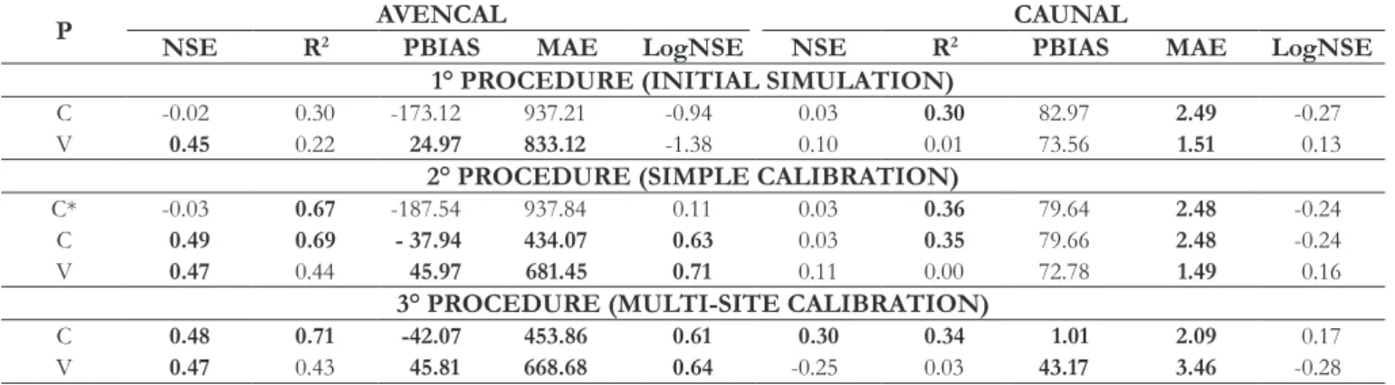
Table 8. Statistical indices of the three sedimentological modeling procedures.
P AVENCAL CAUNAL
NSE R2 PBIAS MAE LogNSE NSE R2 PBIAS MAE LogNSE
1° PROCEDURE (INITIAL SIMULATION)
C -0.02 0.30 -173.12 937.21 -0.94 0.03 0.30 82.97 2.49 -0.27
V 0.45 0.22 24.97 833.12 -1.38 0.10 0.01 73.56 1.51 0.13
2° PROCEDURE (SIMPLE CALIBRATION)
C* -0.03 0.67 -187.54 937.84 0.11 0.03 0.36 79.64 2.48 -0.24
C 0.49 0.69 - 37.94 434.07 0.63 0.03 0.35 79.66 2.48 -0.24
V 0.47 0.44 45.97 681.45 0.71 0.11 0.00 72.78 1.49 0.16
3° PROCEDURE (MULTI-SITE CALIBRATION)
C 0.48 0.71 -42.07 453.86 0.61 0.30 0.34 1.01 2.09 0.17
V 0.47 0.43 45.81 668.68 0.64 -0.25 0.03 43.17 3.46 -0.28
To increase the base flow, the delay time of groundwater flow (GW_DELAY) was reduced to half of the value calibrated
by Lino et al. (2009), associated with the 75% reduction of the water threshold in the shallow aquifer for the occurrence of
base flow (GW_QMN). The water fraction that percolates from
the shallow aquifer to the deep aquifer (RCHRG_DP), was also reduced. Due to the porous hydrogeology of the RPW (CPRM, 2007), it was considered arbitrarily that the minimum acceptable value was 2%.
The capillary rise coefficient of water in soil (GW_REVAP),
and the water threshold in the shallow aquifer for the water rise
to occur (REVAPMN), were not sensitive to calibration. To make it easier to infiltrate into the soil and increase the groundwater flow, the saturated hydraulic conductivity of soils (SOL_K) was
increased by 25%.
In order to correct the absence of streamflow on some days, the Manning coefficient (CH_N) was reduced by 40%, increasing the flow rate. Since CH_N is based on the channel cover, it was
considered necessary to also reduce the cover factor of the banks
(CH_COV1) and bed (CH_COV2), since these parameters affect the degradation of the channel and consequently river flow.
The calibration coefficients of the normal (MSK_CO1) and minimum (MSK_CO2) flow storage time constant of the
Muskingum method, were raised to 2 and 10, respectively. In this way the storage time of the constant value along the different channel segments increased. Table 9 presented a summary of the water balance calibration performed in this procedure.
The simulation of total flow was satisfactory with the
aforementioned calibration, according to Table 7. This is due
mainly to the significant improvement of the base flow that,
although not yet satisfactory, achieved better values in all metrics, with three acceptable indices. The surface runoff was maintained with acceptable values in four indices, improving the values of
three of the five metrics.
In the validation period, the simulation of total flow was not satisfactory, despite the significant improvement in relation to the initial simulation. The streamflow simulated in this period
obtained three acceptable indices, and was not accepted because
of strong underestimation, due to the poor representation of the
minimum flows, according to the values of PBIAS and LogNSE. Once the total flow has been calibrated, Table 8 shows that the simulation of sediment yield is unsatisfactory in the RPW. Since the value of PBIAS is strongly overestimated the sedimentological calibration aimed at reducing the estimate of erosive processes in the RPW. The factor of conservationist practices of MUSLE (USLE_P) in areas with agriculture and
exposed soil, was reduced by 50%, confirming the minimum values
tabulated by Wischmeier and Smith (1978). The minimum value of the water erosion factor based on soil cover (USLE_C) was reduced by 50% for agriculture and exposed soil, due to lack of knowledge regarding the types and amounts of crops cultivated in the RPW. It was also necessary to reduce the soil erodibility factor of the MUSLE (USLE_K) by 25%.
As to the sediment concentration in lateral and groundwater
flow (LAT_SED), its default value is already the minimum (value 0). However the length of the lateral ramp for the sub-surface flow
(SLSOIL), as well as the mean slope (SLOPE), were extracted directly from HCDEM by SWAT model, and therefore they were not adjusted. The bulk density of the soils (SOL_BD) was reduced by 25%.
The adjustment factor of sediment transport with the
peak flow in the main channel (PRF) did not present sensitivity in
calibration. The default value of the same factor for tributary channels (APM or ADJ_PKR) was reduced by 50%. This calibration is due
to the absence of linearity between SSC and streamflow in the data
from Avencal station. The linear (SPCON) and exponential (SPCON)
coefficients of Bagnold’s sediment transport were not altered since
this method was not utilized in this modeling. The monthly erodibility parameter of the channel (CH_EROD) did not present sensitivity, as occurred with Lubitz, Pinheiro and Kaufmann (2013). As to the
parameter of banks and bed cover (CH_COV), this has already
been adjusted in the calibration of liquid discharge.
The D50 of the banks (CH_BNK_D50) and bed (CH_BED_D50) was increased by 25%. On the other hand, the bulk density of the banks (CH_BNK_BD) and bed (CH_BED_BD) was reduced by 25%. The critical shear stress values of the banks (CH_BNK_TC)
Table 9. Manual calibration of the RPW water balance.
PARAMETER INITIAL VALUE OPERATION OPERATION VALUE FINAL VALUE
ESCO 0.95 Replacement 1 1
SOL_AWC Several Multiplication 0.50 Several
CANMX 3.40 FRST
2.71 PINE
Multiplication 0.75 2.55
2.0325
BLAI Several Multiplication 0.50 Several
GW_DELAY 31 Replacement 5 5
GW_QMN 1,000 Multiplication 0.25 250
RCHRD_DP 0.05 Multiplication 0.20 0.01
SOL_K Several Multiplication 1.25 Several
CH_N(1,2) 0.05 Multiplication 0.60 0.03
CH_COV(1) 5.40 Multiplication 0.60 3.24
CH_COV(2) 1.97 Multiplication 0.60 1.182
MSK_CO1 0.75 Replacement 2 2
and bed (CH_BED_TC) were increased 4 times. Therefore, the erodibility according to the jet test of the banks (CH_BNK_KD) and bed (CH_BNK_KD), which was estimated based on the critical shear stress, was calculated again based on the calibrated values. These calibrations whose initial value was greatly altered
are justified because the initial values are estimated from the bank
and bed cover. Table 10 presents a summary of the calibration of sediment yield.
As a result of the calibrations, the sedimentological simulation of the RPW was satisfactory during the calibration period (Table 8). This simulation was not validated only because of the value of R2, which despite being close to the criterion adopted was not
satisfactory. It should be pointed out that while the calibration period overestimates the data observed, the validation period underestimates them. When the sediment balance was calibrated, especially the parameter SOL_BD, variations occurred that were smaller than or equal to a unit in the hydrological calibration evaluation indices, and the metrics of acceptable values were maintained in criterion adopted.
Analyzing the simulations of this procedure in the nested basin (Tables 7 and 8), it is found that neither simulation was satisfactory. Except for R2 in the calibration period, the hydrological
adjustments in the watershed made the values of the other metrics worse in both evaluation periods. On the other hand, the sedimentological calibration of the RPW slightly improved the values of most metrics of the Caunal Dam. For this reason it was not possible to perform the hydrosedimentological validation by Proxy Catchment Test in the RPW.
3° Modeling procedure: multi-site calibration
The liquid discharge of the Caunal Dam did not show good results in the previous procedures, and the data observed were greatly overestimated (Table 7). Thus, the calibration of the water balance aimed at increasing the water losses in the reservoirs.
The initial value of RES_K was inferred arbitrarily, and was very imprecise. Another parameter full of uncertainties is
EVRSV, in which the default value of the model was used. It was
thus necessary to increase the value of RES_K by 4.4 times its
initial value, associated with the maximum value of EVRSV, to
obtain an acceptable water balance.
Another parameter with many uncertainties is RES_VOL.
Figure 3 shows that the year the simulation began (2009) was a dry year and the year that the records of Caunal Dam began (2010) was
a wet year. The accumulated rainfall (Station CVG) in the previous
month (12/2008) when the simulation began was 90.4 mm, and
the streamflow on the day the simulation began (01/01/2009) at
the mouth of the RPW was 8.57 m3.s-1. Meanwhile, the value used for RES_VOL (referring to 01/01/2009) in the Caunal Dam was
the volume of day 01/01/2010, in which the accumulated rainfall
of the previous month (12/2009) was 158 mm, with a streamflow
of 23.47 m3.s-1 at the mouth of the RPW on the aforementioned day. Thus, in order to render compatible the value of RES_VOL
obtained in the wet year (2010) with a more representative value of the dry year (2009), the value of this parameter was reduced by 50%. Another parameter that had to be adjusted was RES_RR,
and its reduction by 15% was justified because the initial value
was based on the mean of the daily sample of the liquid discharge from a dam between 2010 and 2014.
As to the Salto Grande Dam, while the Caunal Dam reservoir is located predominantly on Medium Texture Haplic Cambisol (average SOL_K of 66.415 mm.h-1), the Salto Grande reservoir is located predominantly on Clayey/Very Clayey texture Haplic
Nitosol (average SOL_K of 23.395 mm.h -1). For this reason, it was assumed that the losses by infiltration in this reservoir are
smaller than those from the reservoir of the Caunal Dam, and the initial value was rounded off to 0.3 mm.h-1. As to the parameter EVRSV, due to the closeness of the 2 reservoirs, the atmospheric
conditions are practically the same, thus the maximum value of this parameter was also adopted. Since the volume of the Salto Grande Dam is always kept at the maximum level, without any discharge from the emergency spillway, due to the fact that its
inflow is regulated by the anthropic operation of the Caunal
Dam (dam operator, personal communication in 2014), the initial volume of the Salto Grande Dam was not altered. On the other hand, the value of RES_RR, which was obtained by weighting areas based on the value of this parameter for the Caunal Dam, was also reduced by 15%.
With this calibration all metrics had better values (Table 7).
However, only the simulations of maximum flows were acceptable
based on the values of NSE and R2, and also the mean volume
discharged by the dam due to the value of MAE. Although the Table 10. Manual Calibration of the RPW Sediment Yield.
PARAMETER INITIAL VALUE OPERATION OPERATION VALUE FINAL VALUE
USLE_P Several* Multiplication 0.50 Several*
USLE_C 0.20* Multiplication 0.50 0.10*
USLE_K Several Multiplication 0.75 Several
SOL_BD Several Multiplication 0.75 Several
ADJ_PKR 1 Multiplication 0.50 0.50
CH_BNK_D50 61.04 Multiplication 1.25 76.30
CH_BED_D50 95.37 Multiplication 1.25 119.2125
CH_BNK_BD 1.19 Multiplication 0.75 0.8925
CH_BED_BD 1.49 Multiplication 0.75 1.1175
CH_BNK_TC 73.23 Multiplication 4 292.92
CH_BED_TC 19.44 Multiplication 4 77.76
CH_BNK_KD 0.0234 Re-estimated 0.0117 0.0117
CH_BED_KD 0.0454 Re-estimated 0.0227 0.0227
overestimate presented in the PBIAS value was reduced by more than half in relation to the previous procedure, and the value of LogNSE became greater than zero, these two indices remained unsatisfactory. During the validation period, the values of the metrics improved in relation to the previous procedure, but only two were acceptable.
Due to the hydrological calibration, the underestimate of the sedimentological simulation of the reservoir increased, worsening its evaluation indices. Thus, the sediment balance calibration aimed at increasing the estimate of the solid discharges, diminishing the estimate of sediment deposition.
Since parameter RES_D50 presented low sensitivity to calibration, its initial value was not altered. Only parameters RES_NSED and RES_SED were adjusted together, since the
individual adjustments proved inefficient. In order to improve the
value of the evaluation metrics, it was necessary to increase the initial value of these parameters by 32 times, considering that the smaller adjustments presented little sensitivity. This excessive increase is
justified in the case of RES_NSED, by the great uncertainty in its
initial value, in which the mean value of SSC was used, obtained by point samplings performed by Zanin, Bonuma and Franco (2017). Now, for parameter RES_SED, in which the same initial
value of RES_NSED was used, this excessive increase is justified,
because of the reduction of the initial volume of the reservoir performed in the calibration of the water balance. Thus, there is less dilution of the sediment in aqueous medium, increasing the concentration. For the Salto Grande Dam the same values of the sedimentological parameters of the Caunal Dam were adopted. Table 11 shows the summary of the water and sediment balance calibrations of the two dams.
With these adjustments it was possible to improve the values of the metrics during the calibration period, and four acceptable indices were obtained. The sedimentological simulation was only not satisfactory due to the value of LogNSE, which despite being positive is not acceptable. On the other hand, in the validation period, while the values of R2 and PBIAS improved, in the other
metrics they became worse (Table 8).
The hydrological calibrations of the reservoirs impaired
the flow routing toward downstream, increasing the underestimate
in the RPW, and slightly impairing all indices. The metrics of satisfactory values in the previous procedure were maintained as such during the calibration period, while in the validation period
LogNSE and R2 were more affected, and the latter was no longer
satisfactory. As to the production of sediments by the RPW, the calibration of the reservoirs minimally affected the evaluation indices, increasing the overestimation during the calibration period and reducing the underestimation during the validation period (Tables 7 and 8).
Comparison of modeling procedures
In this topic, the 3 modeling procedures performed in this study are compared. Due to the better evaluation indices during the calibration period, the wet year of 2011 and the dry year of 2012 were analyzed. Figure 5 shows that the worst simulation of the water balance in both years for the RPW was that of the 1st procedure, as expected. This occurs both because of the
underestimate of the total volume and the proportion of base
and surface flows in the composition of the total flow, due to the
inversion of the pattern observed, with the surface runoff being
greater than the base flow. The 2nd and 3rd procedures, however,
provided a better representation of the data observed. They have
the same pattern of proportions of base and surface flows
observed, despite maintaining the underestimate which is slightly larger in the 3rd that in the 2nd procedure. As to these flows, it is important to observe that while the base flow is underestimated
in both years, the surface runoff is underestimated in the wet year and overestimated in the dry year. In general, it is found that the
simulations of total flow for the dry year were better than in the
wet year. On the other hand, the simulation of the wet year was better to represent the proportion of surface runoff and base
flow in the composition of the total flow.
The main deficiency of this modeling lies in the representation of base flow. Underestimates of hydrological simulations using
SWAT for dry years were also found by Brighenti, Bonuma and Chaffe (2016) and Lubitz, Pinheiro and Kaufmann (2013), but with overestimates for the wet years. On the other hand, Green
and Van Griensven (2008) found overestimates of dry periods and underestimates of wet periods. According to Kavetski, Kuczera and Franks (2006), it can be inferred that the underestimates may be due to the input and evaluation data of the model. In the modeling of the RPW, these limitations would be a) spatial limitation
of the rainfall data, or b) quality of the streamflow rating curve.
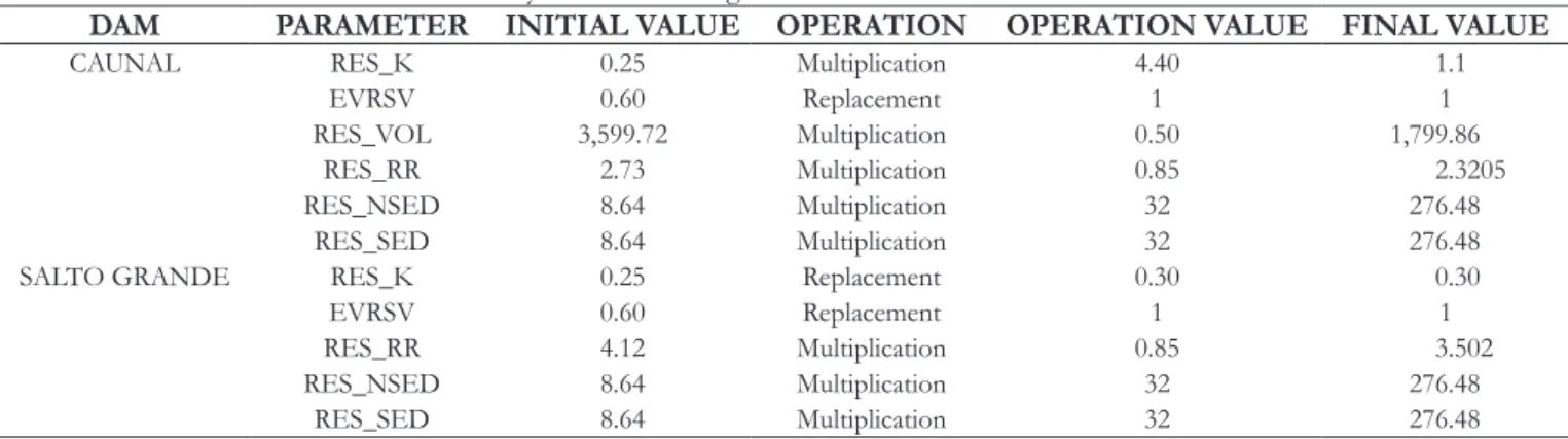
Table 11. Manual calibration of reservoirs hydrosedimentological balance.
DAM PARAMETER INITIAL VALUE OPERATION OPERATION VALUE FINAL VALUE
CAUNAL RES_K 0.25 Multiplication 4.40 1.1
EVRSV 0.60 Replacement 1 1
RES_VOL 3,599.72 Multiplication 0.50 1,799.86
RES_RR 2.73 Multiplication 0.85 2.3205
RES_NSED 8.64 Multiplication 32 276.48
RES_SED 8.64 Multiplication 32 276.48
SALTO GRANDE RES_K 0.25 Replacement 0.30 0.30
EVRSV 0.60 Replacement 1 1
RES_RR 4.12 Multiplication 0.85 3.502
RES_NSED 8.64 Multiplication 32 276.48