UNIVERSIDADE DO ALGARVE
FACULDADE DE CIÊNCIAS DO MAR E DO AMBIENTE
Migration and distribution of the veined squid Loligo forbesi in
Scottish (UK) waters
MAFALDA VIANA
Masters in Marine Biology (Fisheries and Aquaculture specialization)
UNIVERSIDADE DO ALGARVE
FACULDADE DE CIÊNCIAS DO MAR E DO AMBIENTE
Migration and distribution of the veined squid, Loligo forbesi, in
Scottish (UK) waters
MAFALDA VIANA
Masters in Marine Biology
(Fisheries and Aquaculture specialization)
Thesis developed in the University of Aberdeen:
Supervisor: Doctor Graham Pierce (SBS, University of Aberdeen)
Advisor: Doctor Manuel Afonso Dias (FCMA, Universidade do Algarve)
FARO (2007)
The author wishes to express her enormous gratitude to Dr. Graham Pierce for the opportunity and outstanding guidance and comments during this project and to University of Aberdeen that kindly had me. I also would like to thank Dr. Manuel Afonso Dias for placing me in the right direction before and during the thesis project, Dr. Janine Illian for the very helpful statistical advices, Dr. Colin MacLeod for the survey data supply and comments on the report and Dr. Jianjun Wang for the fishery and environmental data supply. Finally I wish to thank Marta Serpa Pimentel and Diogo Viana for sponsoring my studies and work.
Abstract
In order to protect and sustainably managefishery resources, it is essential to understand the temporal and spatial utilization of habitats of the target species. A Geographic Information System and length frequency analysis were used, in both fishery and survey data, to detect Loligo forbesi migration patterns from west to east coast of Scotland and inshore-offshore movements. Although the migration between west coast and North Sea is not evident, it is possible that veined squid performs an inshore movement in summer/autumn and offshore in winter/spring to complete their life cycle. Two distinct migratory behaviours between the two cohorts of Scottish veined squid is also a possibility, one cohort can be resident in inshore waters while the other migrates to offshore waters in winter and spring. The environmental reasons for such movements were examined using a generalized additive mixed model (GAMM) that suggested that distance to coast is the most important variable affecting size distribution in almost all seasons; however abundance distribution seems to be influenced with the same importance by sea surface temperature, depth and distance to coast. L. forbesi also revealed an optimal peak of abundance in waters at ~11oC, 200m depth and 25miles far from coast.
Key words: L. forbesi, temporal and spatial distribution, GAMM, environmental variables.
Resumo
De modo a proteger e gerir de forma sustentável os recursos pesqueiros é essencial compreender como as espécies alvo utilizam os seus habitats temporal e espacialmente. Na lula riscada (Loligo forbesi) da Escócia isto é bastante importante uma vez que não existe qualquer medida de gestão da sua pesca, além do tamanho mínimo da malha das redes de arrasto. L. forbesi, encontra-se principalmente em águas costeiras, e nas águas escocesas apresenta duas coortes com dois períodos de desova e duas épocas de recrutamento. Diferentes estudos demonstraram que várias espécies de lulas fazem migrações de curta escala, de perto para longe da costa, e de grande escala, Este-Oeste ou Norte-Sul, e.g. a L. forbesi de Inglaterra. Estas movimentações poderão ser causadas por condições ambientais, nomeadamente pela temperatura e pela profundidade, uma vez que a abundância de várias espécies de lulas é influenciada por estas mesmas condições ambientais. Deste modo, os objectivos da presente tese são (1) verificar se L. forbesi faz migrações da costa Oeste para a costa Este da Escócia, no Inverno, para desovar e da costa Este para a Oeste, na Primavera, tal como sugerido por estudos anteriores; (2) detectar as eventuais migrações da L. forbesi da Escócia para zonas afastadas da costa e caso estes movimentos existam, verificar qual a sua relação com o ciclo de vida da espécie e; (3) verificar quais as razões ambientais que levam as lulas a migrar, dando ênfase à sua relação com a temperatura superficial do mar (SST), profundidade e distância à costa.
Para testar as hipóteses, foram utilizados dados de cerca de 20 anos da espécie L. forbesi, fornecidos pelo Fisheries Research Services, provenientes de desembarques comerciais e de navios de investigação. Estes foram primeiro utilizados num Sistema de Informação Geográfica (SIG) e em análises de frequência de comprimentos para verificar a existência de uma migração entre a costa Este e Oeste da Escócia. Estas análises demonstraram que a migração entre a costa Oeste e Este não é evidente, mas comportamentos migratórios diferentes entre coortes podem ocorrer, uma vez que alguns dos mapas de SIG exibem dois picos distintos de abundância em certos anos e meses. Outra explicação pode ser que a
população de L. forbesi de Inglaterra, migre em certos anos mais para Norte que o habitual entrando no território escocês devido a condições ambientais mais favoráveis. Os mesmos dados foram utilizados para construir gráficos de abundância e frequência de comprimentos contra a distância à costa onde os arrastos foram feitos. Estes gráficos mostram que é possível que esta espécie migre para águas costeiras no Verão e Outono e para águas mais longínquas durante o Inverno e Primavera, com a finalidade de completar o seu ciclo de vida. A coorte que desova no Verão deverá fazê-lo em zonas costeiras assim como o seu recrutamento no Outono. Contudo, o local de desova da coorte de Inverno e as áreas de recrutamento na primavera não são claros. A hipótese de dois comportamentos migratórios distintos entre as duas coortes de L. forbesi da Escócia é também uma possibilidade: enquanto uma coorte é residente em águas costeiras a outra migra para longe da costa durante o Inverno e a Primavera, ou chega a estas águas longe da costa vindo de áreas ainda mais distantes como os Rockall Banks.
As razões ambientais para tais movimentos foram examinadas em R, com um modelo aditivo generalizado misto (GAMM), uma extensão do GAM, e com uma componente temporal (ano) como variável aleatória. Esta análise demonstrou que a distância à costa é a variável mais importante a afectar a distribuição por tamanhos, contudo, a distribuição da abundância parece ser influenciada igualmente pela SST, profundidade e distância à costa. A relação entre cada uma destas variáveis ambientais e o comprimento do manto da espécie em estudo varia consoante a estação do ano: e.g. no Inverno e Primavera quanto maior for o comprimento do manto mais próximo da costa se encontram as lulas, contudo, no Verão esta relação parece ser inversa. A influência destas variáveis na abundância é bastante uniforme ao longo dos diferentes meses: quanto menor a distância à costa maior será a abundância de lulas, até aos 200m de profundidade, quanto maior é a profundidade maior é a abundância e a abundância tem ainda um pico em águas com cerca de 10ºC. L. forbesi revelou, deste modo, ter um possível óptimo ambiental em águas escocesas com aproximadamente 10oC, 200m de profundidade e próximo da costa.
Palavras-chave: L. forbesi, distribuição espacial e temporal, GAMM, condições
Index
1. Introduction ... 7
2. Material and Methods ... 11
2.1. West Coast to North Sea migrations ... 12
2.2. Inshore/Offshore migrations... 14
2.3. Environmental analysis and statistics ... 15
3. Results... 18
3.1. West Coast to North Sea migrations ... 18
3.2. Inshore/Offshore migrations... 19
3.3. Environmental analysis and statistics... 23
4. Discussion ... 38
4.1. West Coast to North Sea migrations ... 38
4.2. Inshore/Offshore migrations... 41
4.3. Environmental analysis and statistics ... 44
5. Conclusions and Future work... 47
6. References ... 49 Appendix I... 56 Appendix II ... 60 Appendix III ... 62 Appendix IV ... 84 Appendix V ... 88 Appendix VI ... 111 Appendix VII... 123
1. Introduction
In fisheries, it is essential to understand the temporal and spatial utilization of habitats (Arendt et al., 2001), as well the life cycle (Collins et al., 1997), of the target species in order to evaluate, protect and sustainably managefishery resources.
In the veined squid Loligo forbesi (Teuthoidea, Cephalopoda) such knowledge is needed to underpin future management because, apart from a minimum legal mesh size of 40mm, imposed by European Union, and type of gear used, directed squid fisheries in UK are not subjected to management measures (Pierce et al., 1998, Young et al., 2006a). Although other cephalopods are caught in Scottish waters, L. forbesi is the most important, not only due its reliable market, but especially because it is an important by-catch product from Nephrops (Norway lobster) (Pierce et al., 1994a, Young et al., 2006a) and whitefish demersal trawl and seine net fisheries (Pierce and Boyle, 2003; Chen et al., 2006). Increasingly it is also the target of small-scale directed fishing in Scotland (Young et al., 2006b).
L. forbesi appears in the Northeast Atlantic coastal waters and offshore banks (Bellido et al., 2001), between 20° and 60°N (Young et al., 2006b, Chen et al., 2006) and had a similar distribution range to Loligo vulgaris, however, nowadays in Scottish waters only L. forbesi is usually caught (Boyle and Pierce, 1994; Pierce et al., 1998). In Scotland most landings of Loligo derive from three International Council for the Exploration of the Sea (ICES) fishery subdivisions: the northern North Sea (IVa), the West Coast of Scotland (VIa) and Rockall Bank (VIb) (Pierce and Boyle, 2003). Around October-December, the squid fishery in the two coastal fishery subdivisions (IVa and VIa) exhibits a clear annual peak (Bellido et al., 2001, Chen et al., 2006), as the breeding season approaches (Boyle et al., 1995, Collins et al., 1999).
L. forbesi is a semelparous species with a complex and short (approximately 1 year) life cycle (Collins et al., 1995, Challier et al., 2006). Several studies (Pierce et al., 1995, Pierce et al., 2005, Young et al., 2006a) suggest that maturation and spawning display a clear winter peak in Scottish (UK) waters. Further studies regarding the life cycle of the veined squid refer to the presence of two breeding populations, the most important emerging in Winter and the other in Summer (Collins et al., 1997, 1999; Zuur and Pierce, 2004; Pierce et al., 2005), similar to what is seen in other squid species such as Loligo gahi from the
breeding populations, in Scottish and Irish waters, correspond to two distinct recruitment peaks, the main period, in late summer beginning of autumn, derived from the winter spawning (Collins et al., 1997), and spring recruitment period from the summer breeder population. It is also possible that, despite the clear annual cycle, individual squid may live 18 months or longer, squids from winter breeders become the summer spawners of the following year, as discussed by Boyle et al. (1995).
Cephalopod populations are known to undertake migratory movements on all geographic scales (Boyle and Boletzky, 1996). Cephalopod species such as cuttlefish (Royer et al., 2006) and squid species such as L. gahi, are known to move inshore to spawn and offshore to feed (Hatfield and Rodhouse, 1994; Arkhipkin et al., 2004a). Hatfield & Cadrin (2001), after analysing length-frequency data from surveys, suggested that Loligo pealeii from the northeastern United States migrates seasonally with a movement to offshore waters during late autumn, and a return movement to inshore waters during spring and early summer. The same author also notes that when squid population migrates inshore, they are also moving southward and when offshore, northward.
According to Holme (1974), and confirmed later on by Sims et al. (2001) when studying the relationships between environmental conditions and abundance, L. forbesi also performs seasonal migrations in South-west England. This population hatches in the western English Channel during the winter (December-January) and migrates east towards southern North Sea. After a few months of rapid growth, they move back to the west area to spawn and die during the following December-January. Lordan and Casey (1999) reported that L. forbesi on the continental shelf edge and slope west of France, Ireland and in the Celtic Sea tend to spawn offshore.
For the Scottish L. forbesi, analysis of spatial patterns in fishery data, suggested that squid move from the West Coast of Scotland into the North Sea to spawn in winter (Waluda and Pierce, 1998). However, this proposed movement pattern has not yet been clearly investigated, since this is the only study on the subject, a small data set of five years was used and no statistical analysis was carried out.
Variability in local abundance (Robin and Denis, 1999; Bellido et al., 2001, Waluda et al., 2004),biological parameters (Robin and Deni,s 1999; Pecl et al., 2004, Pierce et al., 2005) and onset of migrations (Wang et al., 2003, Arkhipkin et al., 2004b) of cephalopods, including L. forbesi, have been previously shown to be affected by environmental conditions.
In the Falkland Islands, a simultaneous analysis of intra-annual distributions of water masses with the depth distribution of L. gahi was performed by Arkhipkin et al. (2004a). This study reveals that when spring warming starts at the end of October, squid from the spring spawning cohort begin to move into shallow waters to spawn, disappearing from the deeper areas. Therefore, when summer arrives, the new immature squids are found in the warmer waters of the inshore distribution area. As soon as they start to mature, in autumn, they move to shallow waters to the feeding grounds, changing areas with the autumn spawning cohort. Arkhipkin et al. (2004a) notes therefore, that even the coldest water living loliginid, follows the trends of other loliginids, being associated with the warmest possible water layers for its distribution.
According to Sims et al. (2001), Loligo forbesi movement in the English Channel is also temperature-dependent, migrating earlier in years when water temperatures are generally higher, and appears to be governed by climatic changes including the ones associated with the North Atlantic Oscillation (NAO). Waluda and Pierce (1998) and Pierce and Boyle (2003) used GIS and regression techniques, and Pierce et al. (2001) used GIS with generalized additive models (GAM) to investigate the relationship between Scottish Loligo abundance and environmental factors in fishery data. They demonstrated that squid abundance tend to be positively correlated with winter sea surface temperature (SST), with higher abundance in areas with higher temperature, and negatively correlated with summer SST. Pierce et al. (1998) found that the spatial pattern of catch rates for Loligo in trawl survey hauls in the North Sea in February could also be related to sea bottom salinity (SBT) and sea surface salinity (SSS).
Although these studies suggest that environmental conditions can be an important factor determining the movement patterns and trends in abundance of L. forbesi, relatively little is known about the details of its movement patterns in Scottish waters.
Migration movements have always been focus of interest in both terrestrial and marine environments. With the development of new technologies, such as Geographic Information Systems (GIS), visualization and linking of different types of data became easier, and hidden patterns and associations between them became clearer. Therefore, this in combination with statistical analysis methods facilitates improved studies in
spatial-species and their environment (Leathwick et al., 2006). Methodology for nonlinear relationships, and for lack of independence among observations, is needed (Xiao et al., 2004), since most statistical methods are based on the assumption that relationships between variables are linear, which is unrealistic for most ecological systems in nature. To solve this, the most common approach is transforming the data to linearise the relationships (Quinn and Keough, 2002), but this is not always successful.
In order to create a solution for this problem, Hastie and Tibshirani (1990) suggested generalised additive models (GAM), which are more flexible than linear models, but still interpreted since the link functions can be plotted to give a sense of the marginal relationship between the predictor and the response (Faraway, 2006). GAM allow for non-linear effects using smoothing models, therefore is basically a smoothing equivalent of generalised linear models (GLM) (McCullagh and Nelder, 1989) that allows the user to choose the amount of smoothing (degrees of freedom) for each explanatory variable (Wood, 2004). The advantage of these additive models is that the best transformation is determined simultaneously and without parametric assumptions regarding their form (Faraway, 2006). Although their use of non-parametric smoothing functions allows flexible description of complex species responses to the environment (Yee and Mitchell, 1991), their computational complexity makes awkward the generation of predictions for independent datasets such as in a GIS.
GAMs have increased in popularity in ecological fields and have been routinely applied to a combination of commercial and/or survey data together with geographic and environmental variables for understanding and predicting abundance, stock or species structure or distribution (Venables and Dichmont, 2004). Recent and detailed theoretical discussions appear in Schimek (2000) and Wood (2006), and recent examples of GAM analyses in ecology and fisheries can be found in Guisan et al. (2002), Xiao et al. (2004) and Zuur et al. (2007). Regarding cephalopods, Bellido et al. (2001) shows how GAMs can help to quantify the empirical spatial relationship found between its local abundance and environmental variables.
GAM, GLM or linear regression models can be applied to auto-correlated data, however the p-values of estimated parameters might be seriously under-estimated and the cross-validation (objective tool available to select the optimal degrees of freedom) might give misleading degrees of freedom for the smoothers (Ostrom, 1990; Bowman, 1997; Zuur et al., 2007). For this reason, it is essential to include an auto-correlation structure for time
model (GLMM) that allow for auto-correlation in the residuals where the response is a random variable that follows an exponential family distribution (Faraway, 2006). A GAM therefore, can also be extended to a generalized additive mixed model (GAMM) that uses additive nonparametric functions to model covariate effects while accounting for overdispersion and correlation by adding random effects to the additive predictor (Lin and Zhang, 1999). This means that GAMM allows the application of smoothing methods while taking into account the spatial or temporal auto-correlation structure (Wood, 2006; Zuur et al., 2007). In GAMM the response can be nonnormal from the exponential family of distributions; the error structure can allow for grouping and hierarchical arrangements in data and finally, is allowed for smooth transformations of the response (Faraway, 2006). The advantage of GAMMs, over GAMs, is in that the more complex stochastic structure allows treatment of autocorrelation and repeated measures situations (Wood, 2006).
Given this overview showing the lack of knowledge of movement patterns in veined squid, particularly in Scottish waters, and the power of new technologies and statistical approaches, the main objectives of the present work are (1) to confirm whether Scottish Loligo forbesi performs migration movements from West Coast to North Sea during winter time to spawn, and back again to West Coast to recruit in Autumn, as suggested by Waluda and Pierce (1998), (2) to establish the existence of seasonal inshore-offshore movements as documented in other Loligo species and, if these movements exist, to understand their relationship with the life-cycle, and (3) to determine the reasons for observed migratory movements, placing emphasis on the role of environmental conditions such as temperature and depth.
2. Material and Methods
This study used two types of data of Scottish (UK) Loligo forbesi. The first was commercial fisheries data of since 1980 until 2004, with exception of December 1996, collected mostly from registered demersal trawls. The second data source was from Scottish survey vessels on trawl catches from 1987 until 2004, the most frequently sampled months were August, December, February and March. All data used were collected by Fisheries Research Services (FRS) Marine Laboratory in Aberdeen (UK) and come from International Council
Fig. 1 – Map of International Council for the Exploration of the Sea (ICES) subdivisions for Scotland (UK) waters, IVa, b and VIa.
2.1. West Coast to North Sea migrations
2.1.a. As Zheng et al. (2001) had suggested and Waluda and Pierce (1998) had previously
done for Loligo spp. in UK waters, in the present study, GIS was applied to visualize and describe the seasonal movements of L. forbesi abundance peaks along the Scottish coast. Monthly sums of commercial landings data (kg), of each ICES rectangle (i.e. the spatial resolution is 1° longitude and 0.5° latitude),were imported into a GIS system (ArcView 3.3 from ESRI) to create contour maps of the spatial distribution of squid abundance of each month and each year. The series were built from July to June of the following year because the most important recruitment season is thought to be between months July to November (Collins et al., 1997) and these squid finally disappear from the fished population by June of the following year (Pierce et al., 1994; Boyle et al., 1995). These GIS abundance maps were displayed between 49o and 63oN.
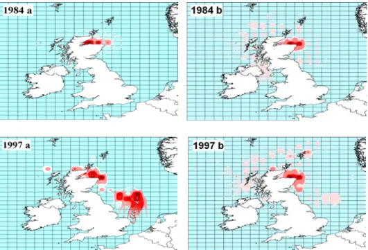
Due to high commercial value, discarding of even small catches of Loligo is thought to be minimal (Young et al., 2004) therefore landings can be assumed to accurately reflect catches. Catch per unit effort (CPUE) is frequently used as an abundance index (Pierce et al., 1994a, 1998; Portela et al., 2005; Wang et al., 2007) however, this study used landings as abundance index rather than LPUE. Since 1998, FRS Marine Laboratory considers effort values of this fishery to be poorly reported due to a change in the recording system (Pierce GJ. Pers Com. 2007), but considers landings data to be reliable. In addition to this, a visual comparison between landings and LPUE values (calculated as hours of effort) was performed in this study with GIS. For years before 1997 this comparison revealed similar patterns in both indices, but years after 1997 that resemblance is not shown. Therefore we
regard landings as an adequate abundance indicator and representative of the fishery (Fig. 2 and Appendix I).
As abundance and distribution of cephalopod stock may fluctuate widely from year to year because each year’s stocks consist mainly of new recruits (Bellido et al., 2001), contour maps where made without a standardized scale from one year to another.
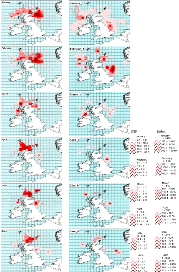
Fig. 2 – Maps showing Loligo forbesi abundance distribution in October of 1984 and 1997, in Scottish waters, achieved from CPUE (a) and landings (b). Squid abundance is characterized by a gradient colour scheme, from higher abundance in dark red to the lower abundance in light pink. (Landings in Kg and CPUE in Kg per hour of effort).
2.1.b. FRS Marine Laboratory performs regularly surveys in Scottish waters with the
purpose to estimate young fish abundance. Although squid are not the target of these surveys, they are thought to be reliably recorded when present. The patchy occurrence of squid records in the survey data is thought to indicate a patchy distribution. The mantle length is one characteristic measured on board.
Length–frequency analysis has been used in several studies, either to establish geographic and temporal patterns (Hatfield and Cadrin, 2001; Arkhipkin et al., 2006) or to resolve the presence of multiple cohorts and give indications of population growth in loliginid squid, including L. forbesi (Hatfield, 1996; Pierce et al., 1994b; Collins et al., 1995b, 1999).
analysis. For that, and according to the months with at least one sample in all years in the respective area, a time series, with data from August from the North Sea (NS) – November/December from the West Coast (WC) – January/February (NS) – March (WC), was built for each year and this order. Series between 1993-1994 and 1995-1996 were not performed due to lack of sufficient data in all months. The mantle length was split into classes: animals between 1-4.5cm were considered to belong to length class 1, between 5-9.5cm to length class 2, 10-14cm to length class 3, 15-19cm to length class 4, 20-24.5cm to length class 5, 25-29cm to length class 6, 30-34cm to length class 7, 35-44cm to length class 8 and squids with 45-73cm were considered to belong to length class 9, in order to simplify the visual analysis.
These series were selected, as in the previous section, because the most important recruitment season is thought to be between months July and November (Collins et al., 1997) and these squid disappear from the fished population by June of the following year (Pierce et al., 1994a; Boyle et al., 1995). In addition other reasons were accounted such as these were the months with at least one sample in all years, because the separation in years allowed a separation of different vessels/gears used in sampling, reducing the bias, and finally because in loliginid squid, size and maturity are positively related (Pierce et al., 2005; Wood, 2000).
2.2. Inshore/Offshore migrations
Collins et al., (1997, 1999), Zuur and Pierce (2004) and Pierce et al. (2005) suggested the existence of two breeding populations and two distinct recruitment peaks of L. forbesi, in Scottish and Irish waters. However is not clear from which cohort the two recruitment periods are derived. Therefore this section of the present work intended help to understand, not only the inshore and offshore movements, but also the connection between these movements and L. forbesi life cycle.
2.2.a. To explore the distribution patterns of L. forbesi in relation to shore, the distance of
the centre of each ICES subdivision to the nearest coastal point (distance to coast.) was measured in GIS (ArcView 3.3). The nearest point to coast was measured instead of the nearest point to the mainland because it is thought that depth may have a positive influence on squid distribution and the many islands and Scandinavia peninsula, if neglected, could introduce an error.
Because in Scotland, each reported haul is associated with the approximate geographic coordinates where the haul was performed, was possible to combine this information with the measured distance from the centre of each ICES square, and determine the squid abundance distribution relative to coast. To investigate this distribution and eventual inshore/offshore movements, the sum of monthly landings (kg), from each ICES square, was plotted against the distance of the centre of each ICES square to the nearest coastal point, in which the haul was performed. As in GIS analysis section, the distribution series began in July due to the beginning of recruitment season (Collins et al., 1997), and finished in June of the following year, when squid seem to disappear from fishing area (Pierce et al., 1994a; Boyle et al., 1995). These analyses were constructed for all the years in which data from commercial fisheries were available.
2.2.b. In other squid species, such as L. pealeii (Hatfield and Cadrin, 2001) length
frequency analyses have been performed in survey data to study the connection between inshore and offshore movements, and between these movements and the life cycle. In the present study, a frequency analysis relating the distance of the haul to coast with L. forbesi length class, was therefore accomplished for each month and each year. The data came from survey vessels but only three classes, representative of small, medium and big squid, were examined, class 2 (5-9,5cm), 4 (15-19cm) and 6 (25-29cm), as size and maturity, in loliginid squid, are positively related (Pierce et al., 2005; Wood, 2000). For that, the number of animals of each length class caught in a ICES square was plotted against the distance of the centre of that ICES square to the nearest coastal point. The series belonging to years 1987-90 and 1994-1996 were not built due to lack of consistent data throughout the months. As in length-frequency analysis, annual series were created with data from August (NS) - November/December (WC) – January/February (NS) – March (WC), because these were the months and areas with at least one sample in all years and because one of the hypothesis is that L. forbesi recruitment season begins in July, and finishes in June of the following year (Collins et al., 1997).
2.3. Environmental analysis and statistics
using an identity link function (i.e. Gaussian) was used as Hastie and Tibshirani (1990) and Zuur et al. (2007) suggested for non-linear data. However, the GAM approach does not take into account the auto-correlation of the different variables and also of these variables with years, due to the structure of data where years had to be combined. Additionally, the residuals dispersion showed great trend and the degrees of freedom of the model were extremely high which revealed that this approach was not appropriate (see Appendix II). GAM was therefore extended to a generalised additive mixed model (GAMM) as Lin and Zhang (1999) proposed for analysis of correlated data, where normally distributed random effects are used to account for correlation in the data.
To fit the model, the GAMM function available from R (version 2.4.0) mgcv library was used. The model selection was based on the absence of trend in residuals, and on identifying which explanatory variables had significant effects (significance is accepted only if p<0.001) with low degrees of freedom. The difference in the number of observations between data sets provided a reason to neglect the value of Akaike Information Criterion (AIC) for selection of the best fitted model, however was took into account if disproportionably high because can indicate the model is not well fitted to data.
SST was downloaded from the NCAR (National Center for Atmospheric Research, USA) web site, with a spatial resolution of 1o longitude by 1o latitude therefore had to be re-sampled to the spatial resolution of 1o longitude by 0.5o latitude, the same as the ICES statistical rectangles. This data are monthly average model results from remotely sensed data, survey temperature data, and sea ice distribution, (Reynolds and Smith, 1994). Sea depth data were downloaded from the website of the National Geographical Data Center, National Oceanic and Atmospheric Administration (NOAA, USA). The original data is gridded data with 5o by 5o resolution, therefore the mean depth of single ICES rectangle was calculated.
2.3.a. To model Loligo forbesi size distribution, the research survey data were divided into
seasons: autumn/early winter (November and December), winter (January and February), spring (March and April) and summer (June to October). Each season had all years combined because available data are very variable from one year or season, to another; hence in some years observations are very few which could decrease the model strength. Therefore to minimize year impact on the model, this parameter was introduced in the
in selecting the best model, two data sets were built for each season. The first incorporated each length class of each haul as a sample (response variable), and the second the average length of squid caught in each haul. A third option, each squid caught as an independent sample, was discarded because not only could introduce an error due to pseudo-replication (each squid is not a truly independent sample), but also because results showed similar patterns to those for the other two data sets, even not taking into account frequency of squid in each haul (see appendix I for more details) and as a final reason because the number of observations became to big to run in R which would lead to the introduction of one more difference in methods. Therefore for final result, a comparison between the models from each dataset was executed. GAMM was fitted to length (response variable, cm) with distance to coast of the centre of the ICES square sampled measured in miles, depth (m) and sea surface temperature (SST, oC) at which haul was performed, as explanatory variables.
2.3.b. As a final approach of this thesis, an attempt to find the relationships between squid
abundance and environmental conditions was carried out in fishery data. However, one characteristic of L. forbesi fishery is that is mostly by-catch (Pierce et al., 1994a; Pierce and Boyle, 2003; Chen et al., 2006; Young et al., 2006a) and therefore a large number of zero landings per haul is common. Due to the reasons explained above in this section, the approach to find links between environmental conditions and veined squid, was the application of a GAMM, however when modelling fishery data, residuals distribution was a problem revealing a very specific trend that indicated the model was not appropriate. Therefore, as data distributions with a high proportion of zero values are difficult to model in one step, a presence/absence approach was first considered and only afterwards the distribution of local abundance was modelled but only using presence data, as Maravelias (1999) and Bellido et al. (2001) suggested. To apply a GAMM in these presence data, landings values were natural log transformed, as the range of values was too wide, revealing some very extreme values that were interfering with residuals distribution, although all explanatory variables were kept once their transformation revealed no improvement to the model.
In both models, data from 1985 to 2004 were used because SST is only completely available since then, landings were used as response variable and distance to coast of the
3. Results
3.1. West Coast to North Sea migrations
3.1.a. Loligo forbesi appears to be widely distributed around the Scottish coast. Commercial
hauls were performed all around Scotland but the contour maps from fishery data reveal, in most of the studied years, a spatially restricted peak of abundance off North Scotland around May/June and an increase in abundance, with a spread in spatial distribution, towards the winter season. After this season, abundance begins to decrease and the spatial distribution also contracts. However, the spatial distribution does not show any clear and consistent pattern across all years in the time series, as we can see from the examples given in Fig. 3 and 4, representative of the years 1988-1989 and 2000-2001, respectively (see all annual GIS maps in Appendix III).
GIS maps reveal, in some years, a movement of the centre of abundance of L. forbesi from the West Coast to the North Sea in winter. However in other years, high squid abundance seems to appear mainly on the West Coast or mainly in the North Sea, or even shows a movement towards the West Coast in winter. L. forbesi seems to appear on the West Coast during spring and in the North Sea during summer in some years, but this is also not a consistent pattern, and again high squid abundance during both these seasons can appear on just one coast of Scotland. In some years, two distinct abundance peaks can also be seen in different areas. These maps are therefore geographic evidence against a consistent migration of veined squid migration from the West Coast of Scotland to the North Sea in wintertime and back again to West Coast in spring as previously hypothesised.
3.1.b. The length frequency analysis performed on survey data demonstrates that L. forbesi
length distribution, for the same area and month, is very variable between years (Fig. 5). During August in the North Sea, there is a consistent dominance of small squid, especially length class 2; however, for the remaining seasons, squid size seems to show no clear pattern. In some years, the size classes in November-December are higher than in summer of the same year, and smaller than in January-February of the following year, while changing from West to East coast as expected. However this described pattern is not consistent in all years. In some other years, smaller squid in January-February than in November-December, or equivalent in size, can be observed along the different areas. The occurrence of relatively small squid in winter season, or even a mixture of sizes class is also apparent. When approaching spring in the West Coast, in several of the years for which data
were available, squid seem to be smaller than in the previous season. During winter in North Sea, squid length classes are bigger than in spring on the west coast, in agreement with the present hypothesis; however there are exceptions. In some years, L. forbesi length class in spring is either the same as the previous season or bigger, which is not consistent with the present hypothesis. Length frequency analysis therefore does not provide evidence of veined squid migration from the West Coast of Scotland to the North Sea in wintertime, and back again to West Coast in spring (see Appendix IV).
3.2. Inshore/Offshore migrations
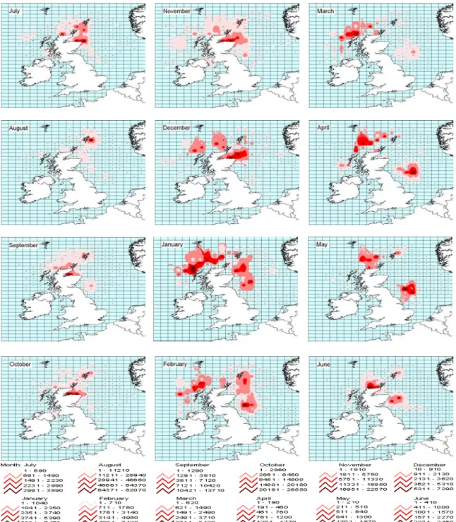
3.2.a. In Scottish waters, L. forbesi appears both inshore and offshore (Fig. 6). Between
May and October, squid are caught mostly inshore since, according to the graphics of the distance to coast of squid abundance, only a very low abundance can occasionally be found in areas distant from the coast. However, between November and April of the following year, squid seem to be appearing both in inshore and offshore grounds. Therefore, around summer and autumn, as we can see from this analysis, L. forbesi tend to be close to shore, and around winter and spring time, they also appear far from the coast but never completely disappear from the inshore grounds. It is also visible that, in some years, the distance to coast of the main centre of squid abundance is slightly variable within months, in that abundance peaks can appear in, or disappear from, offshore grounds one month earlier or later.
Apart from this variation in timing, the appearance of L. forbesi in inshore and offshore grounds is clear and can be described as consistent. However, the movement to offshore grounds and from this area to inshore grounds is not as clear, since squid never really leave inshore areas (see Appendix V).
Fig. 3 – Contour maps of the annual distribution of L. forbesi abundance (Kg), from July of the year 1988 until June of the following year, 1989. Black dots represent the presence of haul(s) in the ICES square.
Fig. 4 – Contour maps of the annual distribution of L. forbesi abundance (Kg), from July of the year 2000 until June of the following year, 2001. Black dots represent the presence of haul(s) in the ICES square.
Fig. 5 – L. forbesi length-frequency distributions from 1988/1989 (left) and 2000/2001 (right). The series starts in August with data from the North Sea (NS) and November-December from the West Coast (WC), and continues to the following year in January-February with data from NS and March from WC. Animals of length class 1: 1-4.5cm; length class 2: 5-9.5cm; length class 3: 10-14cm; length class 4: 15-19cm; length class 5: 20-24.5cm; length class 6: 25-29cm; length class 7: 30-34cm; length class 8: 35-44cm; length class 9: 45-73cm.
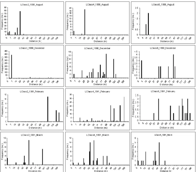
3.2.b. L. forbesi from length classes 2, 4 and 6 seem to appear in both offshore and inshore
grounds. The appearance of some squid in offshore grounds, between November and April, seem to be visible in the analysis of the distance of particular length classes from the coast (Fig. 7). Similar to what is seen in offshore areas, squids appearing exclusively in inshore grounds, around August, belong to all length classes studied in this section.
spring season is approaching they seem to spread to offshore waters, while never disappearing from inshore waters. On the other hand, squid of length class 4 and 6 show a similar pattern, emerging both inshore and offshore all year, but with very low frequency in offshore waters in summer (August). In spring (March) squid seem to be closer to coast than in the previous season. This analysis of size in relation to distance from the coast revealed a spatial pattern throughout the year that is consistent with the above results of the distribution of abundance in relation to coast. These indicate some possible movements to offshore waters in winter and to inshore waters in spring, performed by both small and large squid (see Appendix VI).
3.3. Environmental analysis and statistics
3.3.a. Using a GAMM approach to analyse average squid size for both survey datasets, (A)
treating the frequency of each length class present in each haul as a data point and (B) using the frequency of the average length from each haul respectively, revealed that the distance from coast where a haul is performed is the most significant explanatory variable in most seasons (see Tables I and II, respectively). The exception to this trend is the same in both models: during summer months, depth and SST seem to be the most significant variables, although the smoother for the effect of distance to coast is still significant for model A. When modelling A, all explanatory variables are significant but in B the same is only shown in spring (March-April). In autumn and winter the variable “distance to coast” is the most significant in both models. However when applying the GAMM to A, depth and temperature seem to have significant effects but when modelling B, these parameters seem to lose their effect on squid size distribution (p>0.001). In model B during autumn, even the effect of the smoother distance is very weak. During spring months, for both models A and B, effects of all explanatory variables are significant, but distance to coast is the most important variable in model B and depth is the most important in model A, although with very similar p values.
Regarding the degrees of freedom of the smoothers for these models, these vary between ~1 and ~8 in all seasons and for all explanatory variables. The smooth term “distance to coast” reveals the lowest values in almost all seasons (i.e. the effect is closest to being linear), but there is one exception to this pattern in autumn/early winter months, in which SST seem to
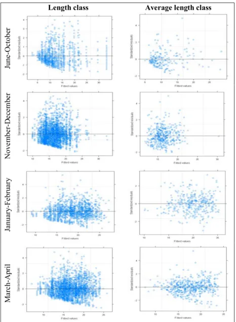
appropriate, since there is no apparent pattern in plots of standardised residuals against the fitted values for the models (Fig. 8).
Fig. 6 – Distance to coast (miles) of L. forbesi abundance for each month of 1990, starting in July and finishing in June of the following year, 1991.
Fig 7. – Distance to coast (miles) of L. forbesi, with length class 2 (left, from 1 to 4.5 cm), 4 (middle, from 15 to 19 cm) and 6 (right, from 25 to 29 cm), occurrence frequency for each month of 1990, starting in July and finishing in June of the following year, 1991.
The analysis of the residual graphics of the models A and B for autumn/early winter reveal some pattern, in that the majority of residuals are situated where the fitted values are lower, but this reflects the distribution of the data rather than a poorly fitted model. Therefore, given the significance values of the smoothers and the “good” residual distribution, it seems that the GAMM approach is appropriate and fits the data.
Table I - Approximate significance values of smooth terms, Akaike Information Criterion (AIC), square R and number of observations used in the GAMM obtained from each length class of each haul as response variable. The GAMM was fitted for 4 seasons, summer (June to October), autumn/early winter (November and December), winter (January and February) and spring (March and April).
Model A
Summer Autumn/Winter Winter Spring
Distance 3.27e-06 2e-16 2e-16 7.66e-15
Depth 2e-16 5.84e-08 4.99e-06 2e-16
p-value SST 2e-16 1.88e-10 6.27e-05 7.65e-09
Distance 2.588 8.062 1.000 1.000 Depth 6.903 5.145 5.689 7.006 Df SST 7.500 1.608 2.862 6.904 Distance 6.031 12.553 128.754 61.135 Depth 19.855 5.754 4.611 10.760 F SST 12.952 12.943 4.864 6.287 AIC 6721.291 22671.19 10144.30 18465.83 R-sq 0.33 0.0291 0.128 0.108 No. observations 1024 3102 1435 2636
Table II - Approximate significance values of smooth terms, Akaike Information Criterion (AIC), square R and number of observations used in the GAMM obtained from the average length class of each haul as response variable. The GAMM was fitted for 4 seasons, summer (June to October), autumn/early winter (November and December), winter (January and February) and spring (March and April).
Model B
Summer Autumn/Winter Winter Spring
Distance 0.069 0.00120 7.26e-12 1.20e-07
Depth 6.61e-06 0.00203 0.0405 4.80e-06
p-values SST 5.45e-07 0.13455 0.1824 2.93e-05
Distance 1.000 3.927 1.000 1.000 Depth 4.313 1.000 3.236 4.928 Df SST 6.433 1.000 1.000 4.562 Distance 3.344 3.283 50.352 28.819 Depth 4.885 9.639 2.124 4.718 F SST 5.687 2,248 1.785 4.200 AIC 1329.231 2873.046 2305.494 3586.650 R-sq 0.325 0.0823 0.15 0.186 n 207 425 354 535
Length class Average length class June -O ct obe r N ov em ber -D ec emb er Ja nua ry -F eb ru ar y M arc h-A pri l
Fig. 8 – GAMM residuals dispersion. Standardized residuals (y-axis) for both datasets, length class and average length class of each haul as a response variable, against the fitted values (x-axis) of the models.
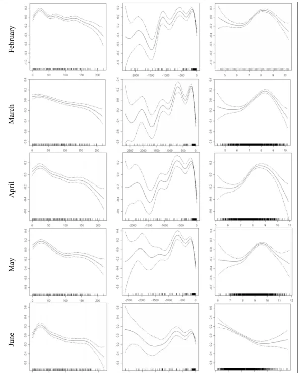
The residual graphics of the two models are shown, in order to compare their goodness of fit. Because these are very similar and because GAMM smooth curves in both models of survey data are also very alike, only the results of model A (Fig.9) are shown in this section as an example (see Appendix VII for model B). GAMM results for all the explanatory variables show smoothing curves with 95% confidence limits. The main trends evident from the smooth curves of the most significant effect in most seasons, distance to coast, reveal a more important effect up to 80 miles from the coast. In winter and spring an inverse relationship seems to exist between length and distance to coast, in that bigger squid tend to
transition between these seasons, in autumn/early winter, distance to coast is in fact the most significant variable but its smoothing curve does not show any clear trend. In general, it seems that the relationship is the same as in summer, however the complex shape of the curve does not allow a clear interpretation.
The effect of depth, in all the seasons, seems to be more important in shallow waters since it is positive in the range between 75 and 250m, with a limit around 150m in autumn and winter. Therefore, below the 250m, depth seem to have no influence in squid size distribution although the wide confidence limits for deeper water may, to some extent, reflect lower data availability rather than the absence of any relationship with depth. Within the limits of positive effect of depth (i.e. in waters <250m deep), size seems to have a relative direct relation with depth, larger sizes in deeper waters. However, this pattern is not consistently seen for depths between 50 and 100m: in spring the opposite trend is apparent and in summer this relationship is linear.
The smoothing curves for sea surface temperature show a more important effect in temperatures above 8ºC. In summer, when temperature is one of the most significant parameters, until 11ºC, smaller squids appear with lower temperatures. However, above ~11ºC this relation inverts, which reveals a peak of size around 11ºC. In autumn small squid also appear in lower temperatures, however in winter, as temperatures are very low, the positive effect is registered only between 8 and 9oC and they seem to prefer the warmer waters. In spring, above 8ºC the relationship between temperature and squid length is apparently linear but again temperatures are very constant and low.
Distance (miles) Depth (m) SST (oC) N ov em ber -D ec emb er Ja nua ry -F eb ru ar y Ma rc h-Ap ri l
Fig. 9 – GAMM results on dataset with each length class of each haul as a response variable. Squid length class is represented as a function of the smooth terms, distance to coast depth and SST for each season. Dashed lines represent two standard error boundaries around the main affects.
3.3.b. When modelling fishery data with a presence/absence approach, effects of all
explanatory variables are equally and highly significant in all months (Table III), with the exception of depth in September and June for which higher p-values were seen, although still very significant (p<0.001). The model also shows very similar degrees of freedom throughout the examined months for all variables, ~1-8, although SST have the lower values, ~1-5, indicating almost linear relationships. This analysis reveals therefore that all studied environmental conditions are important to determine squid presence.
SST and bathymetry. There is one exception to this, for depth in July, August and September that seems to reveal no positive effects due to wide confidence limits. The smooth term for distance to coast indicates an important effect of distance on veined squid presence throughout the fishing area but the trend disappears for hauls farther from the coast, beyond approximately 175 miles. These smooth curves reveal that, in all months, L. forbesi is present until 25 miles from the coast and begins to disappear after this once a peak is seen at this distance. Bathymetry only has a positive, but strong, effect between 0 and 200m depths, where abundance increases with depth. SST smooth curves reveal an optimal temperature peak of abundance around 10oC and from this temperature abundance decreases with the increase of temperature.
When modelling abundance (given presence) data, the results show some similar trends to presence/absence model, but not in all months. With the exception of variable depth in August, October and June and SST in July, all explanatory variables in all months are highly significant, especially distance to coast (Table IV). Apart from depth in June, these reported exceptions are still significant although with higher p-values, near 0.001. The degrees of freedoms of the models, are low between ~1 and 8, and the explanatory variable “distance to coast” demonstrates values of approximately 1 in all months. The significance values of the smooth terms reveal therefore a good fit of the model that is also seen in standardized residual graphics (Fig. 11) since these show no important trends. This analysis reveals that all environmental variables, especially distance to coast, influence L. forbesi abundance in the IVa and b and VIa ICES subdivisions.
GAMM smooth curves of presence data derived from Scottish fisheries (Fig. 12) show very specific patterns and positive effect of the variables throughout the months, in part similar to those found in presence/absence model but quite different, in some months, to those found in when modelling survey data to relate size distribution with environmental conditions. This presence model shows that abundance increases towards the coast in all months and the effect of the smoother begins to be negative from 175 miles from the coast, just as in the presence/absence model, and confidence limits become wider. Depth reveals the most important positive effect on abundance between 0 and 200m and between these values veined squid abundance increases greatly with depth. However, between June and August to October, confidence limits are too wide to reveal any positive. Finally, the SST smoothing curve demonstrates a positive influence of temperatures around 8 and 12oC, allowing for one or two oC of difference according to the season, but as a general pattern,
abundance increases from 7-8oC until ~10oC when it starts to decrease, again as previously seen in the presence/absence model.
Table III - Significance values of smooth terms, Akaike Information Criterion (AIC), square R and number of observations used in the GAMM obtained from presence/absence landings data. GAMM was fitted for all months, from July to June, with all years combined.
P/A Distance Depth SST AIC R-sq n
Jul p=2e-16 Df=8.102 F=16.87 p=2.4e-15 Df=6.791 F=10.06 p=2e-16 Df=4.628 F=28.74 2630.144 0.099 2655 Aug p=2e-16 Df=6.965 F=17.67 p=2.2e-11 Df=3.196 F=9.267 p=2e-16 Df=4.454 F=19.20 2879.897 0.0077 2607 Sep p=2e-16 Df=6.003 F=41.29 p=1.61e-07 Df=1.000 F=27.61 p=2e-16 Df=5.161 F=25.06 2983.174 0.0716 2512 Oct p=2e-16 Df=6.440 F=37.50 p=2e-16 Df=7.552 F=12.17 p=7.03e-15 Df=1.000 F=61.36 2796.13 0.064 2450 Nov p=2e-16 Df=4.151 F=21.665 p=2e-16 Df=8.502 F=24.430 p=7.49e-15 Df=4.749 F=9.789 2575.079 0.116 2502 Dec p=2e-16 Df=7.280 F=11.34 p=2e-16 Df=8.101 F=21.56 p=2e-16 Df=6.351 F=11.13 2053.722 0.123 2249 Jan p=2.24e-15 Df=7.243 F=10.10 p=2e-16 Df=8.491 F=23.70 p=2e-16 Df=4.646 F=10.85 2056.974 0.201 2366 Feb p=2e-16 Df=7.640 F=13.33 p=2e-16 Df=8.429 F=23.27 p=2e-16 Df=5.958 F=22.24 2480.834 0.223 2702 Mar p=3.99e-13 Df=4.008 F=8.788 p=2e-16 Df=8.629 F=36.605 p=2e-16 Df=5.853 F=21.541 2578.621 0.243 2633 Apr p=2e-16 Df=6.137 F=12.41 p=2e-16 Df=8.223 F=27.69 p=2e-16 Df=5.572 F=20.26 2666.174 0.233 2596 May p=2e-16 Df=6.139 F=18.50 p=2e-16 Df=7.993 F=21.55 p=2e-16 Df=5.452 F=16.85 2843.938 0.197 2623 Jun p=2e-16 Df=7.227 F=22.527 p=1.91e-08 Df=6.995 F=6.053 p=2e-16 Df=3.492 F=14.504 2832.598 0.0458 2565
P/A Distance (miles) Depth (m) SST (oC)
Ju
A ugus t Se pt em be r Oc to be r N ove m be r D ece mb er
P/A Distance (miles) Depth (m) SST (oC)
Ja
nua
Fe brua ry Ma rc h A pr il Ma y June
Fig. 10– Landings presence/absence GAMM results. Veined squid landings are represented as a function of the smooth terms, distance to coast depth and SST for each month. Dashed lines represent two standard error boundaries around the main affects.
Table IV - Significance values of smooth terms, Akaike Information Criterion (AIC), square R and number of observations used in the GAMM obtained from presence landings data. GAMM was fitted for all months, from July to June, with all years combined.
Presence Distance Depth SST AIC R-sq n Jul p=2e-16 Df=1.000 F=73.462 p=2.1e-05 Df=5.113 F=4.264 p=0.00017 Df=1.000 F=14.290 2936.355 0.134 712 Aug p=8.72e-06 Df=1.000 F=20.04 p=0.000202 Df=3.198 F=4.09 p=1.86e-05 Df=5.649 F=4.29 3222.792 0.089 781 Sep p=2e-16 Df=1 F=96.14 p=6.68e-06 Df=1 F=20.49 p=2e-16 Df=1 F=73.41 4238.337 0.15 1049 Oct p=2e-16 Df=1 F=360.55 p=0.000269 Df=1 F=13.34 p=2e-16 Df=1 F=163.40 5724.713 0.242 1448 Nov p=2e-16 Df=3.971 F=22.531 p=2e-16 Df=7.730 F=14.432 p=8.4e-15 Df=6.262 F=9.839 6333.957 0.214 1674 Dec p=5.21e-15 Df=1.148 F=23.71 p=2e-16 Df=8.483 F=25.10 p=2e-16 Df=5.062 F=13.18 5920.849 0.19 1593 Jan p=7.1e-16 Df=2.333 F=16.48 p=2e-16 Df=8.524 F=45.78 p=2e-16 Df=4.774 F=14.53 5728.058 0.244 1540 Feb p=1.25e-12 Df=1.000 F=51.34 p=2e-16 Df=8.466 F=26.34 p=3.07e-15 Df=3.710 F=11.06 5179.785 0.2 1418 Mar p=9.29e-12 Df=1.000 F=47.35 p=2e-16 Df=7.983 F=13.40 p=1.68e-11 Df=2.952 F=10.59 4731.185 0.152 1284 Apr p=3.05e-16 Df=1.000 F=68.926 p=2e-16 Df=7.358 F=12.077 p=5.28e-06 Df=3.463 F=5.325 4180.406 0.168 1085 May p=5.53e-13 Df=1.000 F=53.590 p=9.15e-06 Df=5.955 F=4.476 p=2.83e-08 Df=4.397 F=6.052 3746.745 0.121 901 Jun p=1.17e-10 Df=2.995 F=10.010 p=0.00857 Df=2.098 F=3.117 p=5.98e-08 Df=3.391 F=6.879 3208.371 0.094 771
August December April
September January May
October February June
Fig 11 – GAMM residuals dispersion of presence landings data. Standardized residuals (y-axis) plotted against the fitted values (x-axis) of the model for all months.
Ju ly Augus t September October November Decem ber
Fig. 12– GAMM results with using presence landings data. Veined squid landings were log (ln) transformed and are represented as a function of the smooth terms, distance to coast, depth and SST for each month.
Distance (m) Depth (m) SST (oC) Ja nuar y Febr uar y Ma rc h April Ma y June
4. Discussion
4.1. West Coast to North Sea migrations
4.1.a.The spatial distribution of Scottish squid catches broadly reflects the distribution of fishing activity, although very little of this activity is directly targeted at cephalopods (Pierce et al., 2001). Seasonal shifts in the distribution of squid catches are therefore largely due to changes in its distribution and abundance; thus shifts in catch distribution can help to track the recruitment, migration and spawning patterns of the species (Caddy, 1983).
Monthly GIS maps of abundance of Loligo forbesi were the first approach used to verify the first hypothesis, similar to the approach used in a study of the migratory squid Illex argentinus from the southwest Atlantic waters performed by Sacau et al. (2005). Even if abundance and distribution of a cephalopod stock may fluctuate widely from year to year, because each year’s stocks consist mainly of new recruits (Bellido et al., 2001), the analysis of the GIS maps revealed that this species does not routinely migrate from west coast to east coast of Scotland during winter and back to west coast in spring, as previously suggested by Waluda and Pierce (1998). If such movement exists a clear peak of abundance is expected in the West Coast of Scotland during November and December, and around January and February the abundance peak should appear more close to North Sea, the possible spawning area (Waluda and Pierce 1998, Pierce et al., 2001; Young et al., 2006a). During spring, the abundance peak should disappear from North Sea and appear almost exclusively on the West Coast and then move to the North Sea again in autumn to recruit. However, the lack of this pattern in the data analysed during the present study is evidence against such movement.
Two main technical differences were found between Waluda and Pierce (1998) and the present work that could lead to the difference in the results. The fundamental discrepancies are that Waluda and Pierce (1998) used landings per unit effort (LPUE) as an abundance index and mapped data for each ICES rectangle as an isolated abundance point. On the other hand, in the present work, landings are used as abundance index and contour maps were built instead. Both methods have advantages and disadvantages, however the choice of different abundance indexes seems not to change the patterns in the 5 years of common analysis, as predicted after the comparison between these two approaches revealed great similarities, earlier in this work (see methods 3.1.a). It is possible that when using the contour technique to create abundance maps, some values can be omitted because neighbouring abundance values are combined to create the contours. However, abundance
and location of cephalopod populations is highly influenced by the prevalence and scale of their migrations and therefore these migrations involve transfer of hundreds of millions of individuals during phases of high growth (Boyle and Boletzky, 1996), just as dense aggregations are encountered in L. gahi, mainly during the offshore feeding period (Hatfield and des Clers, 1998). These possible omissions are not therefore considered important. When creating maps using each rectangle as isolated point, there is no omission of values however the visual interpretation is significantly more difficult, since the visual gradient is in the size of the abundance symbol and therefore high and low abundance are spatially mixed.
Apart from these difficulties and small differences due to divergent techniques, as briefly mentioned above, the analysis of the small five year series used in Waluda and Pierce (1998) reveals no contradictory results with the present work, since for those few years the patterns are quite similar in both studies. However, when expanding the analysis for twenty years, it is clear that the pattern is not consistent throughout and consequently it is not possible to conclude that Scottish L. forbesi migrate from the West Coast to the North Sea in the winter, and back to west coast in spring, or indeed show any other type of consistent migration pattern. A relative constant pattern in optimal environmental conditions, a fishery tendency once the major directed squid fishery occurs between October and January in Northeast of Scotland (Bellido et al., 2001, Chen et al., 2006), or a possible inflow of squid into Scottish waters from further south, as Pierce and Boyle (2003) suggested for example due to the strong coastal current flow along the West Coast of Scotland that increases nutrient supplies in the area, might be some reasons that led to the apparent migration pattern, described by Waluda and Pierce (1998), in those studied five years. In these years, the major L. forbesi abundance peak in Scottish waters was registered (Zuur and Pierce, 2004), possibly due to the mildest winter climate seen in the North Sea for 50 years (Becker and Pauly, 1996), which could influence squid distribution because, as poikilothermic species, they are affected by water temperature (Pierce et al., 1998; Sims et al., 2001; Bellido et al., 2001).
The GIS maps of veined squid abundance also reveal a spatially restricted peak of abundance to the North of Scotland, around June, followed by a spatial expansion of abundance when approaching the winter season. Although the pattern is not evident in every
site. One final observation of these maps was two distinct abundance peaks, either in different coasts or in the same but one much further south than the other. This can suggest that the two described veined squid cohorts (Collins et al., 1997, 1999; Zuur and Pierce, 2004, Pierce et al., 2005) might have different migratory behaviours as Arkhipkin et al. (2004) discussed for the migratory squid L. gahi. However, these two abundance peaks are not visible in all years and therefore it is not possible to detect any clear pattern. One other possibility is the migration of the English L. forbesi cohort into more northern waters in some years, since Sims et al. (2001) reported that according to environmental condition this species could vary its migration range.
4.1.b. Although the GIS maps seem to be quite consistent in revealing an absence of
migratory movements of L. forbesi from the West Coast of Scotland to the North Sea, or any other consistent movement pattern, some uncertainties regarding the technique applied and the complexity of data might still remain. Therefore in support of the suggestion of non-migratory behaviour, the length frequency analysis performed using survey data revealed a similar result, i.e. that there is no consistent migration pattern from one coast to another as Waluda and Pierce (1998) suggested.
From this analysis, as was expected since summer-autumn is the most important recruitment season, the time series graphics revealed the presence of small to medium-sized animals in August in the North Sea (NS). When approaching November/December on the West coast (WC), squid length is expected to increase, and to continue to increase in January/February (NS), because winter is suggested to be the most important spawning season (Collins et al. (1997). Since size and maturity are positively related (Wood, 2000; Pierce et al., 2001), these breeders should belong to the higher length classes. On the other hand, later on in spring (April), the first wave of recruitment (i.e. smaller animals) is expected to appear on the west coast (Pierce et al., 1994). However this size gradient pattern was not apparent. In August (in the North Sea) most animals present were small (length class 2), but when approaching winter it seems that the growth is not consistent throughout the examined years, and it also seems that in spring the existence of small squids is not regular.
Nevertheless, L. forbesi life cycle is more complex than described above. According to Collins et al. (1997, 1999), Zuur and Pierce (2004) and Pierce et al. (2005), veined squid have two spawning seasons, in winter (around January) and in summer, although the latter is not important as the first. Two recruitment seasons also occur in Scottish waters, the most
exclusively length class 2 (5-9.5cm) in August is evidence of the already described summer recruitment season, future winter spawners (Pierce et al., 2005), because according to Pierce et al. (1994b) full recruitment to the fishery occurs at a mantle length of approximately 15cm. This length frequency analysis can also reinforce the suggestion of a second recruitment season since length class 1 or 2 animals were also present in other seasons. However, there was no other peak of recruitment that was as clearly defined as in autumn, which can also indicate that recruitment season is extended for several months as suggested by Lum-Kong et al. (1992) and Boyle et al. (1995). The existence of two (or more) cohorts (or micro-cohorts) in the same sampling area can however interfere with the length frequency analysis, hiding possible size distribution patterns within cohorts. Other factors can affect with the ease which results of this analysis can be interpreted, such as the possible reduction of female size during spawning season (Collins et al., 1997), the highly variable growth rates - veined squid reveal for example (at least) two sizes at maturity (Pierce et al., 1994, Collins et al., 1999; Smith et al., 2005), and also the incorrect identification of small squid. It has been reported that sometimes the loliginid Allotheutis can be confused with small L. forbesi in fisheries data, since species ID is not confirmed, however in survey samples this identification is confirmed although some errors are suspected to be made (Pierce et al., 2005).
4.2. Inshore/Offshore migrations
4.2.a. Mangold-Wirz (1963) stated that demersal and near-bottom adult squid make their
feeding and spawning migrations over the bottom in offshore–onshore directions and studies of other squid species, such as L. pealeii from the northern United States (Hatfield and Cadrin, 2001) or L. gahi from the SW Atlantic, suggest a movement from their nurseries in shallow inshore waters to feeding offshore grounds in deeper waters (Hatfield and Rodhouse, 1994). The hypothesis of an inshore-offshore migration in Scottish L. forbesi was considered in the present study, analysing monthly distance of centres of abundance to the coast. Between autumn (around August/September) and early winter (around December), higher abundance of squid was expected in offshore waters, as Holme (1974) and Sims et al. (2001) reported for English L. forbesi that migrates to inshore grounds during summer and to offshore grounds when autumn approaches. However, the Scottish
grounds, and between November and April (autumn and winter) they appear in offshore waters, although never completely disappearing from the inshore grounds. In some years, high squid abundance appears in offshore grounds one month earlier or later, but this pattern is revealed to be rather consistent between years.
In Scottish and Irish waters, two breeding populations are reported, that correspond to two distinct recruitment peaks (Collins et al., 1997, 1999; Zuur and Pierce, 2004, Pierce et al., 2005). The main recruitment period, in late summer and the beginning of autumn, can be derived from the winter spawning, and the spring recruitment period from the summer breeder population (Collins et al., 1997; Pierce et al., 2005); therefore the pattern emerging from the present abundance graphics suggests that the summer spawning season takes in inshore waters, as well as autumn recruitment. However, where winter breeders’ spawn and spring recruitment occurs is not clear. Boyle et al. (1995) proposed a less defined life cycle, where individual squid may live 18 months or longer and the spawning season can be extended to several months; in this case squids from winter breeders become the summer spawners of the following year. According to this life cycle, recruitment seasons can also be extended and are not seasonally well defined, although it seems that spring recruitment season is apparently more important than the autumn season. The present study suggests that summer spawning occurs in inshore areas but otherwise the location of recruitment and other spawning sites are unclear.
Arkhipkin and Middleton (2002) discussed a possible interaction between two different species, L gahi and I. argentinus, with distinct migratory behaviours around the Falkland waters, and Agnew et al. (1998) reported that, in L. gahi, a changeover between the two cohorts has been indicated by a decline in the overall maturity status of squid, usually in April–May. Therefore, when one cohort is in offshore areas to feed the other is in inshore waters to spawn and this arrangement changes when the maturity season of the offshore cohort arrives (Arkhipkin et al., 2004). Although genetic studies found that L. forbesi on the continental self of the Northern Europe appears to be one single population (Shaw et al., 1999), two distinct cohorts were identified and evidence of genetic resemblance between immature squid from the two recruitment periods is missing (Zuur and Pierce, 2004). These spatial patterns in landings can therefore reveal different migratory behaviors, while one cohort migrates to offshore grounds around November; the other is resident in inshore areas. This would explain the occurrence of a significant level of abundance near the coast all year around and a very low or zero abundance in offshore grounds, during some seasons. The