Daytime ozone and temperature variations in the mesosphere: a comparison between SABER observations and HAMMONIA model

(1)

ACPD

10, 2005–2029, 2010

Daytime ozone variations

S. Dikty et al.

Title Page

Abstract Introduction

Conclusions References

Tables Figures

◭ ◮

Back Close

Full Screen / Esc

Printer-friendly Version

Interactive Discussion Atmos. Chem. Phys. Discuss., 10, 2005–2029, 2010

www.atmos-chem-phys-discuss.net/10/2005/2010/ © Author(s) 2010. This work is distributed under the Creative Commons Attribution 3.0 License.

Atmospheric Chemistry and Physics Discussions

This discussion paper is/has been under review for the journal Atmospheric Chemistry and Physics (ACP). Please refer to the corresponding final paper in ACP if available.

Daytime ozone and temperature

variations in the mesosphere: a

comparison between SABER

observations and HAMMONIA model

S. Dikty1, H. Schmidt2, M. Weber1, C. von Savigny1, and M. G. Mlynczak3

1

Institute of Environmental Physics, Bremen, Germany 2

Max-Planck-Institute for Meteorology, Hamburg, Germany 3

NASA Langley Research Center, Hampton, VA, USA

Received: 1 December 2009 – Accepted: 20 January 2010 – Published: 29 January 2010

Correspondence to: S. Dikty (dikty@iup.physik.uni-bremen.de)

(2)

ACPD

10, 2005–2029, 2010

S. Dikty et al.

Title Page

Tables Figures

◭ ◮

Back Close

Full Screen / Esc

Interactive Discussion

Abstract

The scope of this paper is to investigate the latest version 1.07 SABER (Sounding of the Atmosphere using Broadband Emission Radiometry) tropical ozone from the 1.27 µm as well as from the 9.6 µm retrieval and temperature data with respect to day-time variations in the upper mesosphere. For a better understanding of the processes 5

involved we compare these daytime variations to the output of the three-dimensional general circulation and chemistry model HAMMONIA (Hamburg Model of the Neutral and Ionized Atmosphere). The results show good agreement for ozone. The ampli-tude of daytime variations is in both cases approximately 60% of the daytime mean. During equinox the daytime maximum ozone abundance is for both, the observations 10

and the model, higher than during solstice, especially above 80 km. We also use the HAMMONIA output of daytime variation patterns of several other different trace gas species, e.g., water vapor and atomic oxygen, to discuss the daytime pattern in ozone. In contrast to ozone, temperature data show little daytime variations between 65 and 90 km and their amplitudes are on the order of less than 1.5%. In addition, SABER 15

and HAMMONIA temperatures show significant differences above 80 km.

1 Introduction

The sun influences the thermal structure, dynamics, and chemistry of the Earth’s mid-dle atmosphere. If ultraviolet (UV) radiation levels alter, midmid-dle atmospheric ozone is e_ffected as well as other trace gases formed by photolysis from a direct radiation e_ffect 20

and due to a dynamical response to solar variability (indirect effect). In particular, the response of ozone above 60 km to variations in UV radiation is not well established. In comparison with the 27-day solar rotation signal (e.g., Chen et al., 1997; Hood and Zhou, 1998; Ruzmaikin et al., 2007; Gruzdev et al., 2009; Dikty et al., 2010) and the 11-year solar cycle response (e.g., Haigh, 2003; Hood, 2004; Crooks and Gray, 2005; 25

(3)

ACPD

10, 2005–2029, 2010

S. Dikty et al.

Title Page

Tables Figures

◭ ◮

Back Close

Full Screen / Esc

Interactive Discussion variation of UV radiation inflicts a by far greater response in mesospheric ozone.

In the following we will refer to “daytime” variations as to (ozone and temperature) variations between sunrise and sunset, i.e. in the tropics between 6 h and 18 h solar local time. The daytime patterns will be the main focus of this paper. The term “diurnal” will be reserved for variations on the 24 h time scale. The amplitude of daytime ozone 5

variations in the upper mesosphere from sunrise to sunset is about 60% of the daytime mean with extreme ozone values between 0.01 to 0.4 ppm at 77.5 km and 0.1 to more than 1 ppm for altitudes 85 km and above.

An early study by Vaughan (1984) summarizes the basics of mesospheric ozone chemistry. He used ozone data from rocket-borne instrumentation and temperature 10

data from SAMS on Nimbus-7 and compared these with the output of a radiative pho-tochemical model. Other early references to mesospheric ozone chemistry are the papers by Allen et al. (1984a,b), wherein they pointed out the significance of oxygen-and hydrogen-containing species oxygen-and the temperature profile on the diurnal variability of ozone. Data used in these papers are from ground-based and rocket borne in-15

strumentation at mid-latitudes. Several other studies investigated diurnal ozone varia-tions in the mesosphere, including nighttime, with satellites (Ricaud et al., 1996; Marsh et al., 2002; Huang et al., 2008a; Smith et al., 2008) and ground-based observations (Connor et al., 1994; Haefele et al., 2008). Ricaud et al. (1996) also compared their observations with model results. Ground-based observations done in the Bordeaux 20

area were compared to a one-dimensional photochemical model by Schneider et al. (2005). They clearly saw a diurnal pattern and a semi-annual oscillation (SAO) signal above 50 km altitude. All of the above mentioned studies show that with nightfall the photo-destruction of ozone stops and ozone quickly reaches a high nighttime equilib-rium in the mesosphere. The models used by Ricaud et al. (1996) and Sinnhuber et al. 25

(2003) did not show any variations during night, and observations showed little to no variations.

(4)

ACPD

10, 2005–2029, 2010

S. Dikty et al.

Title Page

Tables Figures

◭ ◮

Back Close

Full Screen / Esc

Interactive Discussion in the altitude range between 70 and 95 km. They attributed the increase in ozone in

the afternoon in the upper mesosphere to the migrating diurnal tide. Air that is rich in atomic oxygen is believed to be pumped down from the lower thermosphere and to form ozone on recombination with molecular oxygen. SABER temperature data have been used, e.g., by Zhang et al. (2006) and Mukhtarov et al. (2009) to study tidal signatures 5

between 20 and 120 km altitude within ±50◦ latitude. The solar diurnal tide has also

been investigated by Achatz et al. (2008) who utilized a combination of HAMMONIA and a linear model.

Smith et al. (2008) were recently reporting on high ozone values at the nighttime mesopause observed in SABER version 1.07 ozone derived from 9.6 µm radiance. 10

They used a simplified model of the diurnal migrating tide to show that the high night-time ozone values (up to 40 ppm) are a result of an upward motion of air low in atomic hydrogen and atomic oxygen combined with low temperatures, as a result of adiabatic cooling.

The paper by Huang et al. (2008a) can be seen as a precursor to the present study. 15

They reported on SABER version 1.06 diurnal ozone variations (derived from 9.6 µm radiance) over 24 h with the help of a two-dimensional Fourier least squares analysis. They were able to determine the diurnal variation as a function of latitude (up to 48◦), altitude and day of year. The analysis was however limited to at least one year of data. Beig et al. (2008) gave an overview of the temperature response to solar activity 20

in the mesosphere and lower thermosphere. They assumed that the temperature re-sponse to solar activity is mainly due to the vertical distribution of chemically active gases near the mesopause and due to changes in the UV radiation.

In this study we use version 1.07 SABER ozone and temperature vertical profiles from 2003 to 2006 to derive daytime variations in the tropical upper mesosphere and 25

(5)

re-ACPD

10, 2005–2029, 2010

S. Dikty et al.

Title Page

Tables Figures

◭ ◮

Back Close

Full Screen / Esc

Interactive Discussion trieval was improved by reducing the physical quenching rates of the ozone vibrational

levels by a factor of 3. In addition to Huang et al. (2008a), we also include SABER temperature data in our analysis and discuss our results with respect to the chemistry responsible for the daytime pattern from HAMMONIA ozone, temperature, and other trace gases. In Sect. 2 we will first summarize the data sources before we will briefly 5

explain in Sect. 3 the methods used to extract the daytime pattern in ozone and tem-perature. The presentation of the results (Sect. 4) and their discussion in Sect. 5 is followed by a summary in Sect. 6.

2 Data sources

2.1 SABER satellite data

10

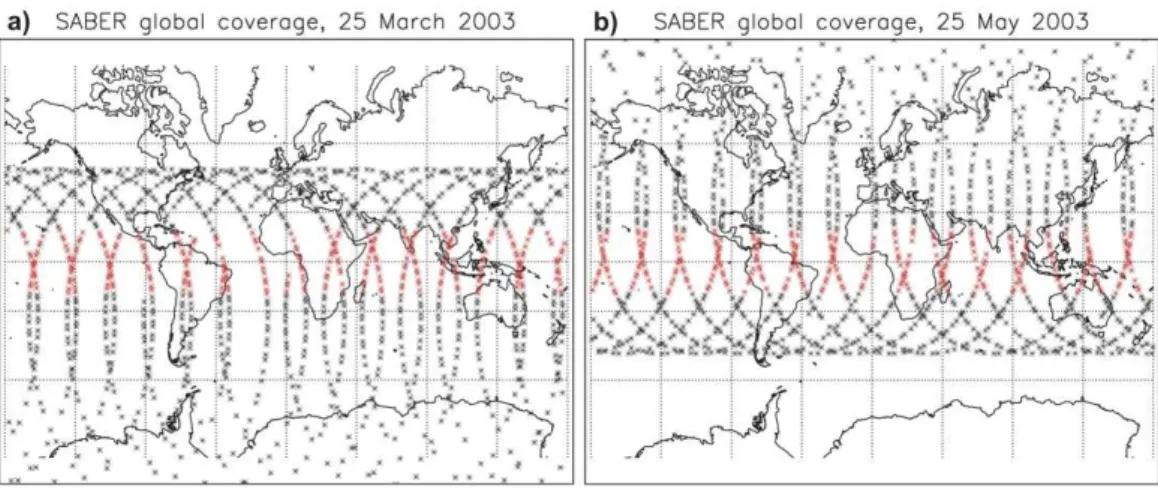
The TIMED (Thermosphere, Ionosphere, Mesosphere, Energetics and Dynamics) satellite has been launched on 12 July, 2001 (Russel III et al., 1999; Remsberg et al., 2008). It circulates the Earth in a low orbit of 628 km mean altitude with an inclination of 74◦. The TIMED satellite is in a non-sun synchronous or drifting orbit with a mean or-bital time of 97 min. Each day the equator crossing time shifts by approximately 12 min. 15

The scanning direction of the SABER instrument is perpendicular to the flight direction of TIMED. Once approximately every 60 days, the TIMED satellite performs a yaw ma-neuver reversing the scanning direction of SABER by 180◦. This measuring geometry limits the latitudinal coverage to 83◦_{S to 52}◦_{N and 52}◦_{S to 83}◦_{N, respectively.}

Con-tinuous time series for high latitudes are therefore not available. Figure 1 shows the 20

spatial coverage for one day of SABER measurements on 25 March, 2003, pointing south and on 25 May, 2003, pointing north. The overall yield is roughly 40 000 profiles per month as SABER solely performs limb measurements.

SABER on board TIMED is an infrared spectrometer measuring limb emission with a spectral range from 1.27 µm to 16.9 µm. The time required to make one “up” or “down” 25

(6)

ACPD

10, 2005–2029, 2010

S. Dikty et al.

Title Page

Tables Figures

◭ ◮

Back Close

Full Screen / Esc

Interactive Discussion 400 km in altitude, although the only channel that measures above 180 km tangent

height is the NO channel at 5.3 µm. The vertical resolution is approximately 2 km and the instrument has a vertical sampling of 0.4 km.

Depending on wavelength (320 nm< λ <_{1180 nm) the photochemical destruction of} ozone can lead to molecular oxygen in its ground state (Eq. 1), at wavelengths short-5

ward of 320 nm, and to oxygen in its first exited state (Eq. 2). The de-excitation leads to airglow emissions at 1.27 µm (Eq. 3) which can be detected by SABER and other spectrometers in orbit, e.g., SCIAMACHY aboard ENVISAT (Bovensmann et al., 1999) and OSIRIS on Odin (Llewellyn et al., 2004):

O3+hν(λ >320 nm) → O2(3Σ)+O(3P) (1)

10

O₃+hν₍λ <_320nm) _→ _O₂₍1_∆₎₊_O(1_D) ₍₂₎

O2(1∆) → O2(3Σ)+hν(1.27 µm) (3)

Many parameters related to the odd-oxygen photochemistry and the energy budget of the mesosphere can be derived from these measurements and are used to infer ozone from the 1.27 µm airglow as described in Mlynczak et al. (2007).

15

In addition to the retrieval of ozone at 1.27 µm that is limited to daytime, the thermal emissions of ozone at 9.6 µm from vibration-rotational energy release can be detected by SABER as described in Rong et al. (2008). The retrieval in the 9.6 µm region per-mits measurements of ozone not only during daylight but at night as well and the ver-tical coverage is not limited to the mesosphere and lower thermosphere. Huang et al. 20

(2008a) studied diurnal variations of ozone retrieved at 9.6 µm. Differences to Huang et al. (2008a) will be highlighted throughout this study. One of which is the emphasis on the daytime (06:00 h–18:00 h solar local time) ozone pattern, in addition to com-parisons to the HAMMONIA model. In this paper we will use ozone data retrieved at 1.27 µm and at 9.6 µm, and we also include temperature data available from SABER. 25

The temperature is retrieved using the spectral information from the two CO2channels

(7)

ACPD

10, 2005–2029, 2010

S. Dikty et al.

Title Page

Tables Figures

◭ ◮

Back Close

Full Screen / Esc

2.2 HAMMONIA model output

In this study we use the output from the three-dimensional general circulation and chemistry model HAMMONIA (Schmidt et al., 2006) to compare to SABER obser-vations. HAMMONIA treats atmospheric dynamics, radiation and chemistry interac-tively. It was developed as an extension of the atmospheric general circulation model 5

MAECHAM5 (Giorgetta et al., 2006; Manzini et al., 2006) and additionally accounts for radiative and dynamical processes in the upper atmosphere. HAMMONIA includes 153 gas phase reactions and 48 chemical compounds. It is a spectral model with (in the current configuration) triangular truncation at wave number 31 (T31) and with 67 levels between the surface and 1.7×10−7hPa (≈250 km). The model includes a full

10

dynamic and radiative coupling with the MOZART3 chemical module (Kinnison et al., 2007). In addition, it accounts for solar heating in the ultraviolet and extreme ultraviolet wavelength regime, a non-LTE radiative scheme, energy deposition and eddy di_ffusion generated by gravity wave breaking, vertical molecular diffusion and conduction, and a simple parameterization of electromagnetic forces in the thermosphere. The process-15

ing of the model output is described in Sect. 3.

3 Data analysis

3.1 SABER ozone and temperature data processing

The SABER ozone profiles retrieved from the 1.27 µm and 9.6 µm radiometer mea-surements as well as temperature profiles were interpolated to a regular height grid 20

(8)

ACPD

10, 2005–2029, 2010

S. Dikty et al.

Title Page

Tables Figures

◭ ◮

Back Close

Full Screen / Esc

Interactive Discussion being outside the 3σ _{value of the whole time series. Small data gaps were closed by}

the use of a spline interpolation. Fortunately, there were no large data gaps from 2003 to 2006.

All daytime time series have a strong signal with a periodicity of approximately 60 days which corresponds to the drift of measurements with local time and the yaw 5

maneuver TIMED is performing. In the tropics this drift in local time is plotted in Fig. 2 for 2003. Yaw maneuvers are indicated as vertical dotted lines. Each dot in the plot represents a single profile and the red solid line indicates the mean local time of mea-surement. The fairly small spread of about half an hour gives us the uncertainty with which we determine the mean local time. The variability of the solar local time of ap-10

proximately half an hour on a given day is mainly due to the fact that the solar local time is slightly different at each latitude in the tropics (movement of the satellite). So by reassigning each day’s area weighted zonal mean profile to its mean local time of measurement (with an error of approximately 30 min around the mean) the analysis of daytime variations becomes possible. The daytime variation is derived from data 15

covering 60 days of measurements between yaw maneuvers. Due to the properties of the TIMED orbit measurements between 11:00 h and 13:00 h solar local time are not possible.

The resulting daytime variation of ozone is shown in Fig. 3 at heights of 69.5, 74.5, 79.5, 84, and 88.5 km (dots) in units of volume mixing ratio. The daytime variations of 20

ozone are also shown in Figs. 4 and 5 (color coding). Here the variation is given as deviation from the daytime (6 h to 18 h) mean in % for pressure levels between 0.1 to 0.001 hPa. SABER temperature anomalies can be seen in Fig. 6 (color coding).

3.2 HAMMONIA model output processing

The HAMMONIA model output used in this study is a 20 year-average from a time-25

(9)

ACPD

10, 2005–2029, 2010

S. Dikty et al.

Title Page

Tables Figures

◭ ◮

Back Close

Full Screen / Esc

Interactive Discussion HAMMONIA ranging from the surface to 1.7×10−7hPa (≈250 km). The vertical

resolu-tion in the mesosphere is about 3 km. Along longitude circles all solar local times are covered, which makes it possible to derive diurnal and daytime variations. As the 3-D model output is available each 3 h, results presented here for specific local times are calculated as an average of 8 locations spaced by 45 degrees of longitude. All latitude 5

steps between 20◦S and 20◦N were chosen to derive an area weighted meridional mean profile. Sunrise and sunset were identified by the sharp decrease and increase in ozone at 0.01 hPa, respectively, at the equator and defined as 6 h and 18 h solar local time, accordingly. HAMMONIA ozone and temperature daytime variations are shown in Figs. 4, 5 and 6 along with SABER ozone and temperature observations. Figure 7 10

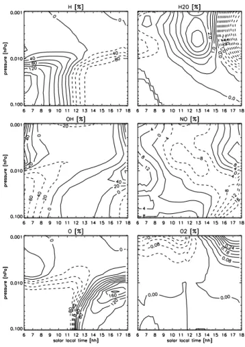
shows model results for atomic hydrogen, water vapor, hydroxyl, nitric oxide, atomic oxygen, and molecular oxygen in terms of a relative deviation from the daytime mean in %.

4 Results

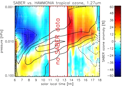
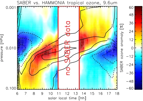
As can be seen in Figs. 4 and 5, SABER and HAMMONIA ozone have distinct and very 15

similar patterns of daytime variation between 0.1 and 0.001 hPa. SABER ozone results are color coded and the HAMMONIA model results are drawn with line contours. While Fig. 4 shows the results for ozone retrieved at 9.6 µm, Fig. 5 shows the results for ozone retrieved at 1.27 µm. For both retrievals and model output, ozone variation from sunrise to sunset can be up to 60% from the daytime mean value. Both observation and model 20

have in common that below about 0.01 hPa ozone values peak in the morning and decrease towards the afternoon. This peak shifts towards the afternoon with increasing altitude.

SABER and HAMMONIA ozone show good agreement in the daytime pattern as shown in Figs. 4, 5 and 8. The maximum daytime peak anomaly observed at 0.05 hPa 25

(≈70 km) in the morning shifts its altitude to about 0.007 hPa (≈80 km) in the

(10)

ACPD

10, 2005–2029, 2010

S. Dikty et al.

Title Page

Tables Figures

◭ ◮

Back Close

Full Screen / Esc

Interactive Discussion anomaly reaches a maximum of 40–50% of the daytime mean, which is higher than

HAMMONIA (30–40%). Negative anomalies are observed in the early morning hours at 0.007 hPa and in the late afternoon near 0.015 hPa in quite good agreement with the model (Fig. 4). In contrast the 1.27 µm retrieval (Fig. 5) does not show this nega-tive anomaly, which could be a SABER retrieval artifact due to twilight conditions. The 5

positive anomaly in the morning hours is also much weaker for the 1.27 µm retrieval (≈10%) than for the 9.6 µm (≈40%). Generally the agreement with the model is better

for the thermal infrared retrieval.

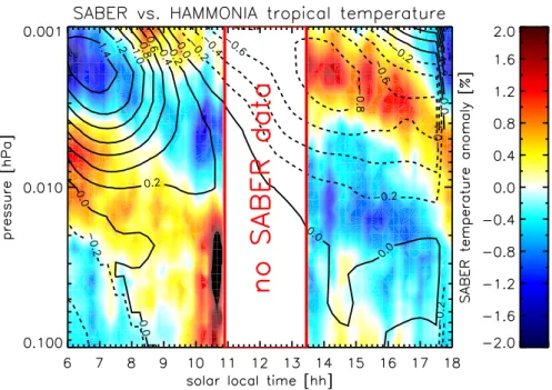
In the case of temperature, the daytime behavior of SABER and HAMMONIA is out of phase for pressure levels above 0.01 hPa (Fig. 6). SABER observes low temperatures 10

in the morning and high values in the afternoon, whereas HAMMONIA predicts high values in the morning and low temperatures in the afternoon. Below 0.01 hPa the agreement is better, yet HAMMONIA does not predict the spurious peak just before the SABER data gap at noon. This might be an artifact in the observations due to averaging effects close to the data gap around noon.

15

The daytime ozone variations depend on the season as is shown in Fig. 3. Especially in the afternoon and above 80 km, ozone reaches up to about 1 ppm in March, April, and May and again in September, October, and November, close to the equinox with increased solar input into the mesosphere. A similar seasonal dependence (albeit with weaker amplitude at high altitudes) is also produced by the HAMMONIA model. 20

Another point is that the ozone minima in the morning do not occur at the same time at 79.5 and 74.5 km. SABER observes the minimum approximately 30–60 min later than HAMMONIA.

5 Discussion

As for the version 1.06 SABER ozone data retrieved at 9.6 µm, Huang et al. (2008a) 25

(11)

ACPD

10, 2005–2029, 2010

S. Dikty et al.

Title Page

Tables Figures

◭ ◮

Back Close

Full Screen / Esc

Interactive Discussion Fourier series with at least one year of data. With the coefficients from the least squares

fit the diurnal variations can be calculated. So, the method is di_fferent but the daytime patterns of Huang et al. (2008a) and ours are qualitatively in agreement. The main distinction of our method is the focus on daytime rather than diurnal variations, whereas Huang et al. (2008a) concentrated on the ozone shifts at daybreak and nightfall. 5

The seasonal variation in ozone that can be seen in Fig. 3 is likely due to the variation of the angle of the incident light. At equinox the sun has the shortest path through the atmosphere in the tropics and thus the strongest potential to photo-dissociate molecu-lar oxygen. At solstice these light paths are slightly longer in the tropics. Huang et al. (2008b) saw large amplitudes in the temperature semi-annual oscillation (SAO) at 75 10

and again at 85 km with a distinct minimum in between, and small SAO amplitudes be-low 80 km, above rising to peak at 95 km. So, a temperature dependency of the ozone SAO in the lower thermosphere cannot be ruled out.

We have shown the good agreement between the SABER and HAMMONIA daytime ozone pattern. In the following, we discuss this pattern with the help of other simulated 15

species (e.g., H, O and OH). Ricaud et al. (1996) explain rising ozone values below 0.01 hPa in the morning with the increased photo-dissociation of O₂and consequently with a higher production of O3due to the high abundance of O radicals. Figure 7 shows

the daytime pattern of O radicals between 0.1 and 0.001 hPa (i.e., 65 to 95 km) as seen by HAMMONIA. The amplitude rises as high as 160% from the daytime mean in the af-20

ternoon slightly below 0.01 hPa, where HAMMONIA ozone reaches its minimum. The decrease of ozone towards the afternoon below approximately 0.01 hPa is assumed by Ricaud et al. (1996) to have its origin in the HO_x catalytic cycles and the net destruc-tion of ozone. HAMMONIA results of the daytime pattern show increasing values of OH and decreasing levels of atomic hydrogen below 0.01 hPa towards the afternoon 25

(Fig. 7). Above 0.01 hPa other mechanisms must be of importance because the O and H radical abundances show almost no daytime pattern. Although we see daytime patterns in H2O and O2, the amplitude is rather small compared to O, OH and H. Also

(12)

ACPD

10, 2005–2029, 2010

S. Dikty et al.

Title Page

Tables Figures

◭ ◮

Back Close

Full Screen / Esc

Interactive Discussion that does not have different amplitudes below and above 0.01 hPa, which indicates that

for the mechanisms involved no distinction can be made between both altitude regions. According to Marsh et al. (2002), the shift of the ozone maximum towards late after-noon with increasing altitude, is accounted for by the temperature (altitude) dependent production rate of HO_x and the associated ozone loss. Notice that there is a sharp 5

edge towards low values in the observational data below 0.01 hPa (≈80 km) and some

data are scattered to higher volume mixing ratios (Fig. 8). This lower boundary may be attributed to an upper limit in H₂O abundances around 75–80 km. An anti-correlation at these heights between O3and HOxhas been concluded by Marsh et al. (2003) after

having investigated data from the Halogen Occultation Experiment (HALOE). 10

Marsh et al. (2002) suggested that the solar diurnal tide “pumps” down atomic oxy-gen for the ozone production in the afternoon (>_{85 km). It is interesting to note that} the daytime variation of ozone is well reproduced by HAMMONIA in contrast to the temperature that is not. This may indicate that chemistry itself may have a larger impact on the abundance of ozone rather than transport effects involving the lower 15

thermosphere. The model, however, underestimates ozone in the afternoon above approximately 0.01 hPa, so the remaining difference could be attributed to solar tides. The minimum early in the morning is caused by the direct photolysis of ozone before enough molecular oxygen is produced to counteract the ozone destruction. It is also assumed by Marsh et al. (2002) that the rise of ozone in the morning hours is due to 20

tides transporting ozone rich air from below. At 0.01 hPa tropical ozone reaches its minimum. At the end of the day ozone rises to its high nighttime equilibrium shortly after sunset, the photochemistry being shut off.

Concerning tides, it is interesting to note that Achatz et al. (2008) have analyzed solar diurnal tides in HAMMONIA and found in general a good agreement with observed 25

(13)

ACPD

10, 2005–2029, 2010

S. Dikty et al.

Title Page

Tables Figures

◭ ◮

Back Close

Full Screen / Esc

Interactive Discussion The amplitudes for temperatures from SABER observations and HAMMONIA model

are relatively small. They only deviate about 1–1.5% (i.e. 1.2–2 K) from the mean at maximum. It remains to be explained why model and observations show a different sign in the daytime pattern. Despite the general similarity of tidal patterns in HAMMONIA and observations as stated by Achatz et al. (2008), our comparison of temperature data 5

suggests a difference in the vertical wavelength of tides in HAMMONIA and SABER. However, the exact analysis of the tides in HAMMONIA is not subject of this study.

6 Summary

Within this study we have compared SABER measurements and HAMMONIA model simulations of upper mesospheric daytime ozone and temperature variations in the 10

tropics between 20◦S and 20◦N.

HAMMONIA and SABER daytime ozone variations show a qualitatively good agree-ment, particularly for the 9.6 µm retrieval. As the agreement is worse in the case of temperature, this suggests that the daytime ozone variations are mainly driven by (photo)-chemical processes and less influenced by transport. The underestimation 15

of HAMMONIA ozone above 0.01 hPa in the afternoon may be due to tidal amplitudes being too weak and associated weak downward transport of air rich in molecular oxy-gen.

Daytime ozone values above 0.01 hPa are higher close to equinox than close to solstice. Volume mixing ratios can even go as high as 1–1.5 ppm in the afternoon 20

for heights above 85 km. Upcoming SABER version 1.08 data will also include water vapor, which will be helpful to constrain the HOx budget and its influence on daytime

ozone.

Acknowledgements. We thank the SABER science team for providing data used in this study.

This work was funded within the SOLOZON project as part of the German national CAWSES 25

(14)

ACPD

10, 2005–2029, 2010

S. Dikty et al.

Title Page

Tables Figures

◭ ◮

Back Close

Full Screen / Esc

References

Achatz, U., Grieger, N., and Schmidt, H.: Mechanisms controlling the diurnal solar tide: Analysis using a GCM and a linear model, J. Geophys. Res., 113, A08303, doi:10.1029/ 2007JA012967, 2008. 2008, 2016, 2017

Allen, M., Lunine, J., and Yung, Y.: The Vertical Distribution of Ozone in the Mesosphere and 5

Lower Thermosphere, J. Geophys. Res., 89, 4841–4872, 1984a. 2007

Allen, M., Lunine, J., and Yung, Y.: Correction to ’The Vertical Distribution of Ozone in the Meso-sphere and Lower ThermoMeso-sphere’ by M. Allen, J. I. Lunine, and Y. L. Yung, J. Geophys. Res., 89, 11827–11827, 1984b. 2007

Beig, G., Scheer, J., Mlynczak, M. G., and Keckhut, P.: Overview of the temperature response 10

in the mesosphere and lower thermosphere to solar activity, Rev. Geophys., 46, RG3002, doi:10.1029/2007RG000236, 2008. 2008

Bovensmann, H., Burrows, J. P., Buchwitz, M., Frerick, J., No ¨el, S., Rozanov, V. V., Chance, K. V., and Goede, A. P. H.: SCIAMACHY: Mission Objectives and Measurement Modes, J. Atmos. Sci., 56, 127–150, 1999. 2010

15

Chen, L., London, J., and Brasseur, G.: Middle atmospheric ozone and temperature responses to solar irradiance variations over 27-day periods, J. Geophys. Res., 102, 29957–29979, 1997. 2006

Connor, B. J., Siskind, D. E., Tsou, J. J., Parish, A., and Remsberg, E. E.: Ground-based mi-crowave observations of ozone in the upper stratosphere and mesosphere, J. Geophys. Res., 20

99, 16757–16770, 1994. 2007

Crooks, S. A. and Gray, L. J.: Characterization of the 11-Year Solar Cycle Using a Multiple Regression Analysis of the ERA-40 Dataset, J. Climate, 18, 996–1015, 2005. 2006

Dikty, S., Weber, M., von Savigny, C., Rozanov, A., Sonkaew, T., and Burrows, J. P.: Modu-lations of the 27-day solar rotation signal in stratospheric ozone from SCIAMACHY (2003-25

2008), J. Geophys. Res., doi:10.1029/2009JD012379, in press, 2010. 2006

Giorgetta, M. A., Manzini, E., Roeckner, E., Esch, M., and Bengtsson, L.: Climatology and Forcing of the QBO in MAECHAM5, J. Climate, 19, 3882–3901, 2006. 2011

Gruzdev, A. N., Schmidt, H., and Brasseur, G. P.: The effect of the solar rotational irradiance variation on the middle and upper atmosphere calculated by a three-dimensional chemistry-30

(15)

ACPD

10, 2005–2029, 2010

S. Dikty et al.

Title Page

Tables Figures

◭ ◮

Back Close

Full Screen / Esc

Interactive Discussion Haefele, A., Hocke, K., K ¨ampfer, N., Keckhut, P., Marchand, M., Bekki, S., Morel, B.,

Egorova, T., and Rozanov, E.: Diurnal changes in the middle atmospheric H₂O and O₃: Observations in the Alpine region and climate models, J. Geophys. Res., 113(D17), doi: 10.1029/2008JD009892, 2008. 2007

Haigh, J. D.: The effects of solar variability on the Earth’s climate, Phil. Trans. R. Soc. Lond. A, 5

361, 95–111, 2003. 2006

Hood, L. L.: Effects of solar UV variability on the stratosphere, Solar Variability and Its Effects on Climate, Geophys. Monogr., 141, 283–303, 2004. 2006

Hood, L. L. and Zhou, S.: Stratospheric effects of 27-day solar ultraviolet variations: An analysis of UARS MLS ozone and temperature data, J. Geophys. Res., 103, 3629–3638, 1998. 2006 10

Huang, F. T., Mayr, H., Russel III, J. M., Mlynczak, M. G., and Reber, C. A.: Ozone diurnal variations and mean profiles in the mesosphere, lower thermosphere, and stratosphere, based on measurements from SABER on TIMED, J. Geophys. Res., 113, A04307, doi: 10.1029/2007JA012739, 2008a. 2007, 2008, 2009, 2010, 2014, 2015

Huang, F. T., Mayr, H. G., Reber, C. A., Russel III, J. M., Mlynczak, M. G., and Mengel, J. G.: 15

Ozone quasi-biennial oscillations (QBO), semiannual oscillations (SAO), and correlations with temperature in the mesosphere, lower thermosphere, and stratosphere, based on mea-surements from SABER on TIMED and MLS on UARS, J. Geophys. Res., 113, A01316, doi:10.1029/2007JA012634, 2008b. 2015

Kinnison, D. E., Brasseur, G. P., Walters, S., Garcia, R. R., Marsh, D. R., Sassi, F., Harvey, V. L., 20

Randall, C. E., Emmons, L., Lamarque, J. F., Hess, P., Orlando, J. J., Tie, X. X., Randel, W., Pan, L. L., Gettelman, A., Granier, C., Diehl, T., Niemeier, U., and Simmons, A. J.: Sensi-tivity of chemical tracers to meteorological parameters in the MOZART-3 chemical transport model, J. Geophys. Res., 112(D20), doi:10.1029/2006JD007879, 2007. 2011

Llewellyn, E. J., Lloyd, N. D., Degenstein, D. A., Gattinger, R. L., Petelina, S. V., Bourassa, 25

A. E., Wiensz, J. T., Ivanov, E. V., McDade, I. C., Solheim, B. H., McConnell, J. C., Haley, C. S., von Savigny, C., Sioris, C. E., McLinden, C. A., Griffioen, E., Kaminski, J., Evans, W. F. J., Puckrin, E., Strong, K., Wehrle, V., Hum, R. H., Kendall, D. J. W., Matsushita, J., Murtagh, D. P., Brohede, S., Stegman, J., Witt, G., Barnes, G., Payne, W. F., Pich ´e, L., Smith, K., Warshaw, G., Deslauniers, D.-L., Marchand, P., Richardson, E. H., King, R. A., Wevers, 30

(16)

ACPD

10, 2005–2029, 2010

S. Dikty et al.

Title Page

Tables Figures

◭ ◮

Back Close

Full Screen / Esc

Interactive Discussion 422, doi:10.1139/P04-005, 2004. 2010

Manzini, E., Giorgetta, M. A., Esch, M., Kornblueh, L., and Roeckner, E.: Sensitivity of the Northern Winter Stratosphere to Sea Surface Temperature Variations: Ensemble Simula-tions with the MAECHAM5 Model, J. Climate, 19, 3863–3881, 2006. 2011

Marsh, D., Smith, A., and Noble, E.: Mesospheric ozone response to changes in water vapor, 5

J. Geophys. Res., 108(D3), 4109, doi:10.1029/2002JD002705, 2003. 2016

Marsh, D. R., Skinner, W. R., Marshall, A. R., Hays, P. B., Ortland, D. A., and Yee, J.-H.: High Resolution Doppler Imager observations of ozone in the mesosphere and lower thermo-sphere, J. Geophys. Res., 107(D19), 4390, doi:10.1029/2001JD001505, 2002. 2007, 2016 Marsh, D. R., Garcia, R. R., Kinnison, D. E., Boville, B. A., Sassi, F., Solomon, S. C., and 10

Matthes, K.: Modelling the whole atmosphere response to solar cycle changes in radia-tive and geomagnetic forcing, J. Geophys. Res., D23306, 112, doi:10.1029/2006JD008306, 2007. 2006

Mlynczak, M. G., Marshall, B. T., Martin-Torres, F. J., Russel III, J. M., Thompson, R. E., Rems-berg, E. E., and Gordley, L. L.: Sounding of the Atmosphere using Broadband Emission 15

Radiometry observations of daytime mesosphericO₂(1∆) 1.27 µm emission and derivation of ozone, atomic oxygen, and solar and chemical energy deposition rates, J. Geophys. Res., 112, D15306, doi:10.1029/2006JD008355, 2007. 2010

Mukhtarov, P., Pancheva, D., and Andonov, B.: Global structure and seasonal and interannual variability of the migrating diurnal tide seen in the SABER/TIMED temperatures between 20 20

and 120 km, J. Geophys. Res., 114, A02309, doi:10.1029/2008JA013759, 2009. 2008 Remsberg, E. E., Gordley, L. L., Marshall, B. T., Thompson, R. E., Burton, J., Bhatt, P., Harvey,

V. L., Lingenfelser, G., and Natarajan, M.: The Nimbus 7 LIMS version 6 radiance condition-ing and temperature retrieval methods and results, J. Quant. Spectrosc. Ra., 86, 395–424, doi:10.1029/2006JD007339, 2004. 2010

25

Remsberg, E. E., Marshall, B. T., Garcia-Comas, M., Krueger, D., Lingenfelser, G. S., Martin-Torres, J., Mlynczak, M. G., Russel III, J. M., Smith, A. K., Zhao, Y., Brown, C., Gordley, L. L., Lopez-Gonzales, M. J., Lopez-Puertas, M., She, C.-Y., Taylor, M. J., and Thompson, R. E.: Assesment of the quality of the Version 1.07 temperature-versus-pressure profiles of the middle atmosphere from TIMED/SABER, J. Atmos. Res., 113, D17101, doi:10.1029/ 30

2008JD010013, 2008. 2009

(17)

ACPD

10, 2005–2029, 2010

S. Dikty et al.

Title Page

Tables Figures

◭ ◮

Back Close

Full Screen / Esc

Interactive Discussion the UARS microwave limb sounder instrument: Theoretical and ground-based validations,

J. Geophys. Res., 101, 10077–10089, 1996. 2007, 2015

Rong, P. P., Russell III, J. M., Mlynczak, M. G., Remsberg, E. E., Marshall, B. T., Gordley, L. L., and Lopez-Puertas, M.: Validation of TIMED/SABER v1.07 ozone at 9.6 µm in the altitude range 15–70 km, J. Geophys. Res., D04306, 114, doi:10.1029/2008JD010073, 2008. 2010 5

Russel III, J. M., Mlynczak, M. G., Gordley, L. L., Tansock Jr., J. J., and Esplin, R. W.: Overview of the SABER experiment and preliminary calibration results, Proc. SPIE Vol. 3756, doi: 10.1117/12.366382, 1999. 2009

Ruzmaikin, A., Santee, M. L., Schwartz, M. J., Froidevaux, L., and Pickett, H. M.: The 27-day variations in stratospheric ozone and temperature: New MLS data, Geophys. Res. Lett., 34, 10

L02819, doi:10.1029/2006GL02819, 2007. 2006

Schmidt, H., Brasseur, G. P., Charron, M., Manzini, E., Giorgetta, M. A., Diehl, T., Fomichev, V. I., Kinnison, D., Marsh, D., and Walters, S.: The HAMMONIA Chemistry climate model: Sensitivity of the mesopause region to the 11-year solar cycle and CO₂doubling, J. Climate, 19, 3903–3931, 2006. 2011, 2012

15

Schneider, N., Selsis, F., Urban, J., Lezeaux, O., de LaNo ¨e, J., and Ricaud, P.: Seasonal and Diurnal Variations: Observations and Modeling, J. Atmos. Chem., 50, 25–47, 2005. 2007 Sinnhuber, M., Burrows, J. P., Chipperfield, M. P., Jackman, C. H., Kallenrode, M.-B., K ¨unzi,

K. F., and Quack, M.: A model study of the impact of magnetic field structure on atmospheric composition during solar proton events, Geophys. Res. Lett., 30(15), 1818, doi:10.1029/ 20

2003GL017265, 2003. 2007

Smith, A. K., Marsh, D. R., Russel III, J. M., Mlynczak, M. G., Martin-Torres, F. J., and Kyr ¨ol ¨a, E.: Satellite observations of high nightime ozone at the equatorial mesopause, J. Geophys. Res., 113, D17312, doi:10.1029/2008JD010066, 2008. 2007, 2008

Soukharev, B. E. and Hood, L. L.: Solar cycle variation of stratospheric ozone: multiple regres-25

sion analysis of long-term satellite data sets and comparisons with models, J. Geophys. Res., 111, D20314, doi:10.1029/2006JD007107, 2006. 2006

Vaughan, G.: Mesospheric ozone - theory and observation, Q. J. Roy. Meteor. Soc., 110, 239– 260, 1984. 2007

Zhang, X., Forbes, J. M., Hagan, M. E., Russel III, J. M., Palo, S. E., Mertens, C. J., and 30

(18)

ACPD

10, 2005–2029, 2010

S. Dikty et al.

Title Page

Tables Figures

◭ ◮

Back Close

Full Screen / Esc

Fig. 1. Example of daily global coverage of SABER measurements. On 25 March (left panel),

(19)

ACPD

10, 2005–2029, 2010

S. Dikty et al.

Title Page

Tables Figures

◭ ◮

Back Close

Full Screen / Esc

Fig. 2. Distribution of solar local times of SABER measurements between 20◦_{S and 20}◦_{N for}

(20)

ACPD

10, 2005–2029, 2010

S. Dikty et al.

Title Page

Tables Figures

◭ ◮

Back Close

Full Screen / Esc

Fig. 3.SABER (dots) and HAMMONIA (solid lines) daytime ozone (1.27 µm retrieval) variations

(21)

ACPD

10, 2005–2029, 2010

S. Dikty et al.

Title Page

Tables Figures

◭ ◮

Back Close

Full Screen / Esc

Fig. 4. SABER (retrieved at 9.6 µm, color coding) and HAMMONIA (contour lines) daytime

(22)

ACPD

10, 2005–2029, 2010

S. Dikty et al.

Title Page

Tables Figures

◭ ◮

Back Close

Full Screen / Esc

(23)

ACPD

10, 2005–2029, 2010

S. Dikty et al.

Title Page

Tables Figures

◭ ◮

Back Close

Full Screen / Esc

Fig. 6.SABER (color coding) and HAMMONIA (contour lines) daytime temperature variations

(24)

ACPD

10, 2005–2029, 2010

S. Dikty et al.

Title Page

Tables Figures

◭ ◮

Back Close

Full Screen / Esc

Fig. 7.HAMMONIA daytime variations of atomic hydrogen, water vapor (top row, left to right),

(25)

ACPD

10, 2005–2029, 2010

S. Dikty et al.

Title Page

Tables Figures

◭ ◮

Back Close

Full Screen / Esc

Fig. 8.Daytime ozone (1.27 µm retrieval) variations as seen by SABER (dots) and HAMMONIA