HESS Opinions "On forecast (in)consistency in a hydro-meteorological chain: curse or blessing?"

(1)

HESSD

8, 1225–1245, 2011

On forecast (in)consistency in a hydro-meteorological

chain

F. Pappenberger et al.

Title Page

Abstract Introduction

Conclusions References

Tables Figures

◭ ◮

Back Close

Full Screen / Esc

Printer-friendly Version Interactive Discussion

Discussion

P

a

per

|

Dis

cussion

P

a

per

|

Discussion

P

a

per

|

Discussio

n

P

a

per

|

Hydrol. Earth Syst. Sci. Discuss., 8, 1225–1245, 2011 www.hydrol-earth-syst-sci-discuss.net/8/1225/2011/ doi:10.5194/hessd-8-1225-2011

Hydrology and Earth System Sciences Discussions

This discussion paper is/has been under review for the journal Hydrology and Earth System Sciences (HESS). Please refer to the corresponding final paper in HESS if available.

HESS Opinions

“On forecast

(in)consistency in a hydro-meteorological

chain: curse or blessing?”

F. Pappenberger1, H. L. Cloke2, A. Persson1,3,4, and D. Demeritt2

1

European Centre for Medium Range Weather Forecasts, Reading, UK

2

Department of Geography, King’s College London, London, UK

3

UK Met Office, Exeter, UK

4

Swedish Meteorological and Hydrological Institute, Norrk ¨oping, Sweden

Received: 11 January 2011 – Accepted: 17 January 2011 – Published: 26 January 2011 Correspondence to: F. Pappenberger (florian.pappenberger@ecmwf.int)

(2)

HESSD

8, 1225–1245, 2011

chain

Title Page

Tables Figures

◭ ◮

Back Close

Full Screen / Esc

Discussion

P

a

per

|

Dis

cussion

P

a

per

|

Discussion

P

a

per

|

Discussio

n

P

a

per

|

Abstract

Flood forecasting increasingly relies on Numerical Weather Prediction (NWP) forecasts to achieve longer lead times (see Cloke et al., 2009; Cloke and Pappenberger, 2009). One of the key difficulties that is emerging in constructing a decision framework for these flood forecasts is when consecutive forecasts are different, leading to different

5

conclusions regarding the issuing of forecasts, and hence inconsistent. In this opinion paper we explore some of the issues surrounding such forecast inconsistency (also known as “jumpiness”, “turning points”, “continuity” or number of “swings”; Zoster et al., 2009; Mills and Pepper, 1999; Lashley et al., 2008). We begin by defining what forecast inconsistency is; why forecasts might be inconsistent; how we should analyse

10

it; what we should do about it; how we should communicate it and whether it is a totally undesirable property. The property of consistency is increasingly emerging as a hot topic in many forecasting environments (for a limited discussion on NWP inconsistency see Persson, 2011). However, in this opinion paper we restrict the discussion to a hydro-meteorological forecasting chain in which river discharge forecasts are produced

15

using inputs from NWP. In this area of research (in)consistency is receiving recent interest and application (see e.g., Bartholmes et al., 2008; Pappenberger et al., 2011).

1 What is (in)consistency?

Forecast consistency refers to the degree to which two forecasts agree about the mag-nitude, onset, duration, location or spatial extent of a given event. In hydrological

fore-20

casting we are typically interested in comparing the degree of consistency between consecutive forecasts from the same model issued at different times. Though with the emergence of ensemble and grand-ensemble (Pappenberger et al., 2008) techniques, this then means assessing the consistency between forecasts made for the same lo-cation and time for different model set-ups and iterations, though as we discuss below,

25

(3)

HESSD

8, 1225–1245, 2011

chain

Title Page

Tables Figures

◭ ◮

Back Close

Full Screen / Esc

Discussion

P

a

per

|

Dis

cussion

P

a

per

|

Discussion

P

a

per

|

Discussio

n

P

a

per

|

of agreement between two different forecasts made for the same future point in time, forecast inconsistency occurs when sequences of (temporally) consecutive forecasts issued for the same future point develop differently and so exhibit a change in behaviour in some way from one another about their predictions of what is going to happen.

1.1 Deterministic forecasts

5

In Fig. 1 this is illustrated for a (deterministic) forecast showing inconsistency in the magnitude of forecasted peak discharge (for a hypothetical case based on the River Severn, UK). These forecasts are from the same model with the same structure and equations. The figure shows four di_fferent forecasts for station X issued on 24, 25, 26 and 27 March. The dotted line indicates the observations and the solid area

repre-10

sents a warning threshold. The first forecast (i) indicates a slight possibility of a flood on 30 March and has a very clear signal, in terms of threshold exceedance, on the 1st April. Although the next forecast (ii), issued on 25 March, shows the same basic pat-tern of increased flow, peaking, as before, on 1 April, the threshold exceedance signal has disappeared. Forecasted river levels exceed warning levels again in the forecast

15

issued on 26 March (iii), but with a lower possibility of flooding on 30 March, while the forecast (iv) issued on 27 March (iv) again does predict flooding. As is typical for many flood forecasting systems, in our case a flood warning is issued depending on whether (or not) a river discharge is exceeded (see in Fig. 2).

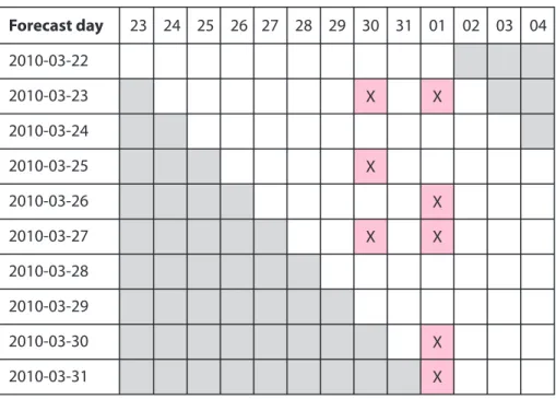
Table 1 shows a typical forecast overview diagram for our hypothetical case. The

20

rows indicate the date and time that the forecast was issued and the columns indicate the date for which the forecast was issued. As the table clearly shows there is incon-sistency between the forecasts, and river discharge threshold exceedance is variously forecast to occur on both 30 March 2010 and 1 April 2010, on either date or neither. Hence inconsistency is demonstrated in the timing of the flood event as well as whether

25

the event happens.

(4)

HESSD

8, 1225–1245, 2011

chain

Title Page

Tables Figures

◭ ◮

Back Close

Full Screen / Esc

Discussion

P

a

per

|

Dis

cussion

P

a

per

|

Discussion

P

a

per

|

Discussio

n

P

a

per

|

is often so apparent because continuous forecasts are translated into binary yes/no threshold exceedence at some time or place in order to issue warnings and calculate skill scores.

1.2 Ensemble flood forecasts

Further complexity is added by the combination of various forecasts into ensemble

5

forecasting systems. Many modern flood forecasting systems rely not only on deter-ministic forecasts, but also on ensemble forecasts (and a combination thereof). In this situation, in addition to the above mentioned definitions, it is necessary to define incon-sistency thresholds based on the number of ensemble members1(either in the form of frequency or probability) over a warning discharge threshold.

10

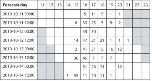
Consider the example of an alert chart from a flood alert system using ensemble weather forecasts as inputs (Table 2). Similar to Table 1 the rows indicate the date and time that the forecast was issued and the columns indicate the date for which the forecast was issued. However, this time the table shows the number of ensembles exceeding a high alert level (for other examples see Thielen et al., 2009a,b). For a

se-15

ries of ensemble forecasts of this sort there are different ways in which it is possible to define (in)consistency between consecutive ensembles (represented by rows in the table) issued at timet_andt₊_1:

1. in terms of the number of ensemble members over the trigger discharge threshold: in this case, the differences for consecutive forecasts range from 0 to 35 between

20

di_fferent forecasts. A di_fference of 35 can be observed between the midnight and noon forecasts issued on the 14. for day 15.

2. the onset of the flood varies between the 14./15. and 16. 1

(5)

HESSD

8, 1225–1245, 2011

chain

Title Page

Tables Figures

◭ ◮

Back Close

Full Screen / Esc

Discussion

P

a

per

|

Dis

cussion

P

a

per

|

Discussion

P

a

per

|

Discussio

n

P

a

per

|

3. the flood lasts from anything between 4 days to 2 days

4. it exhibits a single or double peak.

2 Why are forecasts inconsistent?

Forecast inconsistency comes from various imperfections in the forecasting chain. In medium range NWP the most significant cause of inconsistency are errors in the

spec-5

ification of initial conditions for a non-linear dynamic model so that even with a “perfect” model, meaning a perfect representation of the physics of atmospheric processes (if that can exist) inconsistency is unavoidable. NWP models were more consistent 20– 30 years ago because the poverty of their representations of atmospheric processes and their low spatio-temporal resolutions made them less sensitive to variance in the

10

specification of initial conditions. Thus reducing the quality of the NWP model would improve consistency, but reduce overall skill. At the end of the hydro-meteorological forecasting chain, this inconsistency is complicated by the nonlinear interaction be-tween all imperfections (including initial conditions, forcing, model parameterization, observations etc.; note we assume that every forecast system is always imperfect due

15

to hydrological uncertainty; see Beven, 2006). As a result, the relative importance of di_fferent sources of uncertainty for forecast consistency will depend on exactly which dimension of forecast inconsistency (i.e. the timing or magnitude of the flood peak, its spatial extent or temporal duration) one is concerned with. For example, for typically convective situations flash flood forecasts are usually less consistent than largely

syn-20

optic scale driven floods partially because of the high uncertainties involved in mod-elling convective rainfall location and timing at high resolution (Gupta et al., 2002). Indeed for flash flood forecasts inconsistency about the predicted location of flooding is common, and the tendency is to remain on flood alert while the possibility of a flash flood exists even if the uncertainty about its exact location is high. Inconsistency here

25

(6)

HESSD

8, 1225–1245, 2011

chain

Title Page

Tables Figures

◭ ◮

Back Close

Full Screen / Esc

Discussion

P

a

per

|

Dis

cussion

P

a

per

|

Discussion

P

a

per

|

Discussio

n

P

a

per

|

can have very dramatic effects if there are several flash flood prone areas in the area or if this shift simply means that the rain is falling on the “non flash-flood producing side” of the valley.

The problem of forecast inconsistency is in some way eased through ensemble fore-casting as the ensemble will intrinsically “blend out” individual jumpy forecasts as well

5

as providing a better understanding of initial condition/model uncertainty. However, on the other hand, it makes the conceptual problem of defining in just what sense one set of model runs (individual ensemble members) might be “consistent” with the next more, not less, difficult. Inconsistency exists mainly due to the imperfection of the ac-tual ensemble design e.g. limited number of members and under-dispersivity and thus

10

remains a significant challenge to the forecaster.

3 Quantifying inconsistency

Quantifying inconsistency can be useful but only when it is accompanied by an under-standing of why the inconsistency occurred. Here we make a (unrealistic) binary di-vide between expert users, such as those involved in producing hydro-meteorological

15

forecasts, and non-experts users of hydro-meteorological forecasts among the gen-eral public in order to illustrate extreme positions. We note that in reality there is less differentiation between the groups.

It is important for expert users to find robust ways to identify inconsistency and ex-press it numerically in order to aid their decision making, understand system limitations

20

or compare different forecast systems (assuming that they understand how to interpret the quantification of inconsistency). Examples of evaluation measures include regres-sion, root mean squared error and bias based approaches (Nordhaus, 1987; Clements, 1997; Clements and Taylor, 2001; Mills and Pepper, 1999; Bakhshi et al., 2005) and pseudo-maximum likelihood estimators (Clements and Taylor, 2001). In weather

fore-25

(7)

HESSD

8, 1225–1245, 2011

chain

Title Page

Tables Figures

◭ ◮

Back Close

Full Screen / Esc

Discussion

P

a

per

|

Dis

cussion

P

a

per

|

Discussion

P

a

per

|

Discussio

n

P

a

per

|

et al., 2009) have also been used. Pappenberger et al. (2011) have applied the latter to probabilistic hydro-meteorological forecasts. The number of di_fferent ways in which it is possible to quantify inconsistency introduces its own level of uncertainty to the evaluation, but it remains essential to quantify it in some (or many) numerical ways.

In contrastnon-expert usersmay not necessarily benefit from this information. Users

5

would be able to see for themselves that the forecast has changed. Inconsistency in these circumstances has to be accompanied by an explanation of why it occurs as well as an analysis that is understandable in lay terms. Thus quantification might be based on a verbal (rather than a numerical) basis. This means that one might not use a numerical value for the inconsistency measure, and rather say that scenario A is

10

forecasted, but we expect a possibility of scenario B. This verbal measure would of course be based on a numerically computed evaluation for and by the expert user.

4 Consistency and forecast performance

It could be hypothesised that consistency is an indicator of forecast strength. How-ever we would like to highlight the important fact that, the theoretical basis for this is

15

not necessarily clear cut. Persson and Grazzini (2007) demonstrated that correlation between forecast jumpiness and forecast error (typically 30% according to investiga-tions by see e.g., Ho_ffman and Kalnay, 1983; Dalcher et al., 1988; Palmer and Tibaldi, 1988; Roebber, 1990 and others) is a statistical artefact. Inconsistency and forecast errors are related, but consistency should not be used as a proxy for forecast accuracy

20

(Hamill, 2003), nor does it qualify as a predictor ofa priori skill.

5 The problem of inconsistency

Forecasting preference is usually for consistency. Any forecaster would ideally like to issue a flood warning as early as possible, minimize the error and then update the fore-cast in continuous way. However, hydro-meteorological flood forefore-casts have very high

(8)

HESSD

8, 1225–1245, 2011

chain

Title Page

Tables Figures

◭ ◮

Back Close

Full Screen / Esc

Discussion

P

a

per

|

Dis

cussion

P

a

per

|

Discussion

P

a

per

|

Discussio

n

P

a

per

|

uncertainties not only due to the quality of weather (or maybe radar) forecasts, but also due to the rarity of flood events, which makes it di_fficult to validate model predictions. Flood forecast recipients face similar problems. Unlike daily weather forecasts, which members of the public are accustomed to using and evaluating, flood alerts and other warnings of extreme weather are so rare that there is not the same intuitive feel for how

5

much stock to put in them or how best to respond to uncertain warnings of impending disaster.

One response to the challenge of decision-making in the face of inevitable uncer-tainty about forecast accuracy is to establish a cost-loss function, so as to weigh up the relative costs that would be incurred by taking precautionary action in response to

10

the forecast against the losses that would be incurred if the forecast is ignored and yet proves correct (Murphy, 1977; Richardson, 2000; Roulin, 2007; Laio and Tamea, 2007). However, actually establishing the functional relationship is complex, and the values as-sociated with some costs and losses cannot be easily reduced to monetary ones as is required for a cost-benefit type calculation (Davies and Demeritt, 2000). What value

15

should be put on a life? The question is incalculable, and when the values at stake are sufficiently high (whether in terms of lives and property, dread risk (i.e. nuclear acci-dents or terrorism; cf. Slovic, 1987), or the reputational costs of getting it wrong) then cost/loss functions often go out the window, and pre-emptive action is taken regardless of whether one gives much credence to the likelihood of the forecasted event.

More-20

over hits, misses, false alarms and correct negatives often have significantly different weight from each other in flood forecasting (Demeritt et al., 2010; Ramos et al., 2010) than that that is implied by a standard contingency table (Bartholmes et al., 2009). There is also the key issue that what counts as a meteorologically correct forecast (i.e. rainfall>_{30 mm/h, which is the design capacity for urban drainage) may not result}

25

(9)

HESSD

8, 1225–1245, 2011

chain

Title Page

Tables Figures

◭ ◮

Back Close

Full Screen / Esc

Discussion

P

a

per

|

Dis

cussion

P

a

per

|

Discussion

P

a

per

|

Discussio

n

P

a

per

|

Flood forecasters are well aware of the problem of “crying wolf” and the risk that a sequence of false alarms will result in people no longer taking action and hence increase the costs of a hit (value of losses!). In addition a miss can be catastrophic for the individuals directly affected by the flooding and also for the organisation which failed to alert (Dedieu, 2009). Consideration of reputational damage plays an important

5

role in flood forecasting and consequentially has to be added to the cost, which can be different for different people given the same event. The cumulative effect of these two peculiarities leads to the fact that flood forecasters are very unwilling to change their warning simply based on the latest new forecast (Demeritt et al., 2010; Ramos et al., 2010; Norbert et al., 2010)2. Therefore, reducing the false alarm rate and strong

10

autocorrelation3 between warnings both play a strong role in the design of any flood warning system. But this is just one kind of error: the false positives (type 1) error. There is also the type 2 error of missed events. While EPS helps to increase sensitivity to possible surprise, and so decrease the frequency of type 2 errors, it tends (with low thresholds needed to avoid type 2 errors) to lead to lot of type 1 errors. In the case

15

of the EFAS, lagged forecasts are used to reduce this sort of error, and this temporal consistency, or persistency, of forecasts is then built into the decision making process (Bartholmes et al., 2009): at least three consecutive flood forecasts must predict that a critical discharge threshold will be exceeded for the same river stretch, for a flood alert to be issued. This use of consistency reduces the number of false alarms and at

20

a minimal cost to the hit rate.

This cannot be seen as a general rule as it depends strongly on the individual cost-loss function. It leads to under-forecasting, which may not always be desirable and

2

It may be that that this is synonymous with the pre-NWP model culture that existed in meteorology and it may be that flood forecasters will also eventually adopt the approach of always using the latest forecast the more they get used to meteo-hydrological forecasting chains. On the other hand, hydrological forecasting as such has been performed for many decades and attitudes do not seem to have evolved towards the current culture in meteorology.

3

(10)

HESSD

8, 1225–1245, 2011

chain

Title Page

Tables Figures

◭ ◮

Back Close

Full Screen / Esc

Discussion

P

a

per

|

Dis

cussion

P

a

per

|

Discussion

P

a

per

|

Discussio

n

P

a

per

|

strongly depends on the envisaged lead time. Bartholmes et al. (2009) demonstrate that this is the best solution within the context of the European Flood Alert System. Different uses for forecast consistency may be necessary in other forecasting contexts.

6 The uses of inconsistency

Despite the preference of hydrological forecasters for consistency one should not

ig-5

nore the advantages of inconsistency. Inconsistency discourages the forecaster from relying on the latest forecast, and instead encourages them to seek out alternative in-formation in an ensemble system, previous forecasts or from other models. Persson and Grazzini (2007) argue that a consistent forecast may lull forecasters into a false sense of reliability, which exacerbates difficulties in decision making when sudden

sur-10

prising forecasts arise. In the same way a gradually changing forecast may contribute to a higher sense of reliability than an abruptly changing one (Lashley et al., 2008) and thus the magnitude of inconsistency is of particular importance. Inconsistency can thus be an asset if it alerts forecasters to possible forecast problems and highlights alternative developments (see full details in Persson and Grazzini, 2007).

15

To illustrate these benefits of inconsistency, we refer back to Table 1. It can be clearly seen that a flood event could occur either on 31 March or 1 April. Here we would ar-gue that a warning should be issued at 26 March stating that there is the possibility of a flood between 30 and 1 April. This warning should stay in place until 29 March, when it is changed to the fact that the flood may happen on 1 April. In this way the

20

communicated warning would have a considerable consistency but still allow for the ambiguity seen in an otherwise deterministic forecast. In reality many countries have several warning levels for example ranging from “flood watch” over “flood warning” to “severe flood warning”. The ramping up of a warning level from no warning to flood watch is probably a tolerable level of inconsistency; however fluctuating between flood

25

(11)

HESSD

8, 1225–1245, 2011

chain

Title Page

Tables Figures

◭ ◮

Back Close

Full Screen / Esc

Discussion

P

a

per

|

Dis

cussion

P

a

per

|

Discussion

P

a

per

|

Discussio

n

P

a

per

|

to be that warning levels go up, but not down, until the crisis has passed (Demeritt et al., 2007). The flood event predicted in Table 1 did in fact not happen and a false warning would have been issued. However it is inevitable that we will sometimes get it wrong, and we need to ensure that our warning process and forecast interpretation is clear and transparent. We need to test our decision making framework and enhance

5

training as technical developments such as ensemble forecasts arise in order to deal with challenges such as inconsistency. It is certainly essential in the context of a false warning to explain why the forecast was wrong and to what extent inconsistency played a role.

7 How to deal with (in)consistency – codes of practice

10

On balance the main pitfall of interpreting inconsistent forecasts seems to be that warn-ings may not be issued when a forecast is inconsistent only because of its inconsis-tency (as could have happened in our example above). (In)consisinconsis-tency in forecasts is unavoidable and will always be part of any imperfect forecast system. There are different aspects or dimensions of consistency (temporal persistence, value

magni-15

tude, spatial pattern etc.). It may well be that for some phenomena some of these dimensions are important and others trivial. However this is yet to be pinned down in forecasting practice. We need to learn how tolive with inconsistency, and how to incorporate it into flood forecast decision making frameworks. An analysis of forecast inconsistency is one part of the total uncertainty and needs to be communicated

along-20

side the forecast. The challenge of communicating inconsistency is thus embedded in the challenge of communicating uncertainty where a close relationship with forecast end users is key (see Norbert et al., 2010; Faulkner et al., 2007). It may well be that trained experts are better able to deal with inconsistency in these types of forecast whereas it may cause a loss of confidence in more untrained audiences (Lashley et

(12)

HESSD

8, 1225–1245, 2011

chain

Title Page

Tables Figures

◭ ◮

Back Close

Full Screen / Esc

Discussion

P

a

per

|

Dis

cussion

P

a

per

|

Discussion

P

a

per

|

Discussio

n

P

a

per

|

al., 2008). However, the situation may well be far more complex than this (for example the uncertainty trough as postulated by MacKenzie, 1990, and Shackley and Wynne, 1995). To date, inconsistency has not been adequately discussed with forecast end users or indeed within (and between) the connected but distinctive meteorological and hydrological forecasting communities. For these products we strongly advocate future

5

discussion and research in this area.

As a first suggestion a code of practice with respect to forecast inconsistency of any forecast system may be:

1. Define inconsistency in the context of the particular forecast task

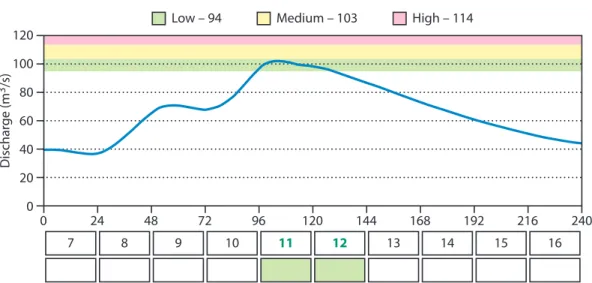
Is a forecast which first predicts 10 m3/s above a “medium” warning level (of let’s

10

say 100 m3/s ) and then 5 m3/s above inconsistent? How much does a probabilis-tic forecast have to change to be inconsistent?

2. Involve your end users in developing inconsistency forecast products

It is important that the way one decides to illustrate and demonstrate inconsis-tency is developed in a close relationship with the end user. Similar to a warning

15

system, these types of products cannot be designed at a scientist’s/forecaster’s desk alone.

3. Establish the magnitude of inconsistency and its dependency on catchment

loca-tion, hydrological and meteorological attributes.

Inconsistency will heavily depend on catchment properties such as catchment

20

response time. Flash flood forecasts on the medium range will be highly incon-sistent. In contrast forecasts which rely on a longer channel routing process with ample opportunity to be updated will exhibit less inconsistency (although perhaps at least in some dimensions, such as the size of the flood peak, its timing or the resulting spatial inundation pattern it may well be much more uncertain).

Inconsis-25

(13)

HESSD

8, 1225–1245, 2011

chain

Title Page

Tables Figures

◭ ◮

Back Close

Full Screen / Esc

Discussion

P

a

per

|

Dis

cussion

P

a

per

|

Discussion

P

a

per

|

Discussio

n

P

a

per

|

4. Make it a clear part of your decision making and communication framework

a. Establish the nature and magnitude of inconsistency with which you and your

end users are comfortablein issuing decisions/warnings.

b. Anticipate forecast inconsistency in your decision making (rather than just

reacting to it in a post event analysis setting). This means, if you expect high

5

inconsistency because of the season or domain in which you are working, make sure that you anticipate in your decision making and communication process that it could happen.

c. Clearly communicate in your warnings and decisions the level of

inconsis-tency at a level appropriate to the end user. As illustrated above,

communi-10

cation has to be targeted and not necessarily “numerical” (see also section on quantifying inconsistency). A good (but as yet unanswered) question is whether it would be better to be able to add this to the total uncertainty of your system in your communication process or whether it needs to be treated and communicated separately. This will be strongly end-user dependent. For

un-15

trained end-users all sources of uncertainty may best be folded into a single presentation, for trained end-users, which have to rely on additional decision making processes, the separation of uncertainty sources is vital.

d. If you have issued a warning and forecasts become inconsistent, do not

change your warning. Make clear what you expect the end-user to do.

Inves-20

tigate the source of the inconsistency.

e. If you have issued no warning and forecasts become inconsistent, do not

issue a warning. Make clear what you expect the end-user to do. Investigate

the source of the inconsistency. This may of course depend on the type of threshold: if there is a high threshold, then do nothing, but if you are issuing

25

(14)

HESSD

8, 1225–1245, 2011

chain

Title Page

Tables Figures

◭ ◮

Back Close

Full Screen / Esc

Discussion

P

a

per

|

Dis

cussion

P

a

per

|

Discussion

P

a

per

|

Discussio

n

P

a

per

|

f. Above all: Do not confuse end-users unless they are clearly involved in the process and understand what you are talking about (and you understand what they want from you!).

8 Conclusion

Flood forecasting based on numerical weather predictions remains a relatively new

5

field and using probabilistic forecasts is an even younger discipline and hence the guidelines above are only a very first step to initiate the discussion in this field. We ex-pect them to be evaluated and revised. We encourage all flood forecasters researching and practising in this area to routinely evaluate the inconsistency in their forecasts.

Is it a curse or blessing? We believe that it is a blessing in that it doesn’t lull us into

10

a false sense of “reliability” and it is better to know and actively approach all possible levels of uncertainty. However, aperfect systemwould have no issues with unreliability and it complicates our decision making and communication framework. If we could honestly choose, we would prefer not to have any inconsistency in our forecast rather than learning to live with it. In that sense it is a curse.

15

References

Bartholmes, J. C., Thielen, J., Ramos, M. H., and Gentilini, S.: The european flood alert system EFAS – Part 2: Statistical skill assessment of probabilistic and deterministic operational forecasts, Hydrol. Earth Syst. Sci., 13, 141–153, doi:10.5194/hess-13-141-2009, 2009. Beven, K. J.: A manifesto for the equifinality thesis, J. Hydrol., 320(1–2), 18–36, 2006.

20

Clements, M. P.: Evaluating the rationality of fixed-event forecasts, J. Forecast., 16, 225–239, 1997.

Clements, M. P. and Taylor, N.: Robustness of fixed-event forecast rationality, J. Forecast., 20(4), 285–295, 2001.

Cloke, H. L. and Pappenberger, F.: Ensemble flood forecasting: a review, J. Hydrol., 375(3–4),

25

(15)

HESSD

8, 1225–1245, 2011

chain

Title Page

Tables Figures

◭ ◮

Back Close

Full Screen / Esc

Discussion

P

a

per

|

Dis

cussion

P

a

per

|

Discussion

P

a

per

|

Discussio

n

P

a

per

|

Cloke, H. L., Thielen, J., Pappenberger, F., Nobert, S., Salamon, P., Buizza, R., B ´alint, G., Ed-lund, C., Koistinen, A., de Saint-Aubin, C., Viel, C., and Sprokkereef, E.: Progress in the im-plementation of hydrological ensemble prediction systems (HEPS) in Europe for operational flood forecasting, ECMWF Newsletter, 121, 20–24, www.ecmwf.int/publications/newsletters/ pdf/121.pdf, last access: 25 January 2011, 2009.

5

Dalcher, A., Kalnay, E., and Ho_ffman, R. N.: Medium range lagged average forecasts, Mon. Weather Rev., 116, 402–416, 1988.

Davies, A. and Demeritt, D.: Cost-benefit analysis and the politics of valuing the environment, Radical Statist., 73, 24–33, 2000.

Dedieu, F.: Alerts and catastrophes: the case of the 1999 storm in France, a treacherous risk,

10

Sociol. Trav., 52(1), 1–21, doi:10.1016/j.soctra.2010.06.001, 2010.

Demeritt, D., Cloke, H., Pappenberger, F., Thielen, J., Bartholmes, J., and Ramos, M.-H.: En-semble predictions and perceptions of risk, uncertainty, and error in flood forecasting, Envi-ron. Hazards, 7, 115–127, doi:10.1016/j.envhaz.2007.05.001, 2007.

Demeritt, D., Nobert, S., Cloke, H., and Pappenberger, F.: Challenges in communicating and

15

using ensembles in operational flood forecasting, Meteorol. Appl., 17, 209–222, 2010. Ehret, U.: Convergence index: a new performance measure for the jumpiness of operational

rainfall forecasts, in: 30th ICAM, Rastatt, May 2009, 152–153, 2009.

Faulkner, H., Parker, D., Green, C., and Beven, K.: Developing a translational discourse to communicate uncertainty in flood risk between science and the practitioner, Ambio, 36(7),

20

692–703, 2007.

Gupta, H., Sorooshian, S., Gao, X., Imam, B., Hsu, K.-L., Bastidas, L., Li, J., and Mahani, S.: The challenge of predicting flash floods from thunderstorm rainfall, Philos. T. Roy. Soc. A, 360, 1363–1371, 2002.

Hamill, T. M.: Evaluating forecasters’ rules of thumb: a study of D(Prog)/Dt, Weather Forecast.,

25

18, 933–937, 2003.

Hoffman, R. N. and Kalnay, E.: Lagged average forecasting, an alternative to monte-carlo forecasting, Tellus A, 35, 100–118, 1983.

Laio, F. and Tamea, S.: Verification tools for probabilistic forecasts of continuous hydrological variables, Hydrol. Earth Syst. Sci., 11, 1267–1277, doi:10.5194/hess-11-1267-2007, 2007.

30

(16)

HESSD

8, 1225–1245, 2011

chain

Title Page

Tables Figures

◭ ◮

Back Close

Full Screen / Esc

Discussion

P

a

per

|

Dis

cussion

P

a

per

|

Discussion

P

a

per

|

Discussio

n

P

a

per

|

Probability and Statistics, New Orleans, LA, Am. Meteorol. Soc., 9.4. available at http: //ams.confex.com/ams/pdfpapers/134204.pdf, last access: 25 January 2011, 2008.

MacKenzie, D.: Inventing Accuracy: an Historical Sociology of Nuclear Missile Guidance, MIT Press, Cambridge, MA, 1990.

Mills, T. C. and Pepper, G. T.: Assessing the forecasters: an analysis of the forecast records

5

of the treasury, the London Business School and the National Institute, Int. J. Forecast., 15, 247–257, 1999.

Murphey, A. H.: The value of climatological, categorical and probabilistic forecasting the cost-loss ratio situation, Mon. Weather Rev., 105, 803–816, 1977.

Nobert, S., Demeritt, D., Cloke, H. L.: Using ensemble predictions for operational flood

fore-10

casting: lessons from Sweden, J. Flood Risk Manage., 3(1), 7279, doi:10.1111/j.1753-318X.2009.01056.x, 2010

Nordhaus, W. D.: Forecast e_fficiency: concepts and applications, Rev. Econ. Stat., 69, 667– 674, 1987.

Palmer, T. N. and Tibaldi, S.: On the prediction of forecast skill, Mon. Weather Rev., 116, 2453–

15

2480, 1988.

Pappenberger, F., Bartholmes, J., Thielen, J., Cloke, H. L., Buizza, R., and de Roo, A.: New di-mensions in early flood warning across the globe using grand-ensemble weather predictions, Geophys. Res. Lett., 35, L10404, doi:10.1029/2008GL033837, 2008.

Pappenberger, F., Bogner, K., Wetterhall, F., He, Y, Cloke, H. L., and Thielen, J.: Forecast

con-20

vergence score: a forecasters approach to analysing hydro-meteorological forecast systems, Adv. Geosci., 9, 1-6, doi:10.5194/adgeo-9-1-2011, 2011.

Persson, A. and Grazzini, F.: User guide to ECMWF forecast products, available at http://www. ecmwf.int/products/forecasts/guide/index.html, last access: 25 January 2011, 2007.

Ramos, M. H., Mathevet, T., Thielen, J., and Pappenberger, F.: Communicating uncertainty

25

in hydro-meteorological forecasts: mission impossible?, Meteorol. Appl., 17(2), 223–235, 2010.

Richardson, D. S.: Skill and economic value of the ECMWF ensemble prediction system, Q. J. Roy. Meteor. Soc., 126, 649–668, 2000.

Roebber, P. J.: Variability in successive operational model forecasts of maritime cyclogenesis,

30

Weather Forecast., 5, 586–595, 1990.

(17)

HESSD

8, 1225–1245, 2011

chain

Title Page

Tables Figures

◭ ◮

Back Close

Full Screen / Esc

Discussion

P

a

per

|

Dis

cussion

P

a

per

|

Discussion

P

a

per

|

Discussio

n

P

a

per

|

Ruth, D. P., Glahn, B., Dagostaro, V., and Gilbert, K.: The performance of MOS in the digital age, Weather Forecast., 24(2), 504–519, 2009.

Shackley, S. and Wynne, B.: Integrating knowledges for climate change: pyramids, nets and uncertainties’, Global Environ. Change, 5, 113–126, 1995.

Slovic, P.: Perception of risk, Science, 236, 280–285, 1987.

5

Thielen, J., Bartholmes, J., Ramos, M.-H., and de Roo, A.: The European Flood Alert System – Part 1: Concept and development, Hydrol. Earth Syst. Sci., 13, 125–140, doi:10.5194/hess-13-125-2009, 2009a.

Thielen, J., Bogner, K., Pappenberger, F., Kalas, M., del Medico, M., and de Roo, A.: Monthly-, medium- and short range flood warning: testing the limits of predictability, Meteorol. Appl.,

10

16(1), 77–90, 2009b.

(18)

HESSD

8, 1225–1245, 2011

chain

Title Page

Tables Figures

◭ ◮

Back Close

Full Screen / Esc

Discussion

P

a

per

|

Dis

cussion

P

a

per

|

Discussion

P

a

per

|

Discussio

n

P

a

per

|

Table 1. Inconsistent threshold exceedance according to Fig. 1b. The rows indicate the date and time that the forecast was issued and the columns indicate the date for which the forecast was issued.

Forecast day 23 24 25 26 27 28 29 30

X

31 01 02 03 04

2010-03-22

2010-03-23

2010-03-24

2010-03-25

2010-03-26

2010-03-27

2010-03-28

2010-03-29

2010-03-30

(19)

HESSD

8, 1225–1245, 2011

chain

Title Page

Tables Figures

◭ ◮

Back Close

Full Screen / Esc

Discussion

P

a

per

|

Dis

cussion

P

a

per

|

Discussion

P

a

per

|

Discussio

n

P

a

per

|

Table 2. Number of ensemble members (out of 51) exceeding a high alert level. The rows indicate the date and time that the forecast was issued and the columns indicate the date for which the forecast was issued.

Forecast day 11 12 13 14 15 16 17 18 19 20

5 11 5 1 1

33 25 5 5 2

45 50

47 21 21 1 1 1

41 31 5 10 12

45 7 7 7

51 28 21 12

11 6

14

2

30

35

5 20 11 1

21 22 23

2010-10-11 00:00

2010-10-11 12:00

2010-10-12 00:00

2010-10-12 12:00

2010-10-13 00:00

2010-10-13 12:00

2010-10-14 00:00

(20)

HESSD

8, 1225–1245, 2011

chain

Title Page

Tables Figures

◭ ◮

Back Close

Full Screen / Esc

Discussion

P

a

per

|

Dis

cussion

P

a

per

|

Discussion

P

a

per

|

Discussio

n

P

a

per

|

Discharge [m

3S −1]

Discharge [m

3S −1]

Discharge [m

3S −1]

Discharge [m

3S −1]

03/25 03/26 03/27 03/28 03/29 03/30 03/31 04/01 04/02 04/03 04/04 20

40 60 80 100

Forecast issued on the 20020324

Time

03/25 03/26 03/27 03/28 03/29 03/30 03/31 04/01 04/02 04/03 04/04 20

40 60 80 100

Time

03/25 03/26 03/27 03/28 03/29 03/30 03/31 04/01 04/02 04/03 04/04 20

40 60 80 100

Time

03/25 03/26 03/27 03/28 03/29 03/30 03/31 04/01 04/02 04/03 04/04 20

40 60 80 100

Time

(i)

(ii)

(iii)

(iv)

(21)

HESSD

8, 1225–1245, 2011

chain

Title Page

Tables Figures

◭ ◮

Back Close

Full Screen / Esc

Discussion

P

a

per

|

Dis

cussion

P

a

per

|

Discussion

P

a

per

|

Discussio

n

P

a

per

|

120

0

7

24 48 72 96 120 144 168 192 216 240

8 9 10 11 12 13 14 15 16

100

80

60

Dischar

ge (m

3/s)

40

20

0

Low – 94 Medium – 103 High – 114