A panel data approach to economic forecasting: the bias-corrected average forecast

No _{642 ISSN 0104-8910}

A Panel Data Approach to Economic

Forecasting: The Bias–Corrected Average

Forecast

Os artigos publicados são de inteira responsabilidade de seus autores. As opiniões

neles emitidas não exprimem, necessariamente, o ponto de vista da Fundação

A Panel Data Approach to Economic

Forecasting: The Bias-Corrected Average

Forecast

João Victor Issler

Luiz Renato Lima

Graduate School of Economics – EPGE

Getulio Vargas Foundation

email: jissler@fgv.br and luizr@fgv.br

First Draft: December, 2006.

Abstract

In this paper, we propose a novel approach to econometric forecast-ing of stationary and ergodic time series within a panel-data frame-work. Our key element is to employ the bias-corrected average fore-cast. Using panel-data sequential asymptotics we show that it is po-tentially superior to other techniques in several contexts. In particular,

We are especially grateful to Ra¤aella Giacomini, Clive Granger, Marcelo Moreira, Zhijie Xiao, and Hal White, for their suggestions regarding the initial idea of the paper. We also bene…ted from comments given by Marcelo Fernandes, Marcelo Medeiros, and from the participants of the conference “Econometrics in Rio.” We thank Claudia Rodrigues for research assistance and gratefully acknowledge support given by CNPq-Brazil, CAPES, and Pronex. João Victor Issler thanks the hospitality of the Rady School of Management, and the Department of Economics of UCSD, where parts of this paper were written. The usual disclaimer applies.

it delivers a zero-limiting mean-squared error if the number of fore-casts and the number of post-sample time periods is su¢ciently large. We also develop a zero-mean test for the average bias. Monte-Carlo simulations are conducted to evaluate the performance of this new technique in …nite samples. An empirical exercise, based upon data from well known surveys is also presented. Overall, these results show promise for the bias-corrected average forecast.

Keywords: Panel-Data Econometrics, Pooling of Forecasts, Forecast Combination Puzzle, Common Features.

J.E.L. Codes:C14, C32, C33, C53, G11.

1

Introduction

Bates and Granger(1969) made the econometric profession aware of the bene-…ts of forecast combination when a limited number of forecasts is considered. The widespread use of di¤erent combination techniques has lead to an inter-esting puzzle from the econometrics point of view – the well known forecast combination puzzle: if we consider a …xed number of forecasts (N <1), combining them using equal weights (1=N) fare better than using “optimal weights” constructed to outperform any other forecast combination.

yet been given a full asymptotic treatment is that forecasting is frequently thought to be a time-series experiment, not a panel-data experiment. As far as we know, despite its obvious bene…ts, there has been no work where the pooling forecasts was considered in a panel-data context, with the number of forecasts (N) and time-series observations(T) diverging without bounds. In this paper, we propose a novel approach to econometric forecasting of stationary and ergodic series within a panel-data framework. First, we decompose individual forecasts into three components: the series being fore-cast, a time-invariant forecast bias, and a zero-mean forecast error. We show that the series being forecast is acommon feature of all individual forecasts; see Engle and Kozicki(1993). Second, when N; T _{! 1}, and we use stan-dard tools from panel-data asymptotic theory, we show that the pooling of forecasts delivers optimal limiting forecasts in the sense that they have a zero mean-squared error. The key element of this result is the use of the

bias-corrected average forecast – equal weights in combining forecasts cou-pled with a bias-correction term. The use of equal weights avoids estimating forecast weights, which contributes to reduce forecast variance, although po-tentially at the cost of an increase in bias. The use of a bias-correction term eliminates any possible detrimental e¤ect arising from equal weighting. One important element of our technique is to use the forecast combination puzzle to our advantage, but now in an asymptotic context.

The use of the bias-corrected average forecast is a parsimonious choice in forecasting that delivers optimal forecasts in a mean-squared error sense – zero limiting mean-squared error. The only parameter we need to estimate is the mean bias, which requires the use of the sequential asymptotic approach developed by Phillips and Moon (1999). Indeed, the only way we could increase parsimony in our framework is by doing without any bias correction. To test the usefulness of performing bias correction, we developed a zero-mean test for the average bias which draws upon the work of Conley (1999) on random …elds.

been panel-data research on forecasting focusing on pooling of information; see Stock and Watson (1999 and 2002a and b) and Forni et al. (2000, 2003). The former is related to forecast combination and operates a reduction on the space of forecasts. The latter operates a reduction on a set of highly correlated regressors. In principle, forecasting can bene…t from the use of both procedures. However, the payo¤ of pooling forecasts is greater than that of pooling information: while pooling information delivers optimal forecasts in the mean-squared error sense (Stock and Watson), it cannot drive the mean-squared forecast error to zero as the pooling of forecasts can.

One important element of our technique is the introduction of a bias-correction term. If a WLLN applies to a equal-weight forecast combination, we cannot guarantee a non-zero mean-squared error in forecasting, since the limit average bias of all forecasts may be non-zero. In this context, one inter-esting question that can be asked is the following: why are forecasts biased? From an economic standpoint, Laster, Bennett and Geoum (1999) show that professional forecasters behave strategically (i.e., they bias forecasts) if their payo¤s depend mostly on publicity from the forecasts than from forecast-accuracy itself. Since one way to generate publicity is to deviate from a consensus (average) forecast, rewarding publicity may induce bias. From an econometric point of view, Patton and Timmermann (2006) consider an addi-tional reason for the existence of bias in forecasts: what may look like forecast bias under a speci…c loss function may be just the consequence of the fore-caster using a di¤erent loss function in producing the forecast1_{. Hoogstrate,}

Palm and Pfann (2000) show that pooling cross-sectional slopes can help in forecasting. One of the potential reasons why this procedure works in practice is that only cross-sectional slopes are pooled, not individual e¤ects, showing that the latter may be working as a bias-correction device. A …nal reason for bias in forecasts is non-stationarity of the variable being forecast or of a subset of the conditioning variables. This is explored by Hendry and

1_{Also, Clements and Hendry’s (1999) work on intercept correction can be viewed as a}

Clements (2002) and Clements and Hendry (2006).

Given that important forecast studies are motivated by bias in forecast-ing, it seems desirable to build a forecasting device that incorporates bias correction. We view the introduction of the bias-corrected average forecast as one of the original contributions of this paper. The way we estimate the bias-correction term relies on the use of a forecast-speci…c component to cap-ture the bias in individual forecasts. Of course, this can only be fully studied asymptotically within a panel-data framework, which reinforces our initial choice of approach.

The ideas in this paper are related to research done in two di¤erent …elds. From econometrics, it is related to the common-features literature after En-gle and Kozicki (1993). Indeed, we attempt to bridge the gap between a large literature on common features applied to macroeconomics, e.g., Vahid and Engle (1993, 1997), Engle and Issler(1995), Issler and Vahid (2001, 2006) and Vahid and Issler (2002), and the econometrics literature on forecasting related to common factors, forecast combination, bias correction, and struc-tural breaks, perhaps best represented by the work of Bates and Granger (1969), Granger and Ramanathan(1984), Forni et al. (2000, 2003), Hendry and Clements (2002), Stock and Watson (2002a and b), Elliott and Tim-mermann (2003, 2004, 2005), and, more recently, by the excellent surveys of Clements and Hendry (2006), Stock and Watson (2006), and Timmer-mann (2006) – all contained in Elliott, Granger and TimmerTimmer-mann (2006). From …nance and econometrics, our approach is related to the work on fac-tor analysis when the number of assets is large, to recent work on panel-data asymptotics, and to panel-data methods focusing on …nancial applications, perhaps best exempli…ed by the work of Ross (1976), Chamberlain and Roth-schild (1983), Connor and Korajzcyk (1986, 1993), Phillips and Moon (1999), Bai and Ng (2002, 2004), Bai (2005), and Pesaran (2005), and Araujo, Issler and Fernandes (2006).

the Appendix. Section 3 presents the results of a Monte-Carlo experiment. Section 4 presents an empirical analysis using the methods proposed here, confronting the performance of the bias-corrected average forecast with that of other types of forecast combination. Section 5 concludes.

2

Econometric Setup

Suppose that we are interested in forecasting a weakly stationary and ergodic univariate process _fYtg using a large number of forecasts that will be

com-bined to yield an optimal forecast in the mean-squared error (MSE) sense. These forecasts could be the result of using several econometric models that need to be estimated prior to forecasting, or the result of using no formal econometric model at all, e.g., just the result of an opinion poll on the vari-able in question using a large number of individual responses.

We consider 3 consecutive distinct time periods, where time is indexed by t = 1;2; : : : ; T1: : : ; T2: : : ; T. The period from t = 1;2; : : : ; T1 is labeled

the “estimation sample,” where models are usually …tted to forecast Yt, if

that is the case. The period from t = T1 + 1; : : : ; T2 is labeled the

post-model-estimation or “training sample”, where realizations of Yt are usually

confronted with forecasts produced in the estimation sample, if that is the case. The …nal period is t = T2 + 1; : : : ; T, where genuine out-of-sample

forecasting is entertained, bene…ting from the results obtained during the training sample. In what follows, we let T2 be O(T). In order to guarantee

that the number of observations in the training sample will go to in…nity at rate T, we let T1 be O(1). Hence, asymptotic results will not hold for the

estimation sample.

Regardless of whether forecasts are the result of a poll or of the estimation of econometric models, we label forecasts ofYt, computed using conditioning

sets laggedh periods, byfh

i;t,i= 1;2; : : : ; N. Therefore,fi;th areh-step-ahead

forecasts and N is either the number of models estimated to forecast Yt or

In what follows we will let N go to in…nity, which raises the question of whether this is plausible in our context. On the one hand, if forecasts are the result of estimating econometric models, they will di¤er across i if they are either based upon di¤erent conditioning sets or upon di¤erent functional forms of the conditioning set (or both). Since there is an in…nite number of functional forms that could be entertained for forecasting, this gives an in…nite number of possible forecasts. On the other hand, if forecasts are the result of a survey, although the number of responses is bounded from above, for all practical purposes, if a large enough number of responses is obtained, then the behavior of forecast combinations will be very close to the limiting behavior when N _{! 1}.

We will focus on the following decomposition ofYt:

Yt=fi;th Ki "i;t; i= 1;2; : : : ; N; t > T1; (1)

whereKi is a time-invariant forecast bias of modelior of respondenti. This

makes the error term "i;t a zero-mean process, although it will be serially

correlated in general. Because fh

i;t is anh-step-ahead forecast, Ki and"i;t are

respectively the h-step-ahead forecast bias and the forecast error associated with either model i or respondent i. Here, to simplify notation, we do not use an h superscript on Ki and "i;t, although they clearly depend on h.

At this point, it is desirable to discuss the nature of the term Ki. In

particular, it is important to explain why we need to model it, which is related to the question of why we cannot focus solely on unbiased forecasts, for which Ki = 0. At …rst sight, (1) looks like an identity, but it is not,

since we may also have a time-varying bias term. Therefore, the role of Ki

in (1) is to capture the long-run e¤ect in the time dimension of model-bias misspeci…cation (econometric models ofYt) or the long-run e¤ect in the time

dimension of the bias of respondenti. When considering econometric models, it is natural to assume that we do not know the data-generating process ofYt.

Therefore, all models that we might consider are inherently misspeci…ed. In this case, Ki captures the long-run e¤ect, in the time dimension, of

some of the surveyors may gain something by having a biased forecast. An interesting example in …nance is that of a bank selling an investment fund. In this case, the bank’s forecast of the fund return may be upward-biased simply because it may use this forecast as a marketing strategy to attract new clients; see Laster, Bennett and Geoum (1999). Patton and Timmermann (2006) consider an additional reason for the existence of Ki – the fact that

there is uncertainty about the type of loss function used by forecasters in forming a speci…c forecast. There, forecasts that are unbiased under the loss function used by the forecaster may look biased under a di¤erent loss function.

Next, we have an assumption on howKi relates to "i;t.

Assumption 1: We assume thatE("i;tjKi) = 0, for all t and thatKi is an

identically distributed random variable in the cross-sectional dimen-sion, but not necessarily independent2_{, i.e.,}

Ki id(B; 2k); (2)

where B and 2

k are respectively the mean and variance of Ki. It is

important to distinguish betweenKi and its realizationki. In the

time-series dimension,ki has no variation, therefore, it is a …xed parameter.

The error term "i;t is assumed to be weakly stationary and ergodic,

re-‡ecting the fact that, if forecasts are such that "i;t is not weakly

station-ary and ergodic, then these forecasts could be simply discarded3_{. Because}

forecasts are computed h-steps ahead, forecast errors are serially correlated in general even if they are unbiased. Forecast errors are also likely to be

2_{The assumption of dependence is consistent with the idea that forecasters learn from}

one another by meeting, discussing, debating, and reading each other’s analyses. Through their ongoing interactions, forecasters maintain a current, collective understanding of where the economy is most likely heading and its upside and downside risks.

3_{It is beyond the scope of this paper to discuss forecast combination for non-stationary}

processes. Also, note that althoughYtand"i;t are ergodic for the mean,fi;th is non ergodic

cross-sectionally correlated, since the information set used by di¤erent mod-els tends to overlap and poll responses tend to be similar for respondents with similar characteristics. In order to limit the degree of time-series and cross-sectional dependence of the errors, we assume the following:

Assumption 2: Let"_t= ("_1;t; "_2;t; ::: "_N;t)0 be an N 1vector stacking the

errors associated with all possible forecasts. Then, the vector process

f"_tg is assumed to be covariance-stationary and ergodic for the …rst

and second moments, uniformly onN. Further, de…ning as i;t ="i;t Et 1("i;t), the innovation of "i;t, whereEt 1( )denotes the conditional

expectation operator, we assume that

lim

N!1

1

N2

N X

i=1

N X

j=1

E i;t j;t = 0: (3)

Assumption 2 controls the degree of time-series and cross-sectional de-pendence in the data. It does not rule out errors displaying conditional heteroskedasticity, since the latter can coexist with the assumption of weak stationarity; see Engle (1982). A similar assumption is made in Araujo, Issler and Fernandes (2006) to control the time-series and the cross-sectional de-cay within the framework of factor models applied to …nance. Following the forecasting literature with large N and T, e.g., Stock and Watson (2002b), and the …nancial econometric literature, e.g., Chamberlain and Rothschild (1983), the condition lim

N!1

1

N2

PN i=1

PN

j=1 E i;t j;t = 0simply controls the

degree of cross-sectional dependence present in forecast errors. It is noted by Bai (2005, p. 6), that Chamberlain and Rothschild’s cross-sectional error decay requires:

lim

N!1

1

N N X

i=1

N X

j=1

E i;t j;t <1: (4)

2 has a less restrictive condition than those commonly employed for factor models. It guarantees convergence in probability of cross-sectional means, which is why we use it here.

We start the discussion on forecast combination by solving (1) forfh i;t:

fh

i;t =Yt+Ki+"i;t; i= 1;2; : : : ; N; t > T1: (5)

Equation (5) shows that we can decompose all forecasts into a common com-ponent Yt, and two idiosyncratic components Ki and "i;t. The series being

forecast (Yt) is a common feature, in the sense of Engle and Kozicki(1993),

of all forecasts. For any two series, a common feature exists if it is present in both of them and can be removed by linear combination. Here, subtracting any two forecasts eliminates Yt. Araujo, Issler and Fernandes (2006) exploit

this property to develop an estimator for the stochastic discount factor within a panel-data context. Here, we also exploit this property of Ytin devising an

optimal predictor for its realizations. We now state our …rst result.

Proposition 1 If Assumptions 1 and 2 hold, then, the bias-corrected average

forecast obeys plim

N!1

1

N N X

i=1

fh i;t

1

N N X

i=1

ki !

=yt and

lim

N!1MSE

1

N N X

i=1

fh i;t N1

N X

i=1

ki !

= 0, t > T1, where MSE( ) denotes the

mean-squared error in forecasting Yt, yt denotes period-t realization of Yt,

and ki denotes the realization of Ki.

Proof. See Appendix.

bias-corrected equal weights (1=N) will both have a zero MSE. However, in practice, one cannot resort to “optimal population weights,” but rather has to estimate “optimal weights” from the data. Since the estimation period is …xed, t= 1;2; : : : ; T1 (although the training period is not), the performance

of “optimal estimated weights” will not be as good as that of “optimal popu-lation weights,” which explains the poor performance of “optimal estimated weights” compared with bias-corrected equal weights. From that perspective, there is no “forecast-combination puzzle.”

Understanding the puzzle required using a weak law-of-large-numbers in a panel-data context. We see this as a major advantage of our approach vis-à-vis the commonly employed time-series approach with …xedN. Only in a panel-data framework can we formally state a weak law-of-large-numbers for forecast combinations and take full advantage of asymptotic results in both

N and T. The lack of a broad of use of panel-data analysis in forecasting so far has limited our understanding of important phenomena in this literature. Of course, the lead of Stock and Watson(1999 and 2002a and b) and Forni et al. (2000, 2003) towards panel data has shed light on several important results on pooling information. We hope that our work will do the same as far as the pooling of forecasts is concerned.

One important feature of _N1

N X

i=1

fh i;t N1

N X

i=1

ki is that it is unfeasible, since

we do not observe the ki’s. Therefore, below we propose replacing ki by a

consistent estimator. The underlying idea behind the consistent estimator of

ki is that in the training sample one observes the realizations of Ytand of the

double-index process fh

i;t,i= 1:::N, and T1 < t < T2. Hence, one can form a

panel of forecasts:

fh

i;t yt =ki+"i;t; i= 1;2; : : : ; N; T1 < t < T2; (6)

where i indexes forecasts, t indexes time, and it becomes obvious that ki

represents the …xed e¤ect on this panel. It is natural to exploit this property of ki in constructing a consistent estimator. This is exactly the approach

It does not depend on any distributional assumption on Ki id(B; 2k)

and it does not depend on any knowledge of the models used to compute the forecasts fh

i;t. This feature of our approach widens its application to

situations where the “underlying models are not known, as in a survey of forecasts” – Kang (1986); see also our empirical-application section.

Due to the nature of our problem – large number of forecasts – and the nature of ki in (6) – time-invariant bias term – we need to consider large N, large T asymptotic theory to devise a consistent estimator for ki. Panels

with such a character are di¤erent from largeN, smallT panels. In order to allow the two indices N and T to pass to in…nity jointly, we could consider a monotonic increasing function of the type T =T(N), known as diagonal-asymptotic method; see Quah (1994) and Levin and Lin (1993). One draw-back of this approach is that the limit theory that is obtained depends on the speci…c relationship considered inT =T(N). A joint-limit theory allows both indices (N and T) to pass to in…nity simultaneously without imposing any speci…c functional-form restriction. Despite that, it is substantially more di¢cult to derive and will usually apply only under stronger conditions, such as the existence of higher moments.

Searching for a method that allows robust asymptotic results without imposing too many restrictions (on functional relations and the existence of higher moments), we consider the sequential asymptotic approach developed by Phillips and Moon (1999). There, one …rst …xes N and then allows T

to pass to in…nity using an intermediate limit. Phillips and Moon write sequential limits of this type as (T; N _{! 1})seq.

In order to clarify the idea behind sequential asymptotics, consider the following double-indexed process:

XN;T =

1

kN N P i=1

Zi;T;

and denote by Zi the limit of Zi;T as T ! 1. Phillips and Moon derive

intermediate limit XN = _k1 N

N P i=1

Zi is found. Then, by lettingN ! 1and by

applying an appropriate limit theory to the standardized sumXN = _k1_N n P i=1

Zi,

the …nal sequential limit is obtained. When kN =N, this results in a

law-of-large numbers being applied. WhenkN =

p

N, this results in a central-limit theorem being applied.

In general, Phillips and Moon argue that a joint limit (N andT go to in…n-ity simultaneously) is a more robust result than a sequential limit. However, these two could be equivalent. Following the intuition behind the conver-gence of a double-indexed real-number sequence, they show that if …rst-stage convergence in the sequential limit holds uniformly on the other index, then the sequential limit is equivalent to a joint limit, e.g., if XN;T converges to XN uniformly in N, as T ! 1, then sequential limit of XN;T is the same

as the joint limit of XN;T. Sequential panel-data asymptotics were applied

in Phillips et al. (2001) and in Lima and Xiao (2007), among others. By using the sequential-limit approach, we can now state the second result of this paper.

Proposition 2 If Assumptions 1 and 2 hold, the feasible bias-corrected

av-erage forecast obeys plim (T;N!1_)seq

1 N N X i=1 fh i;t N1

N X i=1 b ki !

=yt and

lim

(T;N!1_)seqMSE

1 N N X i=1 fh i;t N1

N X i=1 b ki !

= 0, t > T1, where bki = _T1 PT_t=1fi;th

1

T PT

t=1yt is a consistent estimator of ki, as T ! 1.

Proof. See Appendix.

In what follows we make explicit the role ofBb, the consistent estimator of B proposed in the proof of Proposition 2..

Proposition 3 If Assumptions 1 and 2 hold, then, plim (T;N!1_)seq

b

B B = 0.

The results above provide important tools for largeN; T forecasting. To get optimal forecasts, in the MSE sense, one has to combine all forecasts using simple averaging, appropriately centering it by using a bias-correction term. It is important to stress that, even thoughN _{! 1}, the number of estimated parameters is kept at unity: Bb. This is a very attractive feature compared to models that combine forecasts estimating optimal weights. There the number of estimated parameters increases at the same rate asN, a clear disadvantage from the point of view of obtaining a small forecast variance.

The feasible bias-corrected average forecast can be made an even more parsimonious estimator ofytwhen there is no need to estimateB. Of course,

this raises the issue of whether B = 0, in which case the optimal forecast

becomes _N1

N X

i=1

fh

i;t – the simple forecast combination originally proposed by

Bates and Granger (1969). We next propose the following test statistic for

H0 :B = 0.

Proposition 4 Under the null hypothesis H0 :B = 0, the test statistic:

b

t= _pBb

b

V

d

! (T;N!1)seq N

(0;1);

where Vb is a consistent estimator of the asymptotic variance ofB = 1

N N X

i=1

ki.

Proof. See Appendix.

3

Monte-Carlo Study

We considered the following data-generating process (DGP):

Yt = Xt+ t

where _fXtg is an ARF IM A(1; d;0) process, in which (1 L)dXt = t,

(1 L) _t = t, and t iid N(0;1). We also assumed that t iid N(0;1) and _t and t are mutually independent. The data were generated

by using functions of the ARFIMA package (Doornik and Ooms, 2001) for Ox programming language. In particular, we set = 0:8, = 5 andd= 0:1,

0:4,0:49.

According to Beran (1998), one of the typical features of the above DGP (a stationary long-memory process) is that it generates local trends and cy-cles, but these are potentially spurious and disappear after some time. There-fore, for short sample sizes, we expect that this property will lead to poor forecasts since the estimated models will only capture the spurious local trend or cycle, which does not represent the true dynamics of Yt. For this

reason, we paid special attention to models that are estimated with a small sample. In this experiment, we considered the estimation sample to be as small asT1 = 30;60;120, which are sample sizes commonly found in applied

macroeconometrics.

As for the training sample,T2 T1, this experiment included T2 T1 =

30;60. Recall that T2 = O(T) and, therefore we need to increase T to

accommodate larger training samples. In this experiment, we set the number of out-of-sample observations as (T T2) = 10. Hence, when T1 = 30 and

T2 T1 = 30;the total sample sizeT will be equal to 70. If T1 = 30, but the

training samples goes up to 60, then T must be equal to 100, etc. We …tted the following auto-regressive distributed-lag models forYt,

Yt = c0 +

J P j=1

jYt j+ I P i=0 i

Xt i+ t (7)

f or J = 1;2; :::;6,

I = 1;2; :::;5:

explained below, in addition to the simple average forecast (equal weights

1=N without any bias correction):

1. We estimated each model using observations up to periodT1, which is

our estimation sample. The estimated models are next used to make one-step-ahead forecasts (h= 1) in the training sample, fromT1+ 1to

T2. These forecasts are then used to estimate the model bias and the

average bias. Without updating the estimation sample, each model is used to forecast observations from T2 + 1 to T. Finally, the

bias-corrected average forecasts is computed.

2. The same procedure as in 1 above is implemented without any bias correction: this is the simple average forecast combination.

3. After estimating all models in (7) using the estimation sample, the training sample is used to estimate the weights according to the follow-ing OLS regression:

ys =!0+ 30

P i=1

!itfi;s1 +"s, s=T1+ 1; :::T2, (8)

where f1

i;s is the one-step ahead forecast made by the i-th model for the s

-th observation in -the training sample. The estimated weights are used to compute the weighted-average forecast from T2 + 1 toT.

We then compute the MSE of the simple average forecast, the bias-corrected average forecast, and the weighted-average forecast for the peri-ods T2+ 1; :::; T. All the forecasts are one-step-ahead static forecasts, i.e.,

forecasts for t+ 1 used observed data forYt.

bias-corrected average forecast). The second is that of the weighted-average forecast (the MSE of the weighted-average forecast divided by that of the bias-corrected average forecast).

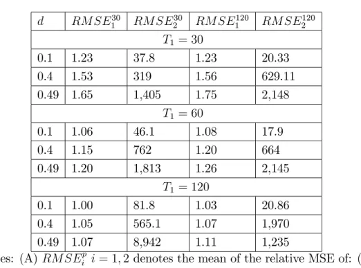
We report the mean of each distribution in Table 1. The notationRM SE_ip i = 1;2 denotes the mean of the relative MSE of the average forecast

(RM SE₁p) and weighted-average forecast (RM SE₂p). The superscript p in-dicates the number of observations in the training sample.

The results in Table 1 show that, for estimation sample as small as

T1 = 30, the bias-corrected average forecast outperforms the simple

aver-age forecast. In particular, such advantaver-age increases as the presence of long memory is stronger, that is, as the fractional-integration parameter d in-creases. Indeed, for d = 0:1, RM SE30

1 = 1:23, whereas RM SE130 = 1:65

when d = 0:49.4 _{The forecast can be improved if more observations are}

used in the training sample. For example, when 120 observations are used to compute the average bias, we obtain RM SE120

1 = 1:75for d= 0:49.

The good performance of the bias-corrected average forecast results from the fact that stationary long-memory processes generate local trends and cycles that disappear only after a long time. For short-estimation samples, the econometric models (7) will all include irrelevant regressors, which may lead to non-trivial forecast biases, the smaller the estimation sample. Of course, as the estimation sample increases, the coe¢cients of these irrelevant regressors will be approximately zero and we should expect the gains of bias correction to decrease. Our Monte-Carlo experiment shows that the method proposed in this paper can improve forecast accuracy by estimating and re-moving this short-sample forecast bias. As the estimation sample increases, say, to T1 = 120, the local trends and cycles become less important and

therefore the misspeci…cation problem diminishes.5 _{As a result, the}

econo-4_{Recall that a long-memory process is stationary as long as0< d <0:5.}

5_{As motivated by Hendry and Clements (2002), model bias can be corrected by}

metric models will give rise to small bias and, consequently, bias-correction will not be as important as in the case of a small estimation sample.

A striking result presented in Table 1 is the e¤ect of long memory on the performance of the weighted-average forecast. Such forecast method has the worst performance among the three methods considered. Its performance deteriorates signi…cantly when the fractional-integration parameter increases. This result suggests that local trends and cycles generated by a stationary long-memory process (along with a small estimation sample) strongly bias the estimation of the “optimal” weights used to compute the weighted-average forecast. In this way, the well-known forecast-combination puzzle may simply be a re‡ection of the potential misspeci…cation of econometric models used in forecasting.

4

Empirical Application

Professional forecasts guide market participants and inform them about fu-ture economic conditions. However, many analysts argue that forecasters might strategically bias forecasts as long as they receive economic incen-tives to do so. The importance of microeconomic incenincen-tives for forecasters and analysts is stressed by a number of empirical studies, such as Ehrbeck and Waldmann (1996), Graham (1999), Hong et al. (2000), Lamont (2002), Welch (2000), and Zitzewitz (2001).

In this section, we present an application of the method proposed here for the case of forecast surveys, focusing on two di¤erent surveys. Our re-sults show that bias correction can indeed help forecasting. We also test the hypothesis that professional forecasters behave strategically in a statistical sense, perhaps because they earn more from forecast publicity than from fore-cast accuracy. When this is accounted for, the bias-corrected average forefore-cast introduced in this paper outperforms simple forecast averages (consensus). It is important to stress that, although our techniques were conceived for a large

of our method even in a smallN; T environment. Also, the forecasting gains from bias correction, whenever the average forecast is biased, are non-trivial.

4.1

Philadelphia Fed’s Survey of Professional

Forecast-ers

In our …rst empirical application, we consider a panel data of individual re-sponses from the Philadelphia Fed’s Survey of Professional Forecasters avail-able at quarterly frequency. The forecasters in this Survey come largely from the business world and Wall Street. One important feature of this Survey is anonymity of the institution supplying a given forecast. This is designed to encourage forecasters to provide their best forecast without fearing the consequences of making mistakes.

For a long time it has been common knowledge that the average forecast usually performs better than alternative forecast combinations when survey data is used. In fact, Kang (1986) concludes that “A simple average should be used when underlying models are not known, as in a survey of forecasts...” In this section we show how a macroeconomist using survey data can use the bias-corrected average forecast to improve upon the consensus (average) forecast.

In order to construct our panel of forecasts, we have to consider the fact that many forecasters report missing values for di¤erent reasons, which is a problem in trying to obtain a long-balanced panel of forecasts. To that end, we included forecasters who reported nine consecutive one-step-ahead forecasts from 2002:4 to 2004:4. Hence, our time dimension is T = 9. To compute the average bias, we compared one-step-ahead forecasts with real-izations of the forecasting variables from 2002:4 through 2003:4, comprising5

observations. Therefore, we were left with observations from 2004:1 through 2004:4 for out-of-sample forecast evaluation (4observations).

rate, both seasonally adjusted. For CPI in‡ation we observed a maximum of N = 19 forecasters, whereas for the unemployment rate, we observed a maximum of N = 22 forecasters.

Table 2 exhibits the estimate of the sample average bias for CPI in‡ation and the Unemployment Rate. We also test whether the average bias is zero (p-values in parenthesis). Our estimates reveal a negative average bias for the annualized in‡ation rate and a positive bias for the unemployment rate. Both are statistically signi…cant at the 10% level, but only the unemployment average bias is signi…cant at the 5% level. This result suggests that we could use these average-bias estimates to improve forecasting, although we should expect a larger improvement in the case of unemployment. Indeed, the simple average forecast is 9% worse than the feasible bias-corrected average forecast for CPI in‡ation and 56% worse for the Unemployment Rate.

4.2

The Central Bank of Brazil’s “Focus Forecast

Sur-vey”

The “Focus Forecast Survey,” organized by the Central Bank of Brazil, is a unique panel database of forecasts. It collects forecast information on al-most 120 institutions, including commercial banks, asset managers and non-…nancial institutions, which are followed throughout time. Forecasts have been collected since 1998, which potentially can serve to approximate a large

N; T environment. Besides that, it also has the following desirable features: the anonymity of forecasters is preserved, although the names of the top-…ve forecasters for a given economic variable is released by the Central Bank of Brazil; forecasts are collected at di¤erent frequencies (monthly, semi-annual, annual), as well as at di¤erent forecast horizons (e.g., short-run forecasts are obtained forhfrom 1 to 12 months); there is a large array of macroeconomic time series included in the survey.

Consumer Price Index (CPI), computed by FIBGE. In order to obtain the largest possible balanced panel (N T), we usedN = 18 and a time-series sample period covering the period 2002:11 through 2006:3 (T = 41). Of course, in the case of a survey panel, there is no estimation sample. We chose the …rst 23 time observations to compute Bb – the average bias – leaving 18

time-series observations for out-of-sample forecast evaluation. The forecast horizon chosen was h = 6, this being an important horizon to determine future monetary policy within the Brazilian In‡ation-Targeting program.

The results of our empirical exercise are presented in Tables 3 and 4. They show that the average bias is positive for the 6-month horizon – about

0:075– and signi…cant at the10%level, with a p-value of0:09. Out-of-sample forecast comparisons between the simple average and the bias-corrected av-erage forecast show that the former has an MSE11% bigger than that of the latter.

5

Conclusions and Extensions

In this paper, we propose a novel approach to econometric forecasting of sta-tionary and ergodic series within a panel-data framework, where the number of forecasts and the number of time periods increase without bounds. The advantages of our approach are many. First, only in an asymptotic panel-data context we can fully understand why the pooling of forecasts works in practice. Second, we can also propose improvements on simple forecast-combination schemes – such as the simple forecast forecast-combination. Here, we propose the bias-corrected average forecast. Third, our techniques are ap-plicable in two important contexts: when forecasts are a result of model es-timation, and when they are the result of opinion polls. Fourth, the method proposed here is non-parameteric: it requires no distributional assumption whatsoever on the variables involved, and also no knowledge of the models used in forecasting.

components: the series being forecast, a time-invariant forecast bias, and a zero-mean forecast error. The series being forecast is viewed as a common featureof all individual forecasts. Standard tools from panel-data asymptotic theory are then used to devise an optimal forecasting combination that has a zero limiting mean-squared forecast error. This optimal forecast combina-tion uses equal weights and a bias-correccombina-tion term. The use of equal weights avoids estimating forecast weights, which contributes to reduce forecast vari-ance, although potentially at the cost of an increase in bias. The use of a bias-correction term eliminates any possible detrimental e¤ect arising from equal weighting. We label this optimal forecast as thebias-corrected average forecast.

In theory – largeN andT – the use of a bias-corrected average forecast is potentially superior to the use of any single forecast and is equal or superior to any other combining technique. Moreover, in practice – small N and/or

T – an important element of the use of the bias-corrected average forecast is that the forecast combination puzzle works to our advantage, now augmented with a bias-correction term. Hence, there will be situations in which we can improve upon the simple average forecast by using a bias-correction, and others which we cannot. Our framework o¤ers a statistical test for excluding the bias-correction term.

For reasons of space, we refrain from fully discussing here natural ex-tensions of our proposed method. A partial account of those includes the following:

1. In the panel of forecasts:

fi;th yt =ki+"i;t; i= 1;2; : : : ; N; T1 < t < T2; (9)

we imposed a unity coe¢cient foryt, but we could have had an

encom-passing panel-regression system:

fh

i;t = iyt+ki+"i;t; i= 1;2; : : : ; N; T1 < t < T2; (10)

where _i can be interpreted as the beta of forecast-model i vis-à-vis

yt. A natural hypothesis to test is H0 : i = 1, for all i, which can be

implemented using standard panel techniques.

2. There may be instances where forecast models produce forecasts that are too highly correlated. In theory, this may prevent a weak law-of-large-numbers from holding for the error terms. In this case we can combine pooling of information and pooling of forecasts:

fi;th yt =ki+ K X

k=1

i;kfk;t+ i;t; i= 1;2; : : : ; N; T1 < t < T2;

(11) where fk;t are zero-mean pervasive factors and, as is usual in factor

analysis, plim

N!1

1

N PN

i=1 i;t = 0. In this context, we implemented the following

decomposition:

"i;t = K X

k=1

i;kfk;t+ i;t; i= 1;2; : : : ; N; T1 < t < T2:

3. The …nal extension considered here is to allow for a time-varying bias term _t. In this case,

fh

i;t yt =ki+ t+"i;t; i= 1;2; : : : ; N; T1 < t < T2: (12)

The techniques of Fuller and Battese (1974) can be a starting point to generate consistent estimates of ki and t in a context where N and T

are large.

References

[1] Araujo, F., Issler, J.V. and Fernandes, M.(2006), “A Stochas-tic Discount Factor Approach to Asset Pricing Using Panel Data,” Working Paper: EPGE-FGV # 628, downloadable from http://epge.fgv.br/portal/arquivo/2155.pdf

[2] Bai, J., (2005), “Panel Data Models with Interactive Fixed E¤ects,” Working Paper: New York University.

[3] Bai, J., and S. Ng, (2002), “Determining the Number of Factors in Approximate Factor Models,” Econometrica, 70, 191-221.

[4] Bai, J. and S. Ng, (2004), “Evaluating Latent and Observed Factors in Macroeconomics and Finance,” Working Paper: University of Michigan.

[5] Beran, Jan, (1998), “Statistics for Long-Memory Processes.” Chapman and Hall – CRC.

[6] Chamberlain, Gary, and Rothschild, Michael, (1983). “Arbitrage, Fac-tor Structure, and Mean-Variance Analysis on Large Asset Markets,”

Econometrica, vol. 51(5), pp. 1281-1304.

[8] Clements, M.P. and D.F. Hendry, 2006, Forecasting with Breaks in Data Processes, in C.W.J. Granger, G. Elliott and A. Timmermann (eds.)

Handbook of Economic Forecasting, pp. 605-657, Amsterdam, North-Holland.

[9] Conley, T.G., 1999, “GMM Estimation with Cross Sectional Depen-dence,” Journal of Econometrics, Vol. 92 Issue 1, pp. 1-45.

[10] Connor, G., and R. Korajzcyk (1986), “Performance Measurement with the Arbitrage Pricing Theory: A New Framework for Analysis,”Journal of Financial Economics, 15, 373-394.

[11] Connor, G. and Korajczyk, R. (1993), “A test for the number of factors in am approximate factor structure,”Journal of Finance 48, 1263 - 1291.

[12] Doornik, J. and M. Ooms (2001), “A package for estimating, forecasting and simulating ar…ma models: Ar…ma package 1.01 for ox.” OX open source software..

[13] Ehrbeck, T., Waldman, R., 1996. Why are professional forecasters bi-ased? Agency versus behavioral explanations.Quarterly Journal of Eco-nomics 111, 21-40.

[14] Elliott, G., C.W.J. Granger, and A. Timmermann, 2006, Editors, Hand-book of Economic Forecasting, Amsterdam: North-Holland.

[15] Elliott, G. and A. Timmermann (2005), “Optimal forecast combination weights under regime switching”,International Economic Review, 46(4), 1081-1102.

[17] Engle, R.F. (1982), “Autoregressive Conditional Heteroskedasticity with Estimates of the Variance of United Kingdom In‡ation,”Econometrica, 50, pp. 987-1006.

[18] Engle, R. F., Issler, J. V., 1995, “Estimating common sectoral cycles,”

Journal of Monetary Economics, vol. 35, 83–113.

[19] Engle, R.F. and Kozicki, S. (1993). “Testing for Common Features”,

Journal of Business and Economic Statistics, 11(4): 369-80.

[20] Forni, M., Hallim, M., Lippi, M. and Reichlin, L. (2000), “The General-ized Dynamic Factor Model: Identi…cation and Estimation”, Review of Economics and Statistics, 2000, vol. 82, issue 4, pp. 540-554.

[21] Forni M., Hallim M., Lippi M. and Reichlin L., 2003 “The Generalized Dynamic Factor Model one-sided estimation and forecasting,” Journal of the American Statistical Association, forthcoming.

[22] Forni, M., M. Hallim, M. Lippi and L. Reichlin (2004), “The generalized factor model: consistency and rates”, Journal of Econometrics 119:231-255.

[23] Fuller, Wayne A. and George E. Battese, 1974, “Estimation of lin-ear models with crossed-error structure,” Journal of Econometrics, Vol. 2(1), pp. 67-78.

[24] Giacomini, Ra¤aella and Halbert White, 2006, “Tests of Conditional Predictive Ability,” Econometrica, vol. 74(6), pp. 1545-1578.

[25] Graham, J., 1999. Herding among investment newsletters: theory and evidence. Journal of Finance 54, 231-268.

[27] Hendry, D.F. and M.P. Clements (2002), “Pooling of forecasts”, Econo-metrics Journal, 5:1-26.

[28] Hong, H., Kubik, J.D., Solomon, A., 2000. Security analysts ´career concerns and herding of earning forecasts. RAND Journal of Economics

31, 121-144.

[29] Hoogstrate, Andre J., Franz C. Palm, Gerard A. Pfann, 2000, “Pooling in Dynamic Panel-Data Models: An Application to Forecasting GDP Growth Rates,” Journal of Business and Economic Statistics, Vol. 18, No. 3, pp. 274-283.

[30] Issler, J. V., Vahid, F., 2001, “Common cycles and the importance of transitory shocks to macroeconomic aggregates,” Journal of Monetary Economics, vol. 47, 449–475.

[31] Issler, J. V., Vahid, F., 2006, “The missing link: Using the NBER reces-sion indicator to construct coincident and leading indices of economic activity,”Annals Issue of the Journal of Econometrics onCommon Fea-tures, vol. 132(1), pp. 281-303.

[32] Kang, H. (1986), "Unstable Weights in the Combination of Forecasts,"

Management Science 32, 683-95.

[33] Lamont, O., 2002. Macroeconomic forecasts and microeconomic fore-casters. Quarterly Journal of Economics 114, 293-318.

[34] Levin, A., Lin, C.-F., 1993, “Unit root tests in panel data:asymptotic and …nite-sample properties,” UC San Diego: Unpublished Working Pa-per.

[36] Pesaran, M.H., (2005), “Estimation and Inference in Large Heteroge-neous Panels with a Multifactor Error Structure.” Working Paper: Cam-bridge University, forthcoming in Econometrica.

[37] Phillips, P.C.B., 1995, “Lecture Notes,” downloadable from the author’s webpage: Yale University.

[38] Phillips, P.C.B. and H.R. Moon, 1999, “Linear Regression Limit Theory for Nonstationary Panel Data,” Econometrica, vol. 67 (5), pp. 1057– 1111.

[39] Phillips, P.C.B., H.R. Moon and Z. Xiao, 2001, “How to estimate au-toregressive roots near unity,” Econometric Theory 17, 29-69.

[40] Quah, D., 1994, “Exploiting cross section variation for unit root infer-ence in dynamic data,” Economic Letters 44, 9–19.

[41] Ross, S.A. (1976), “The arbitrage theory of capital asset pricing”, Jour-nal of Economic Theory, 13, pp. 341-360.

[42] Smith, Jeremy and Kenneth F. Wallis, 2005, “Combining Point Fore-casts: The Simple Average Rules, OK?” Working Paper: Department of Economics, University of Warwick.

[43] Stock, J. and Watson, M., “Forecasting In‡ation”, Journal of Monetary Economics, 1999, Vol. 44, no. 2.

[44] Stock, J. and Watson, M., “Macroeconomic Forecasting Using Di¤usion Indexes”,Journal of Business and Economic Statistics, April 2002a, Vol. 20 No. 2, 147-162.

[46] Stock, J. and Watson, M., 2006, “Forecasting with Many Predictors,”In: Elliott, G., C.W.J. Granger, and A. Timmermann, 2006, Editors, Hand-book of Economic Forecasting, Amsterdam: North-Holland, Chapter 10, pp. 515-554.

[47] Timmermann, A., 2006, “Forecast Combinations,” In: Elliott, G., C.W.J. Granger, and A. Timmermann, 2006, Editors,Handbook of Eco-nomic Forecasting, Amsterdam: North-Holland, Chapter 4, pp. 135-196.

[48] Vahid, F. and Engle, R. F., 1993, “Common trends and common cycles,”

Journal of Applied Econometrics, vol. 8, 341–360.

[49] Vahid, F., Engle, R. F., 1997, “Codependent cycles,” Journal of Econo-metrics, vol. 80, 199–221.

[50] Vahid, F., Issler, J. V., 2002, “The importance of common cyclical fea-tures in VAR analysis: A Monte Carlo study,”Journal of Econometrics, 109, 341–363.

[51] Welch, I., 2000. Herding among security analysts. Journal of Financial Economics 58, 369-396.

[52] Zitzewitz, E., 2001. Measuring herding and exaggeration by equity an-alysts. Unpublished working paper. Graduate School of Business, Stan-ford University.

A

Proofs of Propositions in Section 2

Proof of Proposition 1. Because "i;t is weakly stationary and mean-zero,

for every i, there exists a scalar Wold representation of the form:

"i;t = 1

X

j=0

where, for all i, bi;0 = 1, i <1, P1

j=0b2i;j <1, and i;t is white noise. We

consider now the sample cross-sectional average of equation (5):

1 N N X i=1 fh

i;t =yt+

1

N N X

i=1

ki+

1

N N X

i=1

"i;t; (14)

and examine the convergence in probability (N _{! 1}) of each term in (14). Under Assumption 1,

plim N!1 1 N N X i=1

ki =B.

We now examine the convergence in probability of _N1

N X

i=1

"i;t. Our strategy

is to show that, in the limit, the variance of 1

N N X

i=1

"i;t is zero, a su¢cient

condition for a weak law-of-large-numbers (WLLN) to hold for f"i;tg. In

computing the variance of _N1

N X i=1 1 X j=0

bi;j i;t j we use the fact that there is no

cross correlation between i;t and i;t k,k = 1;2; : : :. Therefore, we need only

to consider the sum of the variances of terms of the form _N1 PN_i=1bik i:t k.

These variances are given by:

VAR 1

N N X

i=1

bi;k i;t k ! = 1 N2 N X i=1 N X j=0

bi;kbj;kE i;t j;t ; (15)

due to weak stationarity of"_t. We now examine the limit of the generic term

in (15) with detail:

VAR 1

N N X

i=1

bi;k i;t k ! = 1 N2 N X i=1 N X j=1

bi;kbj;kE i;t j;t

1 N2 N X i=1 N X j=1

bi;kbj;kE i;t j;t =

1 N2 N X i=1 N X j=1

jbi;kbj;kj E i;t j;t (16)

max

i;j jbi;kbj;kj

1 N2 N X i=1 N X j=1

Hence:

lim

N!1VAR

1

N N X

i=1

bi;k i;t k !

lim

N!1 maxi;j jbi;kbj;kj

lim N!1 1 N2 N X i=1 N X j=1

E i;t j;t = 0;

since the sequence_fbi;jg 1

j=0is square-summable, yielding_Nlim_!1 max_i;j jbi;kbj;kj

1, and Assumption 2 imposes lim

N!1 1 N2 PN i=1 PN

j=1 E i;t j;t = 0.

Thus, all variances are zero in the limit, as well as their sum, which gives:

plim N!1 1 N N X i=1

"i;t = 0, and,

plim N!1 1 N N X i=1 fh i;t 1 N N X i=1 Ki !

= yt; (18)

where yt is the realization of Yt. We are now ready to compute MSEs for

1 N N X i=1 fh

i;t N1

N X

i=1

ki. In doing so, we confront realizations fytgT_t=T1+1 with

( 1 N N X i=1 fh i;t N1

N X

i=1

ki )T

t=T1+1

. However, as N _{! 1}, these two sequences

become identical. Therefore,

lim

N!1MSE

1 N N X i=1 fh i;t 1 N N X i=1 ki !

= 0:

Proof of Proposition 2. We search for a feasible consistent estimator of the bias-corrected average forecast. This entails a feasible estimator for B, the mean of Ki. Although Yt and "i;t are ergodic for the mean, fi;th is non

1

T

PT t=1f

h

i;t =

1

T

PT t=1yt+

1

T

PT

t=1"i;t+ki p

!E(Yt) +ki+E("i;t)

= E(fi;thj=);

where = is the invariant …eld spanned byKi, (see Phillips 1995, for a more

complete discussion). The last line makes clear the dependence of simple average forecast on the realizations of Ki, which explains why fi;th is non

ergodic although Yt and "i;t are.

Using the fact that,

E("i;t) = 0, for i= 1;2; :::; N;

we obtain:

ki =E(fi;thj=) E(Yt):

This leads us to propose the following consistent estimator for ki,

b

ki =

1

T

PT t=1f

h i;t

1

T

PT

t=1yt, i= 1; :::; N

= 1

T

PT

t=1(yt+ki+"i;t)

1

T

PT t=1yt

= ki+

1

T

PT

t=1"i;t. or, bki ki =

1

T

PT t=1"i;t.

Since _T1 PT_t=1"i;t p

!E("i;t) = 0, we have that bki p

!ki.

Notice that:

b

B = 1

N

PN i=1bki =

1 N PN i=1 1 T PT t=1f

h i;t

1

T

PT

Now, we can write the feasible bias-corrected average forecast as: 1 N N X i=1

fi;th Bb =

1

N N X

i=1

fi;th

1 N N X i=1 b

ki =

1

N N X

i=1

fi;th

1

N N X

i=1

ki+

1

T

PT t=1"i;t

= 1

N N X

i=1

fi;th

1

N N X

i=1

ki+

1 N N X i=1 1 T PT t=1"i;t:

By the argument of sequential asymptotics in Phillips and Moon (1999), we letT _{! 1}…rst. Since"i;t is ergodic for the mean, _T1 PT_t=1"i;t

p

!0. However,

in this case, asN _{! 1}, the asymptotic behavior of 1

N N X

i=1

fh i;t N1

N X

i=1

b

ki will

be identical of that of _N1

N X

i=1

fh i;t N1

N X

i=1

ki. Now lettingN ! 1, we are back

to the result in Proposition 1, proving Proposition 2.

As a …nal issue in the proof, it is worthwhile analyzing the last term in :

1 N N X i=1 fh

i;t Bb=

1 N N X i=1 fh i;t 1 N N X i=1

ki +

1 N N X i=1 1 T PT t=1"i;t:

By passing T _{! 1} for …xed N, we note that intermediate limit holds uni-formly onN, since the process_f"i;tg

T

t=1 is ergodic for the mean, uniformly in

N. Therefore, the sequential limit is equivalent to the joint limit, showing that we do not need to impose stringent moment restrictions on "i;t to prove

Proposition 2.

Proof of Proposition 3. De…ne,B = 1

N N X

i=1

ki. Then,

b

B B = 1

N N X

i=1

b

ki ki :

By the WLLN, as T _{! 1},

b

ki p

!ki, and,

1 N N X i=1 b ki p ! 1 N N X i=1

As N _{! 1},

1

N N X

i=1

ki p

!B;

where B is the mean of ki of the cross-sectional distribution of ki under

Assumption 1.

Hence, as (T; N ! 1)seq,

b

B !p B, and B !p B as well. Then,

plim

(T;N!1)seq

b

B B = 0:

Proof of Proposition 4. UnderH0 :B = 0, we have shown in Proposition

3 that Bb is a (T; N ! 1)seq consistent estimator for B. To compute the

consistent estimator of the asymptotic variance of B we follow Conley(1999), who matches spatial dependence to a metric ofeconomic distance. Denote by MSEi( )and MSEj( )the MSE in forecasting of forecastsiandjrespectively.

For any two generic forecastsiandj, we use MSEi( ) MSEj( )as a measure

of distance between these two forecasts. ForN forecasts, we can choose one of them to be the benchmark, say, the …rst one, computing MSEi( ) MSE1( )

fori= 2;3; ; N. With this measure of spatial dependence at hand, we can construct a two-dimensional estimator of the asymptotic variance of B and

b

B following Conley(1999, Sections 3 and 4). We labelV andVb the estimates of the asymptotic variances of B and of Bb, respectively.

Once we have estimated the asymptotic covariance ofB, we can test the null hypothesis H0 :B = 0, by using the following t-ratio statistic:

t= pB

V :

By the central limit theorem, t d_!

N!1 N (0;1) under H0 : B = 0. Now

considerbt= _pBb b

V, where b

V is computed using bk = (bk1;bk2; :::;bkN)0 in place of

k = (k1; k2; :::; kN) 0

. We have proved that bki p

statistics t and bt are asymptotically equivalent and therefore

b

t = pBb b

V

d

! (T;N!1)seq

N(0;1):

B

Tables and Figures

Table 1: Monte-Carlo Results

d RM SE30

1 RM SE230 RM SE1120 RM SE2120

T1 = 30

0.1 1.23 37.8 1.23 20.33 0.4 1.53 319 1.56 629.11 0.49 1.65 1,405 1.75 2,148

T1 = 60

0.1 1.06 46.1 1.08 17.9 0.4 1.15 762 1.20 664 0.49 1.20 1,813 1.26 2,145

T1 = 120

0.1 1.00 81.8 1.03 20.86 0.4 1.05 565.1 1.07 1,970 0.49 1.07 8,942 1.11 1,235

Notes: (A) RM SE_ip i= 1;2denotes the mean of the relative MSE of: (1) the simple average forecast(RM SE₁p), and, (2) the weighted-average forecast (RM SE₂p). In both cases, the MSE of the bias-corrected average forecast is taken asnumeraire. (B) The superscript pindicates the number

Table 2: Forecast Performance of Philadelphia FED’s Survey

of Professional Forecasters

Comparing the Simple Average Forecast with the

Bias-Corrected Average Forecast

Forecasting Sample Avg. Bias Estimate Relative MSE to Feasible Variable Size H0 :B = 0 (P-Value) Bias-Corr. Avg. Forecast

CPI in‡ation N = 19

T = 9

0:12

(0:09) 1:09

Unemployment N = 22

T = 9

0:032

(0:03) 1:56

Table 3: The Brazilian Central Bank Focus Survey

Computing Average Bias and Testing the No-Bias Hypothesis

Horizon (h) Avg. Bias Bb H0 :B = 0

p-value

6 0:075065217 0:09342

Table 4: The Brazilian Central Bank Focus Survey

Comparing the MSE of Simple Average Forecast with that of

the Bias-Corrected Average Forecast

Forecast Horizon (a) MSE (b) MSE (b)/(a) (h) Bias-Corr. Avg. Forecast Avg. Forecast

6 0:076 0:085 1:11