This work aims to investigate the loors number inluence on the instability parameter limit α1 of buildings braced by reinforced concrete walls and/ or cores. Initially, it is showed how the Beck and König discrete and continuous models are utilized in order to deine when a second order analysis is needed. The treatment given to this subject by the Brazilian code for concrete structures design (NBR 6118) is also presented. It follows a de
-tailed analytical study that led to the derivation of equations for the limit α1 as functions of the loors number; a series of examples is presented to check their accuracy. Results are analyzed, showing the precision degree achieved and topics for continuity of research in this ield are indicated. Keywords: instability, bracing structures, second order analysis.
O presente trabalho tem por objetivo investigar a inluência do número de pavimentos no limite α1 do parâmetro de instabilidade de edifícios
contraventados por paredes e/ou núcleos de concreto armado. Inicialmente, é abordada a utilização dos modelos discreto e contínuo de Beck e König na deinição da necessidade ou não de se realizar uma análise de segunda ordem; mostra-se também como esta questão é tratada pela norma de projeto de estruturas de concreto (NBR 6118). Na seqüência, apresenta-se um detalhado estudo analítico que levou ao estabeleci -mento de fórmulas para o limite α1 em função do número de andares, seguido de uma série de exemplos para testar a validade das mesmas. Os resultados são analisados, mostrando-se o grau de precisão obtido e indicando-se tópicos para a continuidade da pesquisa nesta área. Palavras-chave: instabilidade, estruturas de contraventamento, análise segunda ordem.
Floors number inluence on the instability parameter
of reinforced concrete wall- or core-braced buildings
Inluência do número de pavimentos no parâmetro de
instabilidade de edifícios contraventados por paredes
ou núcleos de concreto armado
R. J. ELLWANGER a
a Professor Associado, Departamento de Engenharia Civil, Universidade Federal do Rio Grande do Sul, e-mail: [email protected], endereço
postal: Rua Marcelo Gama 1189/401, CEP 90540-041, Porto Alegre-RS, Brasil.
Received: 19 Mar 2013 • Accepted: 21 Aug 2013 • Available Online: 11 Oct 2013
Abstract
1. Introduction
1.1 Second order effects and instability parameter
When acting simultaneously on a building bracing structure with a certain lexibleness extent, gravity and wind loads may develop ad
-ditional effects to those usually obtained in a irst order linear analy
-sis (in which the equilibrium is veriied in the non deformed struc
-ture). They are the second order effects, in whose computation the material nonlinear behavior (physical nonlinearity) and the structure delected shape (geometric nonlinearity) must be considered. The work of Beck and König [1] provided an important contribution for the development of tall buildings global stability analysis theory. A simpliied model for the bracing system of a building with equally spaced loors, shown in igure 1, was adopted. At irst, all bracing
substructures are grouped in a single column, while all braced
ele-ments (bearing eleele-ments that don’t belong to the bracing system) are replaced by an assemblage of hinged bars, as shown in igure
1-a (discrete model). W denotes the wind load applied on each
loor, while P and V are the loor vertical loads, applied on the brac
-ing substructures and braced elements, respectively. The loads W,
P and V are considered with their characteristic values.
It can be proved that, when the system distorts laterally, the loads V induce transmission of horizontal forces through the loor mem
-bers to the bracing system, increasing its bending moments. It can also be proved that this increase is given by the sum of forces V multiplied by the respective loors horizontal displacements.
Therefore, in order to compute these bending moments includ-ing second order effects, the vertical loads actinclud-ing on the bracinclud-ing
system are given by its proper P loads added to the braced ele-ments V loads.
Thereafter, in order to make possible to analyze the whole build
-ing structure by means of a s-ingle differential equation, Beck and
König [1] adopted an equivalent approximate continuous system, shown in igure 1-b, with a continuous and uniform distribution of loors, vertical loads (p = P/h and v = V/h) and wind loads (w =
W/h). The derivation of this equation originates a constant α, as a function of the total vertical load, the height Htot and the bracing
system horizontal stiffness EI. This constant is deined as the insta
-bility parameter, being expressed by:
(1)
EI
H
v
p
H
tot(
+
)
tot/
=
a
Beck and König [1] considered this single differential equation suit
-able for analysis of building structures with three or more loors. Furthermore, they concluded that second order effects may be neglected, provided that they don’t represent an increase more than 10% on the irst order effects. Studies done after the work of Beck and König [1], related by Vasconcelos [2] and Ellwanger [3], utilized this conclusion in order to establish a criterion deining if a second order analysis will be needed for a given bracing system.
The Comité Euro-International du Béton recommendations (CEB
[4]), an outstanding reference for this subject, preconized that the
above mentioned criterion has to be applied comparing the global
bending moment absolute values at the bracing system support M I (considering only irst order effects) and M II (including second order effects), as stated below:
(2)
III
M
M
£
1
.
1
Figure 1 – Bracing system simplified models
Discrete model Continuous model
(5)
2/ 1
5600
85
.
0
85
.
0
Ci ckCS
E
f
E
=
=
´
ECS, ECi (tangent elasticity modulus) and fck (concrete compressive characteristic strength) are given in MPa. Furthermore, the NBR 6118 code determines different α1 values, depending on the
brac-ing structure type: “The limit value α1 = 0.6, prescribed for n > 4,
is generally applicable to building usual structures. It may be ad -opted for wall-columns assemblages and rigid frames associated
to wall-columns. It may be increased until α1 = 0.7 in the case of
bracing systems composed exclusively by wall-columns and must
be reduced to α1 = 0.5 if there are only rigid frames.”
In a second order analysis, the effects of both physical and geo -metric nonlinearities must be considered. In its item 15.7.3, ABNT
[5] allows to consider the physical nonlinearity in an approximated manner. This is done by means of a reduction of the structural
members stiffness factors (EI)sec in function of ECi IC, or of ECS IC if
equation (5) is used. Although the code restricts this procedure to four or more loors structures, in this work it will also be adopted for buildings with three or less loors. Therefore, this fact must be kept in mind when results of examples with few loors are analyzed. Thus, the columns reduced stiffness may be expressed by:
(6)
CCS C
Ci
I
E
I
E
EI
)
0
.
8
0
.
941
(
sec=
=
1.3 Reasons and targets of the research
The NBR 6118 code represented an improvement in relation to the
preceding one, on establishing procedures to verify the exemption
of second order global effects consideration. Concerning to the
in-stability parameter as a function of the loors number, it determines variable limits for buildings with less than four loors. However, the prescription of ixed limits (0.5, 0.6 or 0.7, depending on the bracing
structure type) for a greater number of loors is questionable. For example, Ellwanger [3] found differences of about 12 % between the limit coeficients α1 of a building braced exclusively by walls, with the number of loors varying from 5 until 30. Considering that the instability parameter computation requires a square root extrac
-tion, the difference between the corresponding horizontal stiffness values reaches 25 %. Consequently, on verifying the exemption of performing a second order analysis, the error on determining the required horizontal stiffness can become signiicant.
This work aims to research a way of deining the instability parameter
limit α1 for buildings braced by walls and/or cores, variable with the number of loors. At irst, a computer aid method, based on the dis
-crete model of Beck and König [1], is developed in order to determine
the α1 limits for buildings with any number of loors. On applying this
method, a series of α1 values is generated. Thereafter, the continuous
model of Beck e König [1] is utilized in order to search approximated
formulas that will reproduce this series of α1 values. The differential
equations are solved by Galerkin method. The wind load is consid
-ered in two ways: constant along the building height and varying ac -When M I and M II are expressed in function of the system load
-ing and horizontal stiffness, the instability parameter α, given by (1), becomes limited to particular values. The next section pres
-ents the treatment given to this subject by the present Brazilian code for concrete structures design (ABNT [5]).
Although not belonging to this work purpose, a mention de-serves to be done to a computer aid method, based on the
mo-ment ampliication factor γz. Presented in 1991 by Franco and Vasconcelos [6], it also applies the criterion of 10% increase in relation to irst order effects, to deine if a second order analysis is or not needed; however, in this case it is done for each combi
-nation of horizontal and vertical loads. Furthermore, under cer
-tain conditions, this method may itself constitute a second order analysis. These features caused this method to be rapidly dis
-seminated and largely employed in buildings structures design. Nowadays, a great variety of powerful structural analysis pro -grams is available, allowing an accurate modeling of
build-ing structures. Nevertheless, due to its simplicity, the method based on the instability parameter is frequently used in the preliminary design stages, especially in estimating the bracing system stiffness.
1.2 ABNT NBR 6118 prescriptions
The NBR 6118 code adopted the fundamental idea presented
in [1] and [4], on determining in its section 15 that second order
global effects are negligible when lower than 10% of the
respec-tive irst order effects (ixed nodes structure). In order to “verify the possibility of dispensing the consideration of second order global efforts, in other words, to deine if the structure may be classiied as a ixed nodes one, without the need of a rigorous analysis”, ABNT [5] presents two approximate procedures, re
-spectively based on the instability parameter and the γz factor.
The irst one just consists of the Beck and König [1] criterion application and determines that: “A symmetrical framed struc
-ture may be considered as a ixed nodes one, if its instability
parameter α will be lesser than the value of α1, according to the expressions”:
(3)
)
/(
CS C ktot
N
E
I
H
=
a
(4)
4
6
.
0
3
1
.
0
2
.
0
11
=
+
n
'
n
£
Ù
a
=
'
n
³
a
“n is the number of horizontal bars levels (loors) above the foun
-dation or a slightly displaceable subsoil level. Htot is the structure
total height, measured from the foundation top or from a slightly
displaceable subsoil level. Nk is the summation of all vertical loads acting on the structure (above the level considered for Htot compu-tation), with their characteristic values. ECS IC represents the sum-mation of all columns stiffness values in the considered direction.
IC is the moment of inertia considering the columns gross sections.
(8)
[
]
ïþ
ï
ý
ü
ïî
ï
í
ì
-+
-+
+
å
-=
1
1
2
cos(
)
2
(
)
i
j
i
i
ax
W
iF
nh
x
n
j
h
x
C
[
-
]
+
=
å
-= +
-1
0 1 2 1
)
(
)
(
1
)
(
ij j i
i
x
i
y
n
j
h
C
sen
i
ax
y
C2i-1 and C2i are integration constants and the coeficient a is ex
-pressed by:
(9)
J
E
F
a
2=
/
Bending moments inducing tension on the bar left side are
consid-ered negative. The subindexes attached to M(x) and y(x) indicate
the validity interval of these functions. Applying equation (8) for the system top (x = nh and i = 1), gives:
(10)
)
tan(
12
C
nah
C
=
-Having a relation between C1 and C2 been obtained, it will now be shown how the integration constants concerning to a given bar interval can be
expressed in function of the constants regarding to the preceding one. The function yi+1(x) is obtained, replacing i by i + 1 in equation (8). Then,
expressing successively yi(x) and yi+1(x) for x = (n – i)h (transition between intervals i and i + 1) and modifying these expressions adequately, results:
(11)
[
i
n
i
ah
]
C
[
i
n
i
ah
]
sen
C
2i-1(
-
)
+
2icos
(
-
)
[
]
[
]
F
iWh
h
j
n
y
i
h
i
n
y
i j ji
(
)
1
(
)
2
1 0 1
=
--
-= +å
(12)
[
]
[
]
=
ïþ
ï
ý
ü
ïî
ï
í
ì
-+
å
-= ++
n
i
h
i
y
n
j
h
iWh
F
y
i
i
ij j
i
(
)
1
(
)
2
1
1 0 1 1]
[
]
[
(
)
2 2cos
1
(
)
1
2
sen
1
n
i
ah
C
i
n
i
ah
C
i+i
+
-
+
i++
-The condition of equality between yi(x) and yi+1(x) for x = (n – i)
h causes the left sides of equations (11) and (12) to be multiple among themselves. Consequently, (11) and (12) may be grouped into a single equation, as stated below:
(13)
2 2
2
cos
[
i
1
(
n
i
)
ah
]
B
C
i++
-
=
1
2
sen
[
i
1
(
n
i
)
ah
]
C
i++
-
+
cording the prescriptions of NBR 6123 – Forces Due to Wind on
Build-ings (ABNT [7]). The deduced formulas are tested in 11 examples of buildings braced by walls and cores; 22 tests are performed, with the number of loors varying from 3 until 100.
2. Second order effects
on the discrete model
According to Beck and König [1] model, a bracing system composed by walls and/or cores may be modeled by a simple bar, behaving as a column. It has a high stiffness to shear, predominating lexural delec -tions. Figure 2 shows a cantilever bar of length Htot, modeling the
brac-ing system of a buildbrac-ing with n loors of the same height h. It is subject
to gravity loads F and wind loads (W/2 at top and W on the remaining
loors). The loads are considered with their characteristic values. Taking the bar delections into account (geometric nonlinearity) and representing the material longitudinal elasticity modulus, the con -stant cross section moment of inertia and the functions of bending
moments and horizontal displacements respectively by E, J, M(x) and y(x), it can be proved that the differential equation of motion
and its respective solution for a generic bar interval i are given by:
(7)
[
]
ïþ
ï
ý
ü
ïî
ï
í
ì
--
å
-= + 1 0 1
)
(
)
(
i j ji
x
y
n
j
h
iy
F
[
]
+
ïþ
ï
ý
ü
ïî
ï
í
ì
-+
-
å
-= 1 1
)
(
2
i jx
h
j
n
x
nh
W
-=
-=
22)
(
ii
x
EJ
d
dx
y
M
where
(14)
}
]
[
(
)
cos
2
i
n
i
ah
C
i-{
[
(
)
]
1
2 12
i
i
C
sen
i
n
i
ah
B
=
+
i--
+
On the other hand, deriving equation (8) in relation to x gives:
(15)
(
1
/
2
)
)
/
(
)
(
]
2
sen
i
ax
-
W
iF
i
-C
i)
cos(
/
dx
=
i
a
[
C
2-1i
ax
-dy
i iExpressing equation (15) successively for intervals i and i + 1, leads to the
rotation functions for these intervals. The condition of rotations continuity implies in equality between these functions for x = (n – i)h, resulting:
(16)
1 2
2
sen
[
i
1
(
n
i
)
ah
]
B
C
i++
-
=
1
2
cos
[
i
1
(
n
i
)
ah
]
C
i++
-
-where
(17)
[
i
n
i
ah
]
}
i
i
W
aF
sen
C
2i(
-
)
+
2
(
+
1
)
3/2[
]
{
C
i
n
i
ah
i
i
B
1 2i 1cos
(
)
1
-
-+
=
-Modifying equations (13), (14), (16) and (17) adequately, C2i+1 and
C2i+2 become expressed in function of C2i–1 and C2i, as follows:
(18)
]
[
1
(
)
2
sen
i
n
i
ah
B
+
-]
[
1
(
)
cos
1 12
B
i
n
i
ah
C
i+=
+
-
+
(19)
]
[
1
(
)
cos
2 2
2
B
i
n
i
ah
C
i]
[
1
(
)
1
sen
i
n
i
ah
B
+
-+
=
+
Having a relation between the integration constants concerning to two successive bar intervals been determined, an expression for the
bending moment on the bar support will now be deduced. The
condi-tion of null rotacondi-tion at support is imposed, canceling equacondi-tion (15) for i = n (last interval) and x = 0. Thereafter, C2n-1 can be isolated, giving:
(20)
aF
n
n
W
n
C
2n-1=
(
2
-
1
)
2
Deriving equation (15) in relation to x and applying it for i = n, results:
(21)
]
)
cos(
2
n
ax
C
n[
2 1(
)
2 2
2
y
dx
n
a
C
sen
n
ax
d
n=
-
n-+
The expression for the support bending moment M(0) is obtained,
taking the irst equality of equation (7) and making i = n and x = 0. Then, d2y
n/dx
2 given by (21), with x = 0 and a2 given by (9), is introduced, resulting:
(22)
n
n
n
F
C
C
J
E
a
n
2 2=
2n
n
E
J
d
y
dx
M
M
(
0
)
=
(
0
)
=
-
2/
2(
0
)
=
The deduction of the M(0) expression for buildings with a generic number n of loors starts with the application of equation (10), so that C2 results expressed in function of C1. Thus, on applying equations (18) and (19) for the transition between the irst and second intervals
(i = 1), there will result expressions for C3 and C4 having C1 as the
only integration constant. The same will happen to the other con
-stants, on applying those equations for the remaining intervals. Fur
-thermore, due to the last parcel of the expression of B1 given by (17), the successive applications of (18) and (19) generate expressions for the integration constants having a term multiplied by W/aF that is independent of C1. Thus, this procedure generates expressions for C2n-1 and C2n (interval n) that may be put into the form:
(23)
F
a
W
D
C
A
C
2n-1=
1 1+
1/
(24)
F
a
W
D
C
A
C
2n=
2 1+
2/
The terms Α1, A2, D1 and D2 arise from the successive applications
of equations (18) and (19). Combining equations (20), (22), (23) and (24), leads to the following expression for the bending moment
at support:
(25)
2 1 1 22
1
2
)
0
(
D
a
W
n
D
n
n
n
A
A
a
W
n
M
=
×
ççè
æ
-
-
÷÷ø
ö
+
On the other hand, the same bending moment, including only irst order effects, is given by:
(26)
(
å
-)
=
+
-=
2
11)
0
(
Wh
n
ini
In order to verify the exemption of second order effects consider
-ation, inequality (2) will be applied with the modules of M I and M II
respectively given by the M(0) expressions of (26) and (25) (with changed signs, since these equations generate negative values
for both M(0)). On the other hand, according to the item 11.7.1 of NBR6118 code, the loads W and F must be multiplied by 1.4 and
the coeficient a by 1.4 (due to equation (9)), seeing that this criterion is applied for the ultimate state. Consequently:
(27)
(
å
-)
=
+
´
£
´
11 2
,1
1
1
,
4
2
4
,1
4
,1
ni
i
n
Wh
D
a
W
n
-÷÷ø
ö
ççè
æ
-
-×
´
-
11 2
2
1
2
4
,1
4
,
1
D
n
n
n
A
A
a
W
n
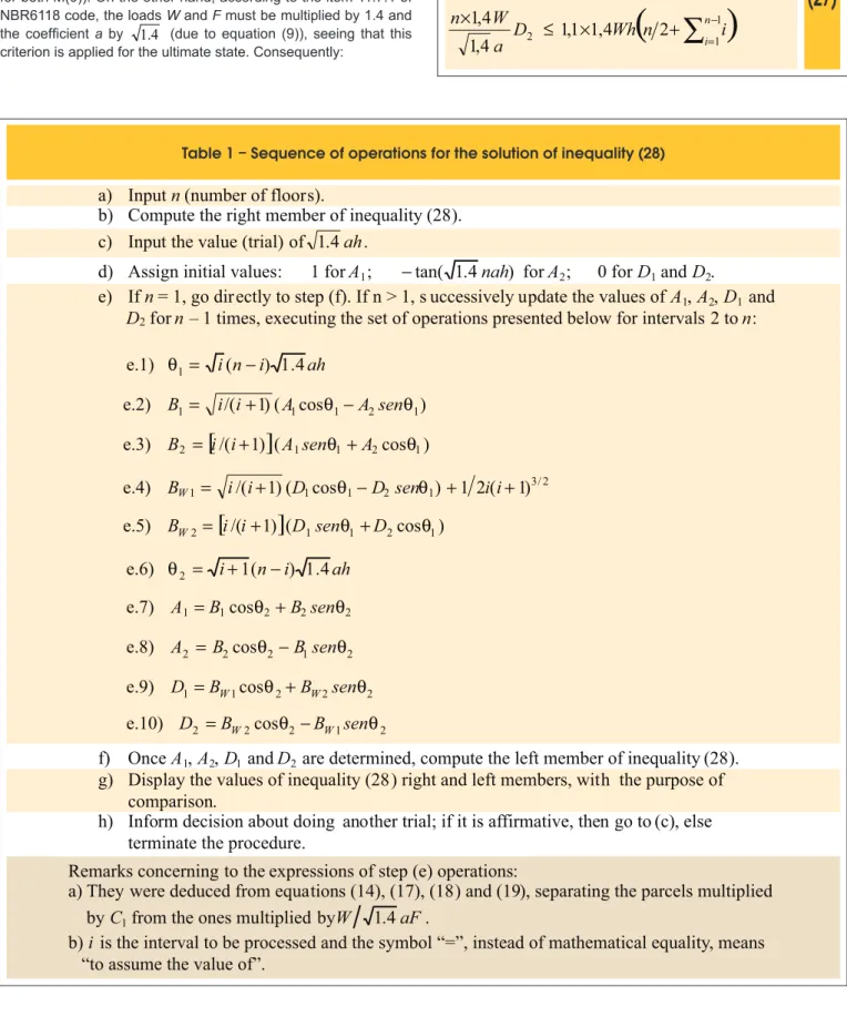
Table 1 – Sequence of operations for the solution of inequality (28)
a)
Input
n
(number of floors).
b)
Compute the right member of inequality (28).
c)
Input the value (trial) of
1
.
4
ah
.
d)
Assign initial values: 1 for
A
1;
-
tan(
1
.
4
nah
)
for
A
2; 0 for
D
1and
D
2.
e) If
n
= 1, go directly to step (f). If n > 1, s uccessively update the values of
A
1,
A
2,
D
1and
D
2for
n
– 1 times, executing the set of operations presented below for intervals 2 to
n
:
e.1)
q
1=
i
(
n
-
i
)
1
.
4
ah
e.2)
B
1=
i
/(
i
+
1
)
(
A
1cos
q
1-
A
2sen
q
1)
e.3)
B
2=
[
i
/(
i
+
1
)
]
(
A
1sen
q
1+
A
2cos
q
1)
e.4)
3/21 2 1 1
1
=
i
/(
i
+
1
)
(
D
cos
-
D
sen
)
+
1
2
i
(
i
+
1
)
B
Wq
q
e.5)
B
W2=
[
i
/(
i
+
1
)
]
(
D
1sen
q
1+
D
2cos
q
1)
e.6)
q
2=
i
+
1
(
n
-
i
)
1
.
4
ah
e.7)
A
1=
B
1cos
q
2+
B
2sen
q
2e.8)
A
2=
B
2cos
q
2-
B
1sen
q
2e.9)
D
1=
B
W1cos
q
2+
B
W2sen
q
2e.10)
D
2=
B
W2cos
q
2-
B
W1sen
q
2f)
Once
A
1,
A
2,
D
1and
D
2are determined, compute the left member of inequality (28).
g)
Display the values of inequality (28) right and left members, with the purpose of
comparison.
h)
Inform decision about doing another trial; if it is affirmative, then go to (c), else
terminate the procedure.
Remarks concerning to the expressions of step (e) operations:
a) They were deduced from equations (14), (17), (18) and (19), separating the parcels multiplied
by
C
1from the ones multiplied by
W
1
.
4
aF
.
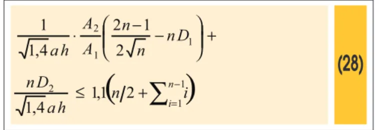
It is implied that the terms Α1, A2, D1 and D2 of equations (23) and (24) will have been obtained, applying equations (14), (17), (18)
and (19) with 1.4a in place of a. Performing the required alge
-braic transformations, inequality (27) changes into:
(28)
(
å
-)
=
+
£
11
2
,1
1
2
4
,
1
n i
i
n
h
a
D
n
+
÷÷ø
ö
ççè
æ
-
-×
11 2
2
1
2
4
,
1
1
n
D
n
n
A
A
h
a
For a small number of loors, it is feasible to derive expressions for Α1, A2, D1 and D2 as functions of
1
.
4
a
h
ah and then to replace theminto the left member of (28). Thereafter, inequality (28) can be solved by trials, obtaining the factor
1
.
4
a
h
ah. However, for a greater num-ber of loors, it is necessary to apply equations (18) and (19) many times, leading to very long expressions for Α1, A2 and consequently for the left member of (28). For buildings with more than four loors,
this method of determination of
1
.
4
a
h
ah becomes impracticable. In face of this circumstance, an alternative method was developed in or-der to determine the factor1
.
4
a
h
ah for buildings with a greater numberof loors. Through this method, the solution is also obtained by means of trials. However, instead of deducing longer and longer expressions for Α1, A2, D1 and D2, successive trials are done, assigning an initial value to
a
h
.
4
1
ah and determining numerical values for those variables. In eachtrial, the abovementioned formulary is applied in such a way to obtain numerical values for the right and left members of inequality (28). When
these values result close enough to be considered identical, then the factor
1
.
4
a
h
ah will have been determined.Due to the great quantity of calculations, the method is computer aid. With the purpose of illustration, table 1 shows the sequence of
operations for determining
1
.
4
a
h
ah by means of trials. Represent-ing by b the solution of inequality (28) obtained by this method and
considering a as expressed by equation (9), it may be written:
(29)
b
h
J
E
F
h
a
1
.
4
/
≤
4
.
1
=
It can be observed in igure 2 that h=Htot n andF=Nk n, with Nk as deined in subsection 1.2. On the other hand, since the wall or core behaves as a column, the physical nonlinearity may be considered,
substituting EJ by (EI)sec given by (6). This changes inequality (29) into:
(30)
4
.
1
≤
941
.
0
/
E
I
n
n
b
N
H
tot k CS COn comparing (30) with equations (3) and (4), it is concluded that
the limit α1 of the instability parameter may be expressed by:
(31)
2/ 3 1
=
b
n
0
.
941
n
1
.
4
=
0
.
82
b
n
a
Therefore, once the desired number of loors (n) is introduced into the
sequence of operations of table 1, the value of b can be determined; then, the value of the limit coeficient α1 can be obtained, applying equation (31). This was done for a series of loors quantities and the results are displayed in the second and ifth columns of table 2.
Table 2 – Values of
a
1 in function of the floors number (uniform wind load)
1
0.425
0.426
25
0.754
0.754
2
0.571
0.573
30
0.757
0.757
3
0.631
0.631
35
0.759
0.759
4
0.663
0.663
40
0.761
0.761
5
0.683
0.683
50
0.763
0.763
6
0.697
0.697
60
0.765
0.765
7
0.707
0.707
70
0.766
0.766
8
0.715
0.715
80
0.767
0.767
9
0.721
0.721
100
0.768
0.768
10
0.726
0.726
125
0.769
0.769
12
0.734
0.733
165
0.770
0.770
14
0.739
0.739
250
0.771
0.771
16
0.743
0.743
500
0.772
0.772
18
0.746
0.746
≥ 1100
0.773
0.773
20
0.749
0.749
–
–
–
n
a
1 (1)
a
1 (2)
n
a
1 (1)
a
1 (2)
3. The continuous model and the derivation
of an approximated formula for
α
1The values of α1, presented in table 2, may be considered as “ex
-act solutions” (in the context of the discrete model of igure 2) for the instability parameter limit of bracing systems composed ex
-clusively by walls and/or cores. Nevertheless, a question remains
unsolved, since the method developed in the preceding section
doesn’t provide an explicit formula for obtaining the limit coeficient α1. Thus, the aim of this section is to deduce approximated for -mulas that give the value of α1 in function of the number of loors with an adequate accuracy. At irst, the case of uniform wind load is considered; then, the case of wind load distributed according to NBR 6123 [7] prescriptions is treated.
It can be veriied that the continuous model, shown in igure 1-b, is inadequate for buildings with few loors. This is primarily because the simulation of a concentrated loads set by means of a distrib
-uted load only provides a good accuracy if the number of concen
-trated loads is large. In buildings with few loors, the model of igure 1-b fails mainly by no capturing the effect of the top vertical load. In order to avoid this drawback, the continuous model of igure 3,
with a vertical load P concentrated at the building top, is adopted.
3.1 Uniformly distributed wind load
If the distortions effect is neglected in the model of igure 3-a, it can
be proved that the linear solution, in terms of the rotations φ(x), for a uniform wind load of rate w, is given by:
(32)
ú
ú
û
ù
ê
ê
ë
é
÷
ø
ö
ç
è
æ
-=
3 3
1
1
6
)
(
x
EJ
w
x
f
Now, considering the distortions effect, the bending moments
func-tion will be expressed by:
(33)
[
]
ò
-x
q
y
(
x
)
y
(
x
)
d
x
[
-
]
-=
w
x
P
y
y
x
x
M
(
)
(
)
22
(
)
(
)
Representing by Y(x) the primitive function of the horizontal dis -placements y(x), equation (33) changes into:
(34)
[
(
)
(
)
]
2
)
(
)
(
x
w
x
2P
y
y
x
M
=
-
-
-
-[
Y
(
)
Y
(
x
)
(
x
)
y
(
x
)
]
q
-
-
--
Equating –EJ d 2y/dx2 to M(x) given by (34), leads to the differential
equation of motion. Deriving it in relation to x, remembering that dy/
dx = φ(x) and re-arranging, results:
(35)
0
)
(
)
(
)
(
/
2[
]
2
dx
+
P
+
q
-
x
x
+
w
-
x
=
d
J
E
f
f
In order to solve equation (35), Galerkin method will be adopted. It consists in obtaining an approximated solution of the form:
(36)
å
==
@
mi
a
i ix
x
x
)
(
)
1(
)
(
f
j
f
where ϕi(x) (i = 1, 2, . . ., m) are previously chosen functions
Figure 3 – Continuous model for the bracing system
Uniform wind load Wind load according to
NBR 6123 prescriptions
and the ai are coeficients to be determined. More detailed con
-siderations about Galerkin method can be seen in Kantorovitch and Krylov [8]. On applying the method for the actual case, the summation of equation (36) will be reduced to a single parcel
(m = 1) and a function proportional to the linear solution, given
by (32), will be adopted for ϕ1(x). Consequently, equation (36) changes into:
(37)
ú
ú
û
ù
ê
ê
ë
é
÷
ø
ö
ç
è
æ
-=
@
1 1(
)
11
1
3)
(
x
a
x
a
x
j
f
In order to obtain α1, the following equation must be solved:
(38)
[
]
ò
ïî
ï
í
ì
-+
+
•÷
ø
ö
ç
è
æ
-
0 2 1
)
(
1
6
EJ
a
x
P
q
x
=
ïþ
ï
ý
ü
-+
ú
ú
û
ù
ê
ê
ë
é
÷
ø
ö
ç
è
æ
--
1 31
1
1
x
w
(
x
)
(
x
)
dx
0
a
j
The term multiplied by ϕ1(x) is the differential operator regarding to
equation (35). Thus, introducing ϕ1(x) given by (37), performing the integration and isolating α1, gives:
(39)
3 2
3
1
6
(
15
/
7
)
(
3
/
4
)
q
P
EJ
w
a
-=
Replacing (39) into (37), leads to the function φ(x). Comparing it
with (32), it can be observed that the geometric nonlinearity arises
through the terms that are subtracted from 6EJ in the denomina-tor of α1. Integrating φ(x) twice, leads successively to the functions y(x) and Y(x). Substituting them into equation (34) and applying it for x = 0, leads to the following expression for the bending moment
at support:
(40)
3 2 3 2 2 27
20
56
)
2
5
(
5
7
2
)
0
(
q
P
EJ
q
P
w
w
M
-+
×
-=
In order to verify the exemption of second order effects con
-sideration, inequality (2) will be applied, replacing M II by the modulus of M(0) given by (40), with the loads multiplied by 1.4. Hence:
(41)
2
4
1
×
1
1
.
.
w
2≤
4
1
×
7
4
1
×
20
56
2
+
5
4
1
×
4
1
5
7
+
2
4
1
2 2 22 3 3
q
.
P
.
EJ
q
P
.
w
.
w
.
-)
(
Performing successive algebraic transformations, equation (41)
changes into:
(42)
2
≤
/
)
15
.
3
8
(
P
+
q
2EJ
The physical nonlinearity may be considered, substituting EJ by
(EI)sec given by (6). Then, extracting the square root of equation (42) both sides and re-arranging, gives:
(43)
773
.
0
≤
/
)
54
.
2
(
P
q
E
CSI
C
+
It must be remembered that the aim of this section is to obtain a formula for α1 in function of the number of loors. In order to do it starting from equation (43), it is necessary to ind a relation be -tween qℓ and P in function of the number of loors, in such a way
that the application of (43) provides α1 values as close to the ones presented in the second and ifth columns of table 2 as possible.
On the other hand, representing Htot by ℓ, equation (3) combined with (4) may be expressed as follows:
(44)
1a
£
C CSk
E
I
N
The factor ECS IC can be isolated in both equations (43) and (44). Then, equating the resulting expressions one another and
considering that the total vertical load Nk is given by the sum of P
and qℓ, it can be proved that:
(45)
2 1 2 2 2 1773
0
773
0
54
2
=
a
a
-.
.
.
P
q
The next step is to input the series of α1 values presented in table 2 (discrete model) into equation (45), determining successive values
for qℓ/P corresponding to successive loors quantities and listing them into table 3. Thereafter, an equation that provides values for
qℓ/P in function of n with an adequate accuracy must be searched. A possible solution consists of the following straight line equation:
(46)
528
1
201
1
=
.
n
.
P
q
-Finally, considering that ℓ is the height Htot and combining equa -tions (44), (45) and (46), results:
(47)
)
(
)
(
0
44
+
0
84
773
0
.
n
-
.
n
.
=
≤
1I
E
N
(50)
)
2
(
)
0
(
=
-
w
2p
+
M
T
On the other hand, considering the distortions effect and
fol-lowing the same deductive sequence that led to equations
(34) and (35), it can be proved that the bending moments
function and the differential equation of motion are respec
-tively given by:
(51)
[
y
(
)
y
(
x
)
] [
q
Y
(
)
Y
(
x
)
(
x
)
y
(
x
)
]
P
-
-
-
+
-)
2
)(
1
(
)
2
(
)
1
(
)
(
2 2
p
p
x
x
p
p
w
x
M
pp
T
+
+
-+
+
-+
×
-=
+
(52)
0
1
1=
+
-×
+p
x
w
T
p
p)
(
)
(
22
]
[
+
-
+
+
P
q
x
x
dx
d
EJ
f
f
In order to solve equation (52), Galerkin method will be used,
adopting a function ϕ1(x) proportional to the linear solution given
by (49). In the derivation proceeding, due to the great extension of the expressions that are generated, the formulary will be par
-ticularized for p = 0.35, which corresponds to a meteorological parameter p of 0.175, regarding to a terrain with category V
roughness. This value of p results in the most far from uniform distribution loading pattern. Thus, following the same deductive
sequence that led to equation (40), gives an expression for the In this way, an expression for α1 in function of the loors number
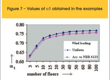
was obtained. Equation (47) was applied for the same series of loors numbers of table 2 and the resulting values are presented in its third and sixth columns. A quasi perfect coincidence between
the values of α1regarding to the discrete and continuous models
can be veriied; the respective graphs, shown in igure 4 for build
-ings ranging from 1 to 30 loors, appear superposed.
3.2 Wind load distributed according
to NBR 6123 prescriptions
Figure 3-b presents the model of a bracing system subject to a
wind load of rate w(x), variable along the height, reaching a value
wT = w(ℓ) on the building top. According to NBR 6123 (ABNT [7]) prescriptions, the rate w(x) may be expressed as follows:
(48)
p
x
K
x
w
(
)
=
(
/
10
)
K is a constant that depends on many factors, as: surface of the building face perpendicular to the wind direction; relation between the building dimensions; basic wind speed and topographic, statis
-tical and gust factors, as deined by NBR 6123. The exponent p is the double of the meteorological parameterp, varying from 0.06
until 0.175 and depending on the building dimensions and ground roughness. Thus, p can vary from 0.12 until 0.35.
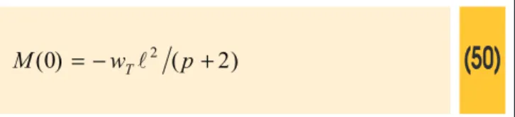
It can be proved that the rotations φ(x) and the support bending moment
M(0), due to irst order effects exclusively, are respectively given by:
(49)
)
2
)(
1
(
)
3
(
2
)
2
(
)
1
(
2 2 3+
+
+
+
+
-+
+p
p
x
x
p
p
x
p
p
p)
(
=
×
EJ
w
x
Tf
Table 3 – Values of q
ℓ
/P in function
of the floors number
Number
q
ℓ
/P
Number
q
ℓ
/P
of floors
of floors
1
-0.333
20
22.6
2
0.849
25
29.2
3
2.07
30
35.0
4
3.28
35
40.4
5
4.48
40
47.3
6
5.69
50
57.2
7
6.88
60
72.0
8
8.12
70
82.5
9
9.30
80
97.0
10
10.5
100
116
12
13.1
125
147
14
15.3
165
196
16
17.7
250
291
18
19.9
500
593
support bending moment including second order effects, as stat-ed below:
(53)
32 3 2 2
886
2
95
7
+
516
2
3505
0
q
P
.
EJ
.
q
P
.
w
.
T-)
(
2
4255
0
=
0
.
w
M
(
)
-
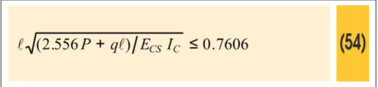
T-In order to verify the exemption of second order effects consider -ation, the moments M I and M II will be replaced by the modules of
M(0) respectively given by (50) and (53), with the loads multiplied by 1.4. In this way, applying inequality (2), replacing EJ by (EI)sec
given by (6) (physical nonlinearity) and performing the required
algebraic transformations, results:
(54)
7606
.
0
≤
)
556
.
2
(
P
q
E
CSI
C
+
Due to the similarity between equations (54) and (43), the same α1 variation pattern of uniform wind load will be assumed, with the coeficient 0.773 of (43) being changed to 0.7606. Consequently, an expression for α1 in function of the loors number, similar to equation (47), is obtained for wind load distributed according to
NBR 6123 prescriptions, as follows:
(55)
)
(
)
(
0
44
+
0
84
7606
0
.
n
-
.
n
.
=
≤
1I
E
N
H
tot k CS Ca
Isolating IC in equation (55), gives:
(56)
CStot k
C
.
n
n
.
.
N
E
H
I
≥
1
729
×
+
-
0
0
44
84
×
2Equation (56) is very useful in the preliminary stage of a bracing system design, especially when the aim is to obtain a ixed nodes structure, according to NBR 6118 deinition.
4. Examples
4.1 Description of the tests
The plan of igure 5 shows the basic coniguration of the transver
-sal bracing system of a building with an oblong octagonal shape on plane, being composed by walls 1 to 5. This system was employed in buildings having 3, 5, 10, 15, 20, 30 and 40 loors, constitut
-ing examples 1 to 7. In the same way, igure 6 shows the basic coniguration of the transversal bracing system composed by walls 1 to 7, which was employed in buildings with 50, 60, 80 and 100 loors, constituting examples 8 to 11. In examples 10 and 11, chan
-nel-shaped cores, indicated by the broken lines of igure 6, were utilized in place of walls 1 and 7.
In all the examples, it was adopted a story-height of 3 m, as well
as a concrete with fck = 25 MPa, resulting in an elasticity modu -lus ECS = 23800 MPa. A total vertical load of 10 kN/m2 per loor
(characteristic value) was considered. A wind pressure of 1.5 kN/
m2 (characteristic value), constant along the height, was initially
adopted, since it was an experience with a formulation based on a
model with constant wind load.
Each of the 11 bracing systems was tested, aiming to deter
-mine the relation between vertical loads and horizontal stiffness
that would result in a 10 % increase on the global moment at
building support, concerning to first order analysis; in this way,
the limit α1 for the instability parameter was determined. The
procedure applied in each test consisted in assigning initial di-mensions to the walls cross sections and performing a second
order analysis, employing the P-Delta method with double pre -cision processing. More detailed considerations about P-Delta
method can be seen in Smith and Coull [9]. After, this second order analysis was successively repeated, adjusting the cross
sections dimensions until achieve the desired 10 % increase
on the support global moment. The physical nonlinearity was
Figure 5 – Transversal bracing system:
examples 1 to 7
considered by means of the individual bars stiffness reduction, expressed by equation (6). Due to the bracing double symme
-try in plane, the analyses were performed using a plane frame model, with the walls joined among themselves by hinges rep -resenting the floor slabs.
Subsequently, the 11 examples were re-analyzed, considering a
along the height variable wind load. The NBR 6123 prescriptions were observed, considering the following parameters: basic wind
speed of 45 m/s; topographic and statistical factors equal to 1.0; and ground roughness of category V, corresponding to big cities
Table 4 – Results for uniform wind load
1
3
0.631
0.632
0.1226
5
20 x 114
2
5
0.683
0.684
0.4852
5
20 x 180
3
10
0.726
0.726
3.441
5
20 x 346
4
15
0.741
0.741
11.15
5
30 x 447
5
20
0.749
0.749
25.88
5
30 x 592
6
30
0.757
0.757
85.53
5
40 x 800
7
40
0.761
0.761
200.7
5
48 x 1000
8
50
0.763
0.763
1004
7
51 x 1500
9
60
0.765
0.765
1727
5
60 x 1771
–
–
–
–
–
+ 2
60 x 1500
10
80
0.767
0.767
4073
5
80 x 2000
–
–
–
–
–
+ 2
85 x 1500 (web) and 85 x 354 (edges)
11
100
0.768
0.768
7924
5
120 x 2200
–
–
–
–
–
+ 2
120 x 1500 (web) and 120 x 472 (edges)
4
Example
n
a
1 (1)
a
1 (2)
I (m )
CWalls
Cross section dimensions (cm)
n – floors number; a1 (1) – equation (47); a1 (2) – values obtained in the examples
centers. In order to estimate the initial dimensions of the walls
cross sections, equation (56) was applied.
4.2 Results discussion
The fourth column of table 4 shows the values of α1 found in the
11 examples, taking an uniform wind load into account. The follow -ing columns contain the values of the total gross inertia IC and the corresponding number of walls and cross section dimensions that led to the just mentioned values of α1. It can be observed that it
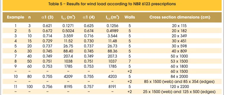
Table 5 – Results for wind load according to NBR 6123 prescriptions
1
3
0.621
0.1271
0.625
0.1256
5
20 x 115
2
5
0.672
0.5024
0.674
0.4989
5
20 x 182
3
10
0.714
3.559
0.716
3.544
5
20 x 349
4
15
0.729
11.52
0.730
11.48
5
30 x 451
5
20
0.737
26.75
0.737
26.73
5
30 x 598
6
30
0.745
88.40
0.745
88.36
5
40 x 809
7
40
0.749
207.4
0.749
207.3
5
50 x 1000
8
50
0.751
1038
0.751
1037
7
53 x 1500
9
60
0.753
1785
0.753
1785
5
60 x 1800
–
–
–
–
–
–
+2
60 x 1500
10
80
0.755
4209
0.755
4203
5
84 x 2000
–
–
–
–
–
–
+2
85 x 1500 (web) and 85 x 354 (edges)
11
100
0.756
8195
0.757
8191
5
120 x 2200
–
–
–
–
–
–
+2
25 x 1500 (web) and 125 x 500 (edges)
4 4