Key words: modal split, overland transport of general cargo, market share model, logistics costs, transport supply.
Palavras-Chave: divisão modal, transporte terrestre de carga geral, modelo de market share, custos logísticos, oferta de transporte.
Recommended Citation
* Email: [email protected].
Research Directory
Submitted 1 Feb 2013; received in revised form 13 Oct 2013; accepted 3 Nov 2013
Evaluating the modal split of overland transportation of
general cargo in Brazil using a market share model
[Avaliando a divisão modal do transporte terrestre de carga geral no Brasil usando um modelo de market share]
Federal University of Rio de Janeiro - Brazil, Federal University of Rio de Janeiro - Brazil, Federal University of Rio de Janeiro - Brazil, University of Brasília - Brazil
Resumo
O artigo apresenta metodologia desenvolvida para avaliar a divisão modal do transporte terrestre de carga geral no Brasil e possíveis razões para a prevalência do transporte rodoviário sob o transporte ferroviário, usando um modelo de market share. Não foram encontrados estudos que utilizaram o modelo de market share para o planejamento de transporte de carga, apesar de sua natureza genérica que permite que ele seja aplicado a qualquer mercado, serviço, utilidade ou produto. A metodologia foi aplicada em três corredores de transporte, dois grupos de carga geral e permitiu entender que as operações ferroviárias brasileiras continuam pouco competitivas em termos de custos logísticos para o transporte de carga geral de alto valor agregado. Além disso, constatou-se que a oferta de transporte é um fator determinante para o maior uso do transporte rodoviário na matriz de transporte de carga geral e que a demanda para o transporte de carga geral é elástica a esse fator. Para cargas de baixo valor agregado (VA1), a redução de 1% no gap entre oferta de transporte rodoviária e ferroviária leva a um aumento de 4,5% no market share ferroviário no CT1 (São Paulo - Porto Alegre - São Paulo), 4,9% no CT2 (Santos - Brasília - Santos) e 3,3% no CT3(São Paulo - Rio de Janeiro - São Paulo). Para cargas de alto valor agregado (VA2) a elasticidade foi mais intensa. A redução de 1% no gap entre oferta de transporte rodoviária e ferroviária leva a um aumento no market share ferroviário de 4,2% no CT1, 119% no CT2 e 9,6% no CT3.
Gonçalves, B., D'Agosto, M., Leal Jr., I. and Silva, F. (2014) Evaluating the modal split of overland transportation of general cargo in Brazil using a market share model. Journal of Transport Literature, vol. 8, n. 4, pp. 60-81.
Brunno Santos Gonçalves*, Márcio de Almeida D´Agosto, Ilton Curty Leal Jr., Francisco Gildemir Ferreira da Silva
Abstract
This paper presents a methodology developed to evaluate the modal split of land transport of general cargo in Brazil and possible reasons for the prevalence of road transport over rail, using a market share model. No studies were found using the market share model for planning cargo transport, in spite of its generic nature which makes it readily applicable to any market, service, utility or commodity. The methodology was applied in three transport corridors, two groups of general cargo and enabled us to establish that Brazilian rail operations are still uncompetitive in terms of logistics costs when transporting general cargo of high aggregate value. Moreover, transport supply is a determinant factor for the greater use of road transport in Brazil’s general cargo transport matrix, and the demand for general cargo transport in Brazil is elastic in relation to this factor. For low aggregate value general cargo (AV1), a 1% reduction in the gap between road and railway supply leads to an increase in the railway market share of 4.5% through TC1 (São Paulo - Porto Alegre - São Paulo), 4.9% through TC2 (Santos - Brasilia - Santos), and 3.3% through TC3(São Paulo - Rio de Janeiro - São Paulo). For high aggregate value general cargo (AV2), this elasticity was more pronounced. A 1% reduction in the gap between road and railway transport supply leads to an increase in the railway market share of 4.2% through TC1, 11.9% through TC2, and 9.6% through TC3.
ISSN 2238-1031
Introduction
This paper presents a methodology developed to evaluate the modal split of land transport of general cargo in Brazil and possible reasons for the prevalence of road transport over rail, using a market share model.
Using railways to transport general cargo1 in Brazil is still not a prevalent practice. Based on ANTT (2004), ANTT (2011) and ANTAQ (2010), the authors have estimated that railways transported a mere 7.9% of all Brazilian general cargo in 2011; approximately 25.5 million tons. In contrast, the more popular road transport mode accounted for 85.3% of cargo transportation in the same year; approximately 275.9 million tons.
Brazilian transport policy guidelines are attempting to establish a more equitable transport matrix with priority being given to the use of more economical and environmentally sustainable transport modes, particularly rail and waterway. The Brazilian government is therefore endeavoring to exploit the comparative advantages of different modes of transport and to integrate and combine their operations to achieve safer and more economical intermodal handling of goods.
Transport studies use various methodologies but new advances have been made in economics that can be useful for transport analysis. Train (2003) indicates that there are three kinds of approaches used in discrete choice models: disaggregate models, aggregate models and those using the dependent variable in the estimation process. The second approach is widely used in market economic structure analysis as, for example, in the works of Basuroy and Nguyen (1998), Nevo (2000) and Train (2003). No studies were found using Nevo’s (2000) approach, however, in spite of its generic nature which makes it readily applicable to any market, service, utility or commodity.
1
In this context, a methodology based on a market share model has been designed aimed at identifying and measuring factors that influence the greater use of road over rail transport in Brazil. The methodology is a useful tool for sector analysis and for planning cargo transport studies.
Section 1 presents the structured scientific methodology used for analysis, gaining an understanding of the problem and unfolding the research. Section 2 describes the study undertaken to analyze three important Brazilian transport corridors. In Section 3 there is a discussion of the results and lastly, the Section headed “Conclusions” presents the paper’s final remarks.
1. Methodology
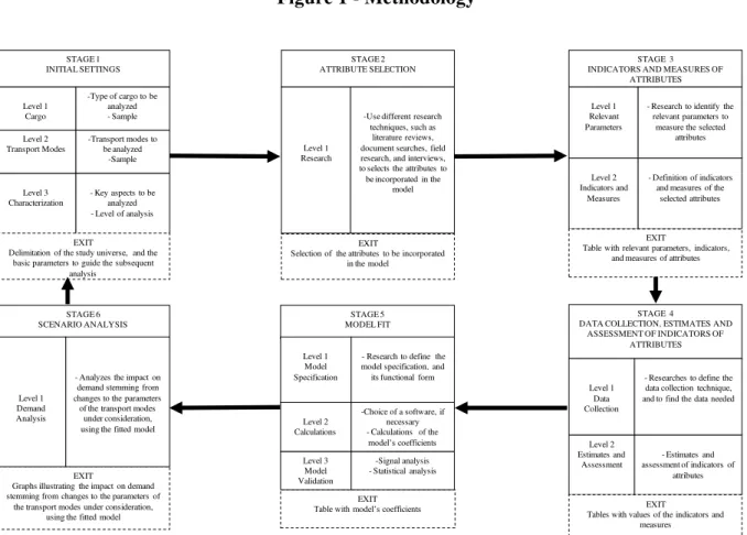
Figure 1 is a schematic illustration of the methodology. Details of the stages are set out in 2.1 to 2.6.
1.1 Stage 1 - Initial Settings
The initial settings in Stage 1 define the scope of the analysis, including the type of cargo and transport modes to be analyzed, a description of a representative sample, and a characterization of the analysis, including level and key aspects.
1.2 Stage 2 - Attribute Selection
Stage 2 selects the attributes to be incorporated to the model. They should reflect possible factors determining the use of the modes of transport under analysis and are investigated using research techniques such as literature reviews, document searches, field research, and interviews.
1.3 Stage 3 - Indicators and Attribute Measurement
Figure 1 - Methodology2
1.4 Stage 4 - Data Collection, Estimates, and Assessment of Attribute Indicators
In Stage 4 data is collected for assessing the attribute indicators. This information is necessary for the subsequent model fitting. The definition of the data collection technique takes into
account the availability of data and research resources. When it has been defined, the literature reviews and document searches to obtain the data needed to calculate the indicators
are completed. At this stage, the researcher can often come across gaps in the data and estimates are needed to continue the modeling.
Once data have been collected and/or estimated, the attribute indicator values and measurements determined in Stage 3 are calculated and assessed.
2
Source: Developed by the authors based on Leal Jr. and D’Agosto (2011). STAGE 1
INITIAL SETTINGS
Level 1 Cargo
-Type of cargo to be analyzed - Sample
Level 2 Transport Modes
-Transport modes to be analyzed
-Sample
Level 3 Characterization
- Key aspects to be analyzed - Level of analysis
EXIT
Delimitation of the study universe, and the basic parameters to guide the subsequent
analysis
STAGE 2 ATTRIBUTE SELECTION
Level 1 Research
-Use different research techniques, such as
literature reviews, document searches, field research, and interviews, to selects the attributes to be incorporated in the
model
EXIT
Selection of the attributes to be incorporated in the model
STAGE 3 INDICATORS AND MEASURES OF
ATTRIBUTES
Level 1 Relevant Parameters
- Research to identify the relevant parameters to
measure the selected attributes
Level 2 Indicators and
Measures
- Definition of indicators and measures of the
selected attributes
EXIT
Table with relevant parameters, indicators, and measures of attributes
STAGE 6 SCENARIO ANALYSIS
EXIT
Graphs illustrating the impact on demand stemming from changes to the parameters of
the transport modes under consideration, using the fitted model
STAGE 5 MODEL FIT
EXIT
Table with model’s coefficients
Level 1 Demand Analysis
- Analyzes the impact on demand stemming from changes to the parameters
of the transport modes under consideration, using the fitted model
Level 1 Model Specification
- Research to define the model specification, and its functional form
STAGE 4
DATA COLLECTION, ESTIMATES AND ASSESSMENT OF INDICATORS OF
ATTRIBUTES
Level 2 Estimates and
Assessment
- Estimates and assessment of indicators of
attributes
EXIT
Tables with values of the indicators and measures Level 3
Model Validation
-Signal analysis - Statistical analysis Level 2
Calculations
-Choice of a software, if necessary - Calculations of the
model’s coefficients
Level 1 Data Collection
1.5 Stage 5 - Model Fit
In Stage 5, the modeling technique, the model specification, and its functional form are first defined, and, if necessary, the appropriate software to fit the model is researched. The indicator values measured in Stage 4 provide the data for calculating the model’s coefficients.
With the model defined, the signs of the coefficients estimated for each variable are checked for theoretical consistency. Then, statistical analysis is performed to evaluate the significance level of both the model and the variables.
1.6 Stage 6 - Scenario Analysis
Stage 6 analyzes the impact on demand stemming from changes to the parameters of the
transport modes under consideration, using the fitted model. Changes in demand and the subsequent analysis are the result of a direct application of the model fitted in Stage 5.
Once Stage 6 is complete, the researcher may want to review the model, which is represented in the proposed procedure by means of a link between Stage 6 and Stage 1.
2. Methodology applied to a study
In sections 2.1 to 2.6, we apply the methodology illustrated in Figure 1.
2.1 Stage 1 - Initial Settings
During this stage, the scope of the Brazilian general cargo industry is analyzed with the aim of developing a model intended for the cargo transport strategic planner. The idea is to fit a modal split model that would consider the key attributes determining the choice between road and railway transport in Brazil, taking into account transfer operations between plants, ports, and distribution centers.
The demand for Brazilian general cargo allocated to the main transport corridors in the country was identified based on official data from the National Overland Transport Board (Agência Nacional de Transportes Terrestres) (ANTT, 2004). This demand was divided into
value (AV2). General cargo from the AV1 group has an average value of 25,000.00 R$/TEU3. The main products are construction supplies, steel products, and agricultural supplies. General cargo from the AV2 group has an average value of 75,000.00 R$/TEU. The main products are processed foods, beverages, electronics, home appliances, and automotive products.
For the subsequent analysis, the three transport corridors with the greatest flow of general cargo were selected: TC1 (São Paulo - Porto Alegre - São Paulo); TC2 (Santos - Brasilia - Santos); and TC3 (São Paulo - Rio de Janeiro - São Paulo). Figure 2 shows the three transport corridors which accounted for approximately 61.6% of the general cargo handled in Brazil in 2011.
Figure.2 - Selected transport corridors in Brazil4
TC1 has an average length of 1,100 km, connecting two highly industrialized regions of Brazil, the South and the Southeast. This corridor transported 81.8 million tons of general cargo in 2011(estimated by authors from ANTT, 2004), about 25.3% of the total cargo
handled that year.
3
TEU - twenty equivalent unit
4
Source: Developed by the authors.
TC3
TC2 has an average length of 700 km and is an important export and import corridor in Brazil. The corridor connects the state of São Paulo and the regions of Triângulo Mineiro and the Midwest to the Port of Santos. Moreover, it is the main route for the supply and distribution of the Brazilian wholesale industry concentrated in the region of Triângulo Mineiro. This corridor transported 53.0 million tons of general cargo in 2011(estimated by authors from ANTT, 2004), about 16.3% of the total cargo handled that year.
TC3, which has an average length of 430 km, connects the two largest Brazilian metropolitan areas, namely São Paulo and Rio de Janeiro. Moreover, it is an important transit route for cargo intended for the states of Minas Gerais and Espírito Santo, and for the northeastern and southern regions. This corridor transported 64.4 million tons of general cargo in 2011(estimated by authors from ANTT, 2004), about 19.9% of the total cargo handled that year.
Railways transported 10.0 million tons of general cargo through these three transport corridors in 2011 (ANTT, 2011); approximately 39.3% of the total Brazilian general cargo moved by rail in that year. The rail cargo in the three corridors was subdivided as follows: 3.2 million tons through TC1; 3.9 million tons through TC2; and 2.9 million tons through TC3. The cargo transported in these corridors was mainly general cargo of low aggregate value (7.7 million tons) and non-containerized general cargo (8.8 million tons).
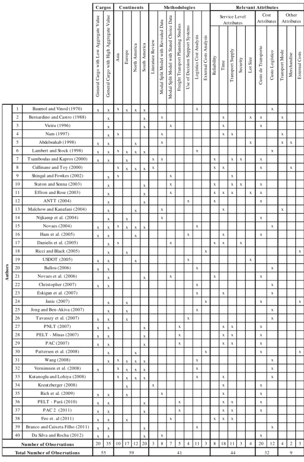
2.2 Stage 2 - Attribute Selection
Table 1 - Literature review5
5
Source: Developed by the authors.
R el ia b il it y T im e T ra n sp o rt S u p p ly S ec u ri ty L o t S iz e C u st o d e T ra n sp o rt e C u st o L o g ís ti co T ra n sp o rt M o d e M er ch an d is e E x te rn al C o st s
1 Baumol and Vinod (1970) x x x x x x x x 2 Bernardino and Castro (1988) x x x x x x x
3 Vieira (1996) x x x x x
4 Nam (1997) x x x x x x
5 Abdelwahab (1998) x x x x x x x
6 Lambert and Stock (1998) x x x x x x x x 7 T samboulas and Kapros (2000) x x x x x x x x x
8 Cullinane and T oy (2000) x x x x x x x x x 9 Shingal and Fowkes (2002) x x x x
10 Staton and Senna (2003) x x x x x x x 11 Effron and Rose (2003) x x x x x x x x
12 ANT T (2004) x x x x x
13 Malchow and Kanafani (2004) x x x x x
14 Nijkamp et al. (2004) x x x x
15 Novaes (2004) x x x x x x x x
16 Ham et al. (2005) x x x x x x
17 Danielis et al. (2005) x x x x x x
18 Ricci and Black (2005) x x x x
19 USDOT (2005) x x x x x
20 Ballou (2006) x x x x
21 Novaes et al. (2006) x x x x x
22 Christopher (2007) x x x x
23 Eskigun et al. (2007) x x x
24 Janic (2007) x x x x x
25 Jong and Ben-Akiva (2007) x x x x
26 T avasszy et al. (2007) x x x x x
27 PNLT (2007) x x x x x x x
28 PELT - Minas (2007) x x x x x x x
29 PAC (2007) x x x x x x x
30 Pattersen et al. (2008) x x x x x
31 Wang (2008) x x x x x x x
32 Vernimnen et al. (2008) x x x x x x x 33 Kutanoglu and Lohiya (2008) x x x x x x x
34 Kreutzberger (2008) x x x x
35 Rich et al. (2009) x x x x x x
36 PELT - Pará (2010) x x x x x x x
37 PAC 2 (2011) x x x x x x x
38 Feo et. al (2011) x x x x x x x
39 Branco and Caixeta Filho (2011) x x x x x 40 Da Silva and Rocha (2012) x x x x x
20 35 10 17 12 20 3 8 7 5 4 11 3 8 18 11 3 4 20 12 4 2 3
S o u th A m er ic a L it er at u re R ev ie w
C argos C ontine nts Me thodologie s Re le vant Attribute s
F re ig h t T ra n sp o rt P la n n in g S tu d ie s L o g is ti cs C o st A n al y si s Other Attributes A u th o rs
Numbe r of O bse rvations
Total Numbe r of O bse rvations 55 59
M o d al S p li t M o d el w it h R ev ea le d D at a A si a E u ro p e N o rt h A m er ic a G en er al C ar g o w it h L o w A g g re g at e V al u e G en er al C ar g o w it h H ig h A g g re g at e V al u e
44 32 9
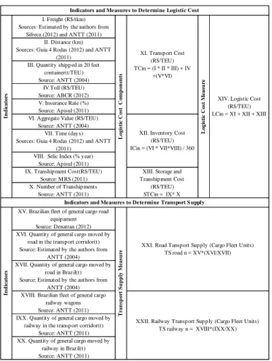
2.3 Stage 3 - Attribute Indicators and Measurements
The Table 2 shows indicators and measurements used to determine the time series of logistics costs and the levels of road and railway transport supply on the selected transport corridors. The measurement of logistics costs was taken to be the sum of the transport, stock, handling, and storage costs between a source and a destination, as proposed by Baumol and Vinod (1970). To measure transport supply, we assumed that the supply of both road and railway transport for general cargo in a specific transport corridor is proportional to the amount of general cargo handled by the transport mode in the corridor in question.
Table 2 - Indicators and measures to determine logistics costs and transport supply6
2.4 Stage 4 - Data Collection, Estimates and Assessment of Attribute Indicators
During this stage, we collected the required data, representing logistics operations already
performed for the transport of general cargo. Table 3 also shows the sources used to gather
6
Source: Developed by the authors.
I. Freight (R$/tkm) Sources: Estimated by the authors from
Sifreca (2012) and ANTT (2011) II. Distance (km) Sources: Guia 4 Rodas (2012) and ANTT
(2011) III. Quantity shipped in 20 feet
container(t/TEU) Source: ANTT (2004)
IV.Toll (R$/TEU) Source: ABCR (2012) V. Insurance Rate (%) Source: Apisul (2011) VI. Aggregate Value (R$/TEU)
Source: ANTT (2004) VII. Time (days) Sources: Guia 4 Rodas (2012) and ANTT
(2011)
VIII. Selic Index (% year) Source: Apisul (2011) IX. Transhipment Cost(R$/TEU)
Source: M RS (2011) X. Number of Transhipments
Source: ANTT (2011)
XV. Brazilian fleet of general cargo road equipament Source: Denatran (2012) XVI. Quantity of general cargo moved by
road in the transport corridor(t) Source: Estimated by the authors from
ANTT (2004) XVII. Quantity of general cargo moved by
road in Brazil(t) Source: Estimated by the authors from
ANTT (2004) XVIII. Brazilian fleet of general cargo
railway wagons Source: ANTT (2011) IXX. Quantity of general cargo moved by
railway in the transport corridor(t) Source: ANTT (2011) XX. Quantity of general cargo moved by
railway in Brazil(t) Source: ANTT (2011)
Indicators and Measures to Determine Transport S upply
In d ic ato rs Tr an sp or t S u p p ly M eas u re
XXI. Road Tansport Supply (Cargo Fleet Units) TS road n = XV*(XVI/XVII)
XXII. Railway Transport Supply (Cargo Fleet Units) TS railway n = XVIII*(IXX/XX) Indicators and Measures to Determine Logistic Cost
In d ic ato rs Lo gi sti c C os
t C
omp
on
en
ts
XI. Transport Cost (R$/TEU) TCin = (I * II * III) + IV
+(V*VI) Lo gi sti c C os t M eas u re
XIV. Logistic Cost (R$/TEU) LCin = XI + XII + XIII
XII. Inventory Cost (R$/TEU) ICin = (VI * VII*VIII) / 360
XIII. Storage and Transhipment Cost
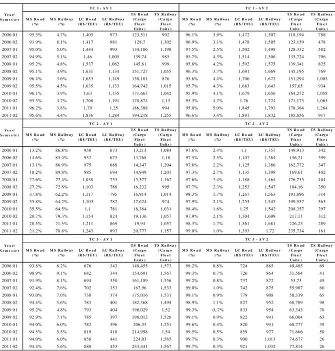
information about the indicators used to calculate the time series of market share, logistics costs and transport supply statistics. From this collected data, it was possible to estimate and assess the indicators of the selected attributes, thereby creating the database we required to fit the modal split models. This database contained biannual time series of road and railway, market share, logistics costs, and transport supply data.
Table 3 - Database for the fitting of modal split models7
7
Legend: TC1 - Transport Corridor 1; TC2 - Transport Corridor 2; TC3 - Transport Corridor 3; MS Road - Road Market Share; MS Railway - Rail Market Share; LC Road - Road Logistics Cost; LC Railway - Rail Logistics Cost; TS Road - Road Transport Supply; TS Railway - Rail Transport Supply. Source: Developed by the authors.
M S R o a d ( %)
M S R a ilwa y ( %)
LC R o a d ( R $ / T E U)
LC R a ilwa y ( R $ / T E U)
T S R o a d ( C a rg o
F le e t Un it s )
T S R a ilwa y ( C a rg o
F le e t Un it s )
M S R o a d ( %)
M S R a ilwa y ( %)
LC R o a d ( R $ / T E U)
LC R a ilwa y ( R $ / T E U)
T S R o a d ( C a rg o
F le e t Un it s )
T S R a ilwa y ( C a rg o
F le e t Un it s )
2006 01 95.3% 4.7% 1,405 973 123,511 992 96.1% 3.9% 1,472 1,507 118,194 788
2006 02 91.9% 8.1% 1,417 981 128,7 1,302 96.9% 3.1% 1,478 1,505 123,159 478
2007 01 95.0% 5.0% 1,444 993 134,106 1,198 97.5% 2.5% 1,502 1,498 128,332 582
2007 02 94.9% 5.1% 1,46 1,005 139,74 985 95.7% 4.3% 1,514 1,506 133,724 796
2008 01 95.2% 4.8% 1,537 1,062 145,61 999 95.8% 4.2% 1,592 1,575 139,341 825
2008 02 95.1% 4.9% 1,631 1,134 151,727 1,055 96.3% 3.7% 1,691 1,669 145,195 769
2009 01 96.4% 3.6% 1,653 1,149 158,101 876 95.6% 4.4% 1,706 1,672 151,294 1,005
2009 02 95.5% 4.5% 1,635 1,133 164,742 1,015 95.7% 4.3% 1,683 1,643 157,65 934
2010 01 96.1% 3.9% 1,63 1,135 171,663 1,042 95.9% 4.1% 1,679 1,656 164,272 1,058
2010 02 95.3% 4.7% 1,708 1,191 178,874 1,13 95.3% 4.7% 1,76 1,724 171,173 1,065
2011 01 96.2% 3.8% 1,79 1,25 186,388 994 95.0% 5.0% 1,845 1,793 178,364 1,264
2011 02 95.6% 4.4% 1,836 1,284 194,218 1,255 96.6% 3.4% 1,891 1,832 185,856 917
M S R o a d ( %)
M S R a ilwa y ( %)
LC R o a d ( R $ / T E U)
LC R a ilwa y ( R $ / T E U)
T S R o a d ( C a rg o
F le e t Un it s )
T S R a ilwa y ( C a rg o
F le e t Un it s )
M S R o a d ( %)
M S R a ilwa y ( %)
LC R o a d ( R $ / T E U)
LC R a ilwa y ( R $ / T E U)
T S R o a d ( C a rg o
F le e t Un it s )
T S R a ilwa y ( C a rg o
F le e t Un it s )
2006 01 13.2% 86.8% 950 673 13,213 1,084 97.6% 2.4% 1,1 1,357 149,913 342
2006 02 14.6% 85.4% 957 675 13,768 1,18 97.5% 2.5% 1,107 1,364 156,21 399
2007 01 13.1% 86.9% 975 688 14,347 1,204 97.8% 2.2% 1,125 1,386 162,772 347
2007 02 10.2% 89.8% 985 694 14,949 1,201 97.3% 2.7% 1,135 1,398 169,61 402
2008 01 22.6% 77.4% 1,038 735 15,577 1,162 97.6% 2.4% 1,188 1,464 176,735 404
2008 02 27.2% 72.8% 1,103 788 16,232 995 97.7% 2.3% 1,253 1,547 184,16 350
2009 01 37.8% 62.2% 1,117 795 16,914 1,014 98.3% 1.7% 1,267 1,563 191,896 314
2009 02 35.8% 64.2% 1,103 782 17,624 974 97.9% 2.1% 1,253 1,545 199,957 363
2010 01 35.5% 64.5% 1,1 781 18,364 1,031 98.4% 1.6% 1,25 1,542 208,357 297
2010 02 20.7% 79.3% 1,154 824 19,136 1,057 97.9% 2.1% 1,304 1,609 217,11 312
2011 01 28.5% 71.5% 1,211 869 19,94 1,057 98.3% 1.7% 1,361 1,681 226,23 289
2011 02 21.2% 78.8% 1,243 893 20,777 1,157 99.0% 1.0% 1,393 1,72 235,734 161
M S R o a d ( %)
M S R a ilwa y ( %)
LC R o a d ( R $ / T E U)
LC R a ilwa y ( R $ / T E U)
T S R o a d ( C a rg o
F le e t Un it s )
T S R a ilwa y ( C a rg o
F le e t Un it s )
M S R o a d ( %)
M S R a ilwa y ( %)
LC R o a d ( R $ / T E U)
LC R a ilwa y ( R $ / T E U)
T S R o a d ( C a rg o
F le e t Un it s )
T S R a ilwa y ( C a rg o
F le e t Un it s )
2006 01 93.8% 6.2% 676 343 148,455 1,573 99.2% 0.8% 724 865 49,485 69
2006 02 90.9% 9.1% 682 344 154,691 1,567 99.3% 0.7% 726 864 51,564 41
2007 01 91.9% 8.1% 694 350 161,189 1,556 99.2% 0.8% 737 872 53,73 49
2007 02 92.4% 7.6% 702 353 167,96 1,533 99.0% 1.0% 742 875 55,987 66
2008 01 93.0% 7.0% 738 374 175,016 1,531 99.1% 0.9% 779 908 58,339 65
2008 02 94.4% 5.6% 783 401 182,368 1,494 98.9% 1.1% 827 952 60,789 98
2009 01 95.2% 4.8% 793 404 190,029 1,52 99.3% 0,.7% 833 954 63,343 70
2009 02 92.9% 7.1% 785 397 198,012 1,526 99.1% 0.9% 822 941 66,004 63
2010 01 94.0% 6.0% 782 396 206,33 1,551 99.6% 0.4% 820 941 68,777 39
2010 02 94.5% 5.5% 819 418 214,998 1,54 99.5% 0.5% 859 977 71,666 50
2011 01 94.0% 6.0% 858 441 224,03 1,565 99.7% 0.3% 900 1,013 74,677 26
2011 02 94.4% 5.6% 880 453 233,441 1,567 99.7% 0.3% 921 1,032 77,814 26
Ye a r/ S e m e s t e r
T C 3 - A V 1 T C 3 - A V 2
Ye a r/ S e m e s t e r
T C 2 - A V 1 T C 2 - A V 2
Ye a r/ S e m e s t e r
2.5 Stage 5 - Model Fit
Logit Multinominal Modelling - MLM (Equation 1) and variations of it like the Probit Model (Equation 2) were used, both widely diffused and accepted in the academic and transport planning researches as, for example, in the works of Vassallo (2010), Oliveira (2010), Da
Silva and De Souza (2013) and Maitra et al. (2013).
N
k U U
i
j i
e e P
0
Where Pi = Probability of alternative i being selected; Ui = Utility of alternative i; Uj =
Utility of the j alternatives considered; e = Neper number ( 2.78182); N = number of alternatives considered.
Where Pi = Probability of alternative i being selected; Ui = Utility of alternative i; e = Neper number. The database needed to fit the modal split models can be taken from observational data, the so-called Revealed Preference data or from behavioral research survey data (Declared Preference). According to the type of data, different econometric techniques are used to adjust the utility function coefficients of the modal split model. Models based on Revealed Preference data are usually adjusted using the Ordinary Least Squares method while modal split models based on Declared Preference are adjusted using the Maximum Likelihood technique. Special softwares are available for applying the respective methods.
The market share model, adapted from the researches works of Basuroy and Nguyen (1998), Nevo (2000), and Train (2003), was chosen to fit the modal split models for each of the selected transport corridors and groups of general cargo. As Nevo (2000) has shown, the market share model is developed from an adaptation of logit-type models, assuming that the probability of choosing a transport alternative is equal to the market share of that alternative. Thus, the market share of an alternative is given by Equation 3.
(1)
i
U i
e
1
1
P
N 20 k
U U
i
j i
e
e
MS
(3)
Where MSi = Market Share of alternative i; Ui = Utility of alternative i; Uj = Utility of alternative j; e = Neper number; N = Number of alternatives. By transforming Equation 1 into its log-linear form, we obtain Equation 4.
lnMSi lnMSj Ui Uj (4)
Adapting Equation 2 to the model developed for the analysis of handling of general cargo in Brazil, as proposed in this paper, we obtain Equation 5.
lnMSRkjt lnMSFkjt β0 β1(LCRkjt LCFkjt ) β2(TSRkjt TSFkjt) (5)
Where MSRkjt = Market share of the road alternative in transport corridor k, for the transport of general cargo of aggregate value j in semester t; MSFkjt = Market share of the rail alternative in transport corridor k, for the transport of general cargo of aggregate value j in semester t; LCRkjt = Logistics costs of the road alternative in transport corridor k, for the transport of general cargo of aggregate value j in semester t (R$/TEU); LCFkjt = Logistics costs of the rail alternative in transport corridor k, for the transport of general cargo of aggregate value j in semester t (R$/TEU); TSRkjt =Transport supply of the road alternative in transport corridor k, for the transport of general cargo of aggregate value j in semester t (cargo fleet units); TSFkjt =Transport supply of the rail alternative in transport corridor k, for the
transport of general cargo of aggregate value j in semester t (cargo fleet units); 1,2 =
Coefficients; 0= Constant.
The time series data shown in Table 3 was used with the GRETL® software to fit the market share model for each transport corridor and general cargo group.
2.6 Stage 6 - Scenario Analysis
transport market share for a hypothetical situation resulting from changes in the values of the explanatory variables of the model.
The calculation of the rail transport market share was performed based on Equation 5, considering that the sum of the rail and road market shares is 100% (Equation 6). From these
two equations, we obtained Equation 7, which determines the rail transport market share of a given transport corridor.
MSRkjt MSFkjt 1 (6)
1
1
MS
e
β β (LC LC ) β (TS TS )Fkjt 0 1 Rkjt Fkjt 2 Rkln Fkjt
(7)3. Results and Discussion
An analysis of the results obtained at each stage of the applied procedure showed that the handling of general cargo in Brazil is heavily concentrated in the southern and southeastern regions of the country. As a result, the three analyzed transport corridors (results from Stage 1) handle 61.6% of the total cargo transported. An analysis of the general cargo transported through these corridors by rail showed that the average aggregate value and the level of containerization of these cargos are both low, suggesting that rail logistics costs and rail transport supply are still uncompetitive for goods with higher aggregate value.
The literature review detailed in Table 1 shows that these authors agree with the selection of attributes used to model the modal choice, usually selecting the attributes of cost and service
level. However, there is no consensus regarding the most suitable indicators to measure these two attributes. An analysis of the problem proposed in this paper suggests that logistics costs and transport supply are adequate indicators, although, in fact, only transport supply has shown satisfactory statistical results.
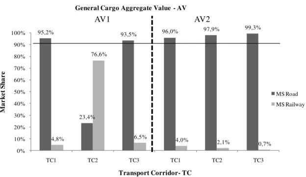
The average market share analysis of road and rail operations for general cargo categories, during the observation period (Figure 3), showed that, with the exception of low aggregate value general cargo through TC2, the remaining transport corridors have a road market share above 90%. This confirms the greater tendency to use road transport for general cargo in the
country. The average rail transport market share of 76.6% through TC2 for the transportation of general cargo in the AV1 category shows that a significant amount of agricultural and
construction supplies is transported by rail through this particular corridor.
Figure 3 - Market share in transport corridors8
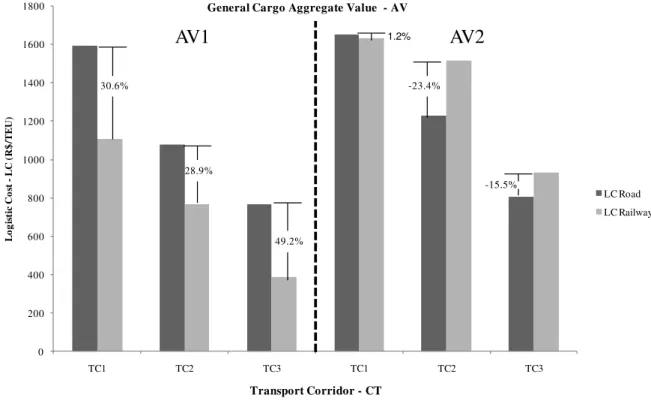
An analysis of the average logistics costs of road and rail operations for general cargo categories during the observation period (Figure 4) showed that, for the three transport corridors analyzed, rail logistics costs are competitive when transporting general cargo of low aggregate value (AV1). This finding reflects the fact that some Brazilian rail operations have been designed for door-to-door delivery of these cargo categories, with railway branch lines connecting factories to storage centers, thereby avoiding any additional cargo transfer or road transport costs.
For the high aggregate value general cargo group (AV2), rail transport has a small competitive advantage in terms of logistics costs, but only through TC2, where the average
8
Source: Developed by the authors.
95,2%
23,4%
93,5% 96,0% 97,9%
99,3%
4,8%
76,6%
6,5% 4,0%
2,1% 0,7% 0%
10% 20% 30% 40% 50% 60% 70% 80% 90% 100%
TC1 TC2 TC3 TC1 TC2 TC3
M
a
rk
et
S
h
a
re
Transport Corridor- TC
Market Share in Transport Corridors by Group of General Cargo
General Cargo Aggregate Value - AV
MS Road MS Railway
logistics costs of road-railway intermodal operations is 1.2% lower than the unimodal road operation. This advantage reflects the competitiveness of rail freight for average distances above 600 km, as is the case in this transport corridor. In contrast, the transport figures for these cargos through TC2 and TC3 show that road-railway intermodal transport is still
uncompetitive in them. This finding reflects a scenario in which railway fares are still uncompetitive when compared to road freight charges and, furthermore, there are additional
cargo transfer and road transport costs associated to the rail operations.
Figure 4 - Comparison of logistics costs9
An analysis of the transport supply side (Figure 5) showed that the supply of road transport for general cargo in Brazil has been growing steadily over time, being historically much more significant than the supply of rail transport for this type of cargo which has remained virtually unchanged. As a result, the gap between road and rail transport supply, which was approximately 598,000 cargo fleet units in the first half of 2006, has been gradually growing, reaching 942,700 cargo fleet units in 2011. This represents an increase of 53.6% during this period. These findings, highlighting the gap between road and rail transport supply, explain the predominance of road transport for general cargo in Brazil.
0 200 400 600 800 1000 1200 1400 1600 1800
TC1 TC2 TC3 TC1 TC2 TC3
L
o
g
is
ti
c
C
o
st
-L
C
(
R
$
/T
E
U
)
Transport Corridor - CT General Cargo Aggregate Value - AV
LC Road
LC Railway 30.6%
28.9%
49.2%
-23.4%
-15.5%
1.2%
Figure 5 - Evolution of road and railway transport supply
in the analyzed transport corridors10
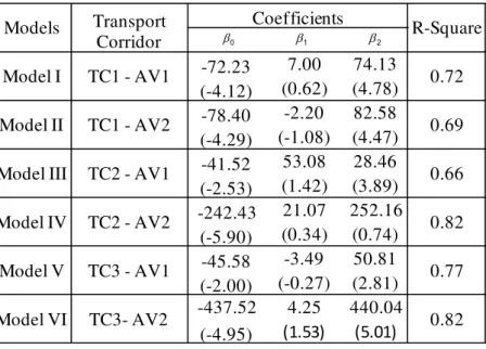
An analysis of the fitted models (Table 4) shows that all six models had an adjusted R-Square value above 0.60. An analysis of the coefficients of the logistics costs variable (�1) showed
that these reached a significance level above 90%, but only for Models III and VI. However, in these models, these coefficients were positive, which is inconsistent with the expected result that the logistics costs variable would be inversely proportional to the market share variable. This may reflect the fact that general cargo demand was evaluated in an aggregated manner, segmented into two groups of general cargo only. Furthermore, the results may be a reflection of the sample size, the lack of data variability and the existence of endogenous variables that were not incorporated to the modeling. Thus, the data analysis performed in Stage 4 did not consider points where there is a migration of general cargo from road to rail as a result of decreases in railway logistics costs.
An analysis of the coefficients of the transport supply variable (�2) showed that these attained statistical significance for all six fitted models. Moreover, in all the models, these coefficients were positive, which is consistent with the expected result that the transport supply variable would be directly proportional to the market share variable. These results show that the
10
Source: Ibidem.
602,8 628,1
654,5 682,0
710,6 740,5
771,6 804,0
837,8 873,0
909,6 947,8
4,8 5,0 4,9 5,0 5,0 4,8 4,8 4,9 5,0 5,2 5,2 5,1
0 500 1000
2006 01 2006 02 2007 01 2007 02 2008 01 2008 02 2009 01 2009 02 2010 01 2010 02 2011 01 2011 02
T
ra
n
sp
or
tS
u
p
pl
y
–
TS
(T
h
o
u
sa
nd
s
of
C
ar
go
F
le
et
U
n
it
s)
Year/Semester
Transport Supply Evolution
TS Road TS Railway 598.0
transport supply variable was the key explanatory variable in the fitted models, reflecting the fact that the largest market share for the road transport of general cargo is highly correlated to the large supply of road transport and low supply of railway transport for this market niche.
Table 4 - Statistical results of fitted model11
In Stage 6, we analyzed the changes in the rail transport market share relative to the transport
supply variable.12 To perform this analysis, the gap between road and rail transport supply was reduced by 1% in each of the analyzed transport corridors by assuming that the road transport fleet has remained unchanged since the second half of 2011. Changes in the rail transport market share thus obtained are shown in Figure 6.
The analysis shows that for both low aggregate value (AV1) and high aggregate value (AV2) general cargo, demand was elastic relative to fluctuations in the values of the transport supply variable.
For low aggregate value general cargo (AV1), a 1% reduction in the gap between road and railway supply leads to an increase in the railway market share of 4.5% through TC1, 4.9% through TC2, and 3.3% through TC3. For high aggregate value general cargo (AV2), this elasticity was more pronounced. A 1% reduction in the gap between road and railway transport supply leads to an increase in the railway market share of 4.2% through TC1, 11.9% through TC2, and 9.6% through TC3.
11
Legend: Numbers in brackets represent t-student values.� - constant; � - coefficient of variable Logistics costs; � - coefficient of variable Transport supply. Source: Developed by the authors.
12
Scenario analysis addressing changes in logistics costs were not performed because this variable’s coefficient
Models Transport Corridor
Coefficients
R-Square
Model I TC1 - AV1 -72.23 7.00 74.13 0.72 (-4.12) (0.62) (4.78)
Model II TC1 - AV2 -78.40 -2.20 82.58 0.69 (-4.29) (-1.08) (4.47)
Model III TC2 - AV1 -41.52 53.08 28.46 0.66 (-2.53) (1.42) (3.89)
Model IV TC2 - AV2 -242.43 21.07 252.16 0.82 (-5.90) (0.34) (0.74)
Model V TC3 - AV1 -45.58 -3.49 50.81 0.77 (-2.00) (-0.27) (2.81)
Model VI TC3- AV2 -437.52 4.25 440.04 0.82 (-4.95) (1.53) (5.01)
0
Results show that TC2 is the most attractive corridor for both AV1 and AV2 cargos. For rail transport of the AV1 group, TC2 can potentially increase by 508 tons per cargo fleet unit. For rail transport of the AV2 group, TC2 can potentially increase by 985 tons per cargo fleet unit. These numbers may reflect the high potential of rail transport of general cargo in the AV2
category through TC2.
TC1 has a similar attractiveness for both AV1 and AV2 cargos, with potential to increase by
447 tons per car for AV1 group cargos and 408 tons per car for AVA2 group cargos, respectively. These numbers may stem from the fact that the railway supply for both AV1 and AV2 groups through TC2 are very similar.
TC3 is the least attractive for rail transport of the AV1 group with potential to increase by 357 tons per cargo fleet unit only. However, for AV2 cargos, TC3, as in TC2, is very attractive. Here, TC3 could potentially increase by 843 tons per cargo fleet unit. This number may also reflect the high potential for the rail transport of general cargo from the AV2 group through TC3.
Figure 6 - Sensitivity of transport supply13
13
Source: Developed by the authors.
(4.5%; 447 t/cargo fleet unit) (4.2%; 408 t/cargo fleet unit) (4.9%; 508 t/ cargo fleet
unit)
(11.7%; 985 t/cargo fleet unit)
(3.3%; 357 t/cargo fleet unit)
(9.6%; 843 t/cargo fleet unit)
0% 2% 4% 6% 8% 10% 12% 14%
Simulated Situation AV1
Reference Date 2011 02
Simulated Situation AV2
R
a
il
w
a
y
M
a
rk
et
S
h
a
re
V
a
ri
a
ti
o
n
Sensitivity of Transport Supply
TC1
TC2
Conclusion
The aim of this paper was to evaluate the modal split of land transport of general cargo in Brazil and possible reasons for the prevalence of road transport over rail transport, using a market share model.
Applying the methodology developed in this study has provided an insight into the land transport of general cargo in Brazil, providing a unique and novel portrait of the recent behavior of demand, logistics costs, and transport supply for this market niche.
Results have shown that the preferential use of road transport, to the detriment of rail transport, for general cargo in Brazil is due to the low competitiveness of the railways in terms of logistics costs for transporting general cargo of higher aggregate value, which leads us to suggest that Brazilian railways are not yet ready for the large-scale transportation of such goods.
In addition, another determining factor for this road transport predominance is the existence of a growing supply of road transport in contrast to the small and virtually unchanged supply of rail transport. Based on the supply elasticity analysis, this scenario is likely to change, should the rail transport supply in Brazil come to be stimulated and promoted.
The major limitations of the developed model were the unavailability of time series data concerning the handling of general cargo on Brazilian roads and railways prior to 2006, and the lack of demand data classified according to a wider range of goods categories. These limitations precluded a more disaggregated analysis of the goods that are part of the scope of general cargo in Brazil.
References
ABCR (2012) Concessionárias. Work Document - ABCR (consulted in www.abcr.org.br).
Abdelahab, W. M. (1998) Elasticities of mode choice probabilities and market elasticities of demand: evidence from simultaneous mode choice/shipment-size freight transport model. Transportation Research E, 34, n. 4, pp. 257-266.
ANTAQ (2010) Navegação de Interior - Estatística 2010. Work Document - ANTAQ (consulted in www.antaq.gov.br).
ANTT (2004) Logística e Transporte para Produtos de Alto Valor Agregado no Contexto Brasileiro.
Work Document - ANTT (unpublished study).
ANTT (2011) SAFF - Sistema de Acompanhamento Ferroviário. Work Document - ANTT (unpublished study).
Apisul (2011) Seguros. Work Document - Apisul (consulted in www.apisul.com.br).
Ballou, R. (2006) Gerenciamento da cadeia de suprimentos: planejamento, organização e logística empresarial. 4. ed., Porto Alegre, Editora Bookman.
Basuroy, S. and Nguyen, D. (1998) Multinomial logit market share models: Equilibrium characteristics and strategic implications. Management Science,vol. 44, n.10, pp. 1396-1408. Baumol, W. J. and Vinod, H. D. (1970) An Inventrory Theoretic Model of Freight Transport Demand.
Management Science, vol.16, pp. 413-421.
Bernadino, A. and Castro, N. (1988) A Escolha de Conteinereização na Exportação de Manufaturados.
Pesquisa e Planejamento Econômico, vol. 18, pp. 709 - 740.
Branco, J. E. and Caixeta Filho J. V. (2011) Estimativa da demanda de carga captável pela estrada de Ferro Norte-Sul. Journal of Transport Literature, vol. 5, n. 4, pp. 17-50.
Christopher, M. (2007), Logística e gerenciamento da cadeia de suprimentos: grandes redes que agregam valor. São Paulo, Editora Thomson.
Culliane, K. and Toy, N. (2000) Identifying influential attributes in freight route/mode choice decisions: a content analysis. Transportation Research Part E, vol. 36, pp. 41-53.
Da Silva, F. G. F. and De Souza, S. A. (2013) Estimando valor de tempo de viagem com diferentes fontes de dados utilizando modelos logit. Journal of Transport Literature, vol. 7, n. 4, pp. 107-129.
Da Silva, F. and Rocha, C. H. (2012) A demand impact study of southern an southeastern ports in Brazil: An indication of ports competition. Maritime Economics & Logistics, vol. 14, pp. 204-219.
Dannielis, R., Marcuci, E. and Rotaris, L. (2005) Logistics managers_ stated preferences for freight service attributes. Transportation Research Part E, vol. 41, pp. 201-215.
Denatran (2012) Estatística. Work Document - Denatran(consulted in www.denatran.gov.br).
Efron, A. and Rose, J. (2003) Truck or Train? A Stated Choice Study on Intermodalism in Argentina.
Anais do XVII Congresso de Pesquisa e Ensino em Transporte, Salvador.
Eskigun, E., Uzsoy R., Preckel, P., Beaujon, G., Krishan, S. and Tewl, J. D. (2006) Outbound Supply Chain Network Design with Mode Selection. Published online in www.interscience.wiley.com.
Guia 4 Rodas (2012) Mapas e Rotas. Work Document - Guia 4 Rodas (consulted in www.viajeaqui. abril.com.br/guia4rodas).
Ham, H., Kim, G. and Boyce, D. (2005) Implementation and estimation of a combined model of interregional, multimodal commodity shipments and transportation network flows.
Transportation Research Part B, vol. 39, pp. 65-79.
IPEA (2012) Ipea Data. Work Document - IPEA (consulted in www.ipea.gov.br).
Janic, M. (2007) Modelling the full costs of an intermodal and road freight transport network.
Transportation Research Part D, vol. 12, pp. 33-44.
Jong, G. and Ben-Akiva (2007) A micro-simulation model of shipment size and transport chain choice. Transportation Research Part B, vol. 41, pp. 950-965.
Kreutzberger, E. (2008). Distance and time in intermodal goods transport networks in Europe: A generic approach. Transportation Research Part A, vol. 42, pp. 973-993.
Kutanoglu, E. and Lohiya, D. (2008) Integrated inventory and transportation mode selecetion: A service parts logistics system. Transportation Research Part E, vol. 44, pp. 665-683.
Lambert, D. and Stock, J. (1998) Strategic logistic management. 3 ed., Boston MA. Irwin.
Leal Jr. I. and D’Agosto, M. (2011) Modal choice evaluation of transport alternatives for exporting bio-ethanol from Brazil. Transportation Research Part D, vol. 16, pp. 201-207.
Maitra, B., Gosh, S., Das, S. and Boltze, M. (2013) Effect of model specification on valuation of travel attributes: a case study of rural feeder service to bus stop. Journal of Transport Literature, vol. 7, n. 2, pp. 8-28.
Malchow, M. B. and KanafiI, A. (2004) A disaggregate analysis of port selection. Transportation Research Part E, vol. 40, pp. 317-337.
MRS (2011) Fale Conosco. Work Document MRS (consulted in www.mrs.com.br).
Nam, K. (1997) A Study on the estimation and aggregation of disaggregate models of mode choice for freght transport. Transportation Research E,vol. 33, n. 3, pp. 223-231.
Nevo, A. (2000) Mergers with Differentiated Products: The Case of the Ready-to-Eat Cereal Industry.
The RAND Journal of Economics, vol. 31, n. 3, pp. 395-421.
Nijkamp, P., Reggiani, A. and Tsang, W. (2004) Comparative modelling of interregional transport flows: Applications to multimodal European freight transport. European Journal of Operational Research, vol. 155, pp. 584-602.
Novaes, A. G. (2004) Logística e gerenciamento da cadeia de suprimentos. 2. ed., São Paulo, Editora Campus.
Novaes, A. G. N., Gonçalves, B., Costa, M. B. and Santos, S. (2006) Rodoviário, Ferroviário ou Marítimo de Cabotagem: O Uso da Técnica de Preferência Declarada para Avaliar a Intermodalidade no Brasil. Transportes, vol. XIV, pp. 11-17.
Oliveira, A. V. M. (2010) A alocação de slots em aeroportos congestionados e suas consequências no poder de mercado das companhias aéreas. Journal of Transport Literature, vol. 4, n. 2, pp. 7-49. PAC (2007) 1° Balanço do PAC janeiro a abril de 2007. Work Document of Brazilian Government
(consulted in www.pac.gov.br)
PAC 2 (2011) Relatório - Lançamento PAC 2. Work Document of Brazilian Government (consulted in
www.pac.gov.br).
PELT - Minas (2007) Plano Estratégico de Logística de Transportes. Work Document of Brazilian Government (consulted in www.transportes.mg.gov.br).
Pettersen, Z., Ewing, G. and Haider, M. (2008) The potential for premium-intermodal services to reduce freight CO2 emissions in the Quebec City-Windsor Corridor. Transportation Research Part D, vol. 13, pp. 1-9.
PNLT (2007) Plano Nacional de Logística & Transportes - Relatório Executivo. Work Document of Brazilian Government (consulted in www.transportes.gov.br).
Ricci, A. and Black, I. (2005) Measuring the Marginal Social Cost of Transport. Research in Transportation Economics, vol. 14, pp. 245-285
Rich, J., Holmblad, P. M. and Hansen, C. O. (2009) A weighted logit freight mode-choice model.
Transportation Research Part E, vol. 45, pp. 1006-1019.
Sifreca (2012) Fretes Rodoviários. Work Document - Sifreca (consulted in www.sifreca.esalq.usp.br).
Syndarma (2010) Estatísticas da Navegação Brasileira. Work Document - SYNDARMA (consulted in www.syndarama.org.br).
Staton, B. and Senna, L. (2003) Aplicação de QFD e Preferência Declarada no Transporte de Cabotagem. Transportes, vol. XI, n. 1.
Shingal, N. and Fowkes, T. (2002) Freight mode choice and adaptive stated preferences.
Transportation Research Part E, vol. 38, pp. 367-378.
Swenseth, S. R. and Godfrey, M. R. (2002) Incorporating transportation costs into inventory replenishment decisions. International Journal of Production Economics, vol. 77, pp. 113-130.
Tavasszy, A. L., Van Der Vlist, J. M. and Vam Haselem, J. M. (2007) Freight Transportation System Modelling: Chains, Chains and Chains. Seventh International Special Conference of IFORS: Information Systems in Logistics and Transportation, Gothenburg.
Train, K. (2003) Discret Choice Methods with Simulation. London: Cambridge University.
Tsamboulas, D. A. and Kapros, S. (2000) Decision-Making Process in Intermodal Transportation.
Transportation Research Record, vol. 1707, pp. 86-93.
USDOT (2005) Intermodal Transportation and Inventory Cost Model Highway-to-Rail Intermodal: User’s Manual. Work Document - USDOT (consulted in www.dot.gov/new/index.htm).
Vassallo, M. D. (2010) Simulação de fusão com variações de qualidade no produto das firmas: aplicação para o caso do code-share Varig-TAM. Journal of Transport Literature, vol. 4, n. 2, pp. 50-100.
Vernimen, B., Dullaert, W., Wlleme, P. and Wltox, F. (2008) Using the inventory-theoretic framework to determine cost-minimizing supply strategies in a stochastic setting. International Journal of Production Economics, vol. 115, pp. 248-259.
Vieira, H. F. (1996) Uma visão empresarial do processo de exportação de produtos conteinerizados catarinenses e a análise do nível de serviço logístico. Dissertation (Master in Industrial Engeneering), Universidade Federal de Santa Catariana, Florianópolis.
Wang, M. (2008) Uncertain Analysis of Inventory Theoretic Model for Freight Mode Choice.