Pesqui. Oper. vol.31 número1

(1)

A PRACTICAL GUIDE FOR OPERATIONAL VALIDATION OF DISCRETE SIMULATION MODELS

Fabiano Leal

1

_{, Rafael Florˆencio da Silva Costa}

1

_,

Jos´e Arnaldo Barra Montevechi

1

_{, Dagoberto Alves de Almeida}

1

and Fernando Augusto Silva Marins

2*

Received July 2009 / Accepted August 2010

ABSTRACT.As the number of simulation experiments increases, the necessity for validation and verifi-cation of these models demands special attention on the part of the simulation practitioners. By analyzing the current scientific literature, it is observed that the operational validation description presented in many papers does not agree on the importance designated to this process and about its applied techniques, sub-jective or obsub-jective. With the expectation of orienting professionals, researchers and students in simulation, this article aims to elaborate a practical guide through the compilation of statistical techniques in the ope-rational validation of discrete simulation models. Finally, the guide’s applicability was evaluated by using two study objects, which represent two manufacturing cells, one from the automobile industry and the other from a Brazilian tech company. For each application, the guide identified distinct steps, due to the different aspects that characterize the analyzed distributions.

Keywords: discrete event simulation, operational validation, practical guide.

1 INTRODUCTION

Law (2006) claims that the use of simulation models can replace experimentations that occur directly in real systems, whether they exist or are still in design phase. In these systems, non-simulated experiments may not be economically viable, or even impossible to perform. Accor-ding to Chwif & Medina (2007), a simulation model is able to capture complex and important characteristics of real systems, which allows its representation, in a computer, of the behavior that such systems would present when subjected to the same boundary conditions. The simulation model is used, particularly, as an instrument to answer questions like “what if...?”.

The literature presents a number of works that have applied discrete events simulation in several areas. It is possible to cite works such as those by Garza-Reyeset al. (2010); Kouskouras &

*Corresponding author

1Federal University of Itajub´a, Institute of Production Engineering and Management.

(2)

Georgiou (2007); Kumar & Sridharan (2007); Leal (2003); Montevechiet al.(2007); Mosqueda

et al. (2009); Raja & Rao (2007); Van Volsemet al. (2007). These works present, in different forms and different levels of detail, the process of validating models.

Harrel et al. (2004) state that, by nature, the process of building a model is prone to error, since the modeler must translate the real system into a conceptual model which, in turn, must be translated into a computational model. In this sense, verification and validation processes (V&V) have been developed in order to minimize these errors and make useful models to meet the purposes for which they were created.

Validation, as defined by Law (2006), is the process for determining whether the simulation model is an accurate enough representation of the system, for a particular purpose of the study. According to the author, a valid model can be used for decision making, and the ease or difficulty of the validation process depends on the complexity of the system being modeled.

When referring to the validation of simulation, two types can be considered: conceptual model validation and validation of the computational model (a.k.a. operational validation). The vali-dation of the conceptual model will be presented in this article’s bibliographic review, but will not be the focus of the study. The validation of the computational model, the focus of this study, aims to ensure that, within the limits of the model and with certain reliability, the model can be used for the experiments that characterize the scenario being analyzed. This model is called operational.

Especially in the case of validation, it is common to publish papers in which this stage is poorly detailed, or even omitted. This paper will discuss this question.

Some questions are answered in this research. They are:

1. Does the literature regarding the subject show divergences in the form used for operati-onal validation of models of discrete event simulation? What methods are being used in operational validation?

2. Is it possible to structure a guide of operational validation applied to discrete event simu-lation models?

The first question proposed is answered by analyzing the literature, as will be seen in the following item.

The second question posed in this article is answered by presenting a practical guide for ope-rational validation of simulation models, tested on two objects of study. These objects of study correspond to two productive cells from different companies. In one of the presented models, there was a confirmatory experiment requested by the industrial director of the company analy-zed, thus improving the acceptance of the model by the managers of the simulated system.

(3)

responsible for the simulation project. Besides the benefit in assisting researchers in modeling and simulation areas, this guide will have a relevant teaching application by leading the reader in the operational validation according to some characteristics of the model.

It is important to highlight that it is not intended defend in this paper that the tests organized in the practical guide will ensure that the model is absolutely valid. Boxet al.(2009) even claimed that all models are wrong, but some models are useful. Authors such as Robinson (2007) and Balci (1997) defend the idea that you cannot fully validate a model. What is possible, according to these authors, is to increase the credibility of this model for those who must make the decisions.

This article is structured into five sections. Section 2 presents the concepts associated with the validation of discrete simulation models, as well as a brief description of how some papers in the literature performed operational validation. In Section 3 some techniques of operational validation are presented and discussed and in Section 4 the practical guide elaborated and its application are presented through two objects of study. Section 5 presents the conclusions of the work.

2 VALIDATION OF DISCRETE SIMULATION MODELS

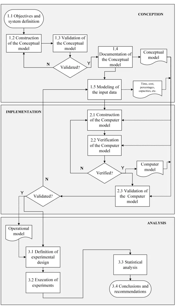
Authors such as Chwif (1999) and Montevechiet al. (2007) show a sequence of steps for a simulation project, countering the false idea that simulation consists only in the model’s com-puter programming. Figure 1, proposed by Montevechiet al. (2007), presents a method of the steps for a simulation project, highlighting the steps of generating conceptual, computational and operational models.

The positioning of verification and validation activities, before the experimental phase, can be observed in Figure 1. These activities might ensure that the model actuallyrepresents the real system, within the limits that were set for the model. Although Figure 1 shows the activities of verification and validation at specific points, these actions occur throughout the simulation project. The actions taken by those responsible for building the model are directly related to V&V activities, from designing the conceptual model to planning scenarios to be tested. The positioning of these activities in Figure 1 aims to highlight moments of the project in which the verification and validation should be properly discussed and documented.

The flowchart in Figure 1 highlights the presence of three models that characterize their res-pective stages. The conceptual model must be validated to be converted into a computational model. The computational model validated is claimed to be operational (operational model or experimental model), and is able to carry out the experiments. The procedures chosen for the definition and execution of experiments (e.g. DOE) must have proper mechanisms of validation (residue analysis). Thus, here the computational model validated is not separated into operational or experimental model, since in practice they represent the same model.

(4)

(5)

the entity, of resources and of controls used, etc. The use of conceptual model for these purposes can be found in works such as Lealet al.(2008) and Lealet al.(2009).

The use of the conceptual model can assist in face-to-face validation (shown in Section 3), along with the use of animation of the simulation. However, the validation of the computational model does not only occur with the use of the conceptual model. Statistical techniques should also be applied in order to show that the computational model, within its domain of applicability, behaves with satisfactory accuracy and consistency with the objectives of the study.

According to Chwif & Medina (2007), two important characteristics of validation should always be taken into consideration:

a) there is no way to 100% validate a model or to ensure it is 100% valid; and

b) there is no guarantee that a model is totally free of bugs. Thus, although the model can be checked for a given circumstance, there is no guarantee that, for any circumstances it works as intended.

The issue of validation involves not only the technical aspect. A complete overview of the process of modeling and simulation also involves art and science (Kleijnen, 1995). In respect to the model, authors such as Harrel & Tumay (1997) emphasize that it should be valid in the sense of satisfactorily representing reality and only including elements that influence the problem to be solved.

Balci (2003) made some considerations about the process of model verification and validation. According to the author, the results of verification and validation should not be considered as a binary variable, where the model being simulated is absolutely correct or absolutely incorrect. A simulation model is built in compliance with the objectives of the modeling and simulation projects, and its credibility is judged according to these goals. The author also writes that, the validation of simulation models, as well as verification, is a difficult process that requires creati-vity and insight.

Some validation techniques are more subjective, using the experience of specialists of the mode-led system to validate the simulation model. However, this type of validation hardly ensures the results obtained for simulated experiments. Statistical research on data obtained in the simula-tion and on historical data (real) of the simulated system is necessary, whenever possible, , thus making it an operational model.

Operational validation is understood as validation of the computational model (Fig. 1), defining it as suitable for the carrying out of experiments, within the limits set in the simulation project’s objectives. This differentiation is important, as another validation is carried out in the conceptual model in a previous step to obtain the computational model, as shown in Figure 1.

(6)

and optimizations by using simulation models without providing information about operational validation process (Ahmed & Alkhamis, 2009; Ekren & Ornek, 2008; Ekrenet al., 2010; Meade

et al., 2006; Sandanayakeet al., 2008).

As for authors such as Bekker & Viviers (2008); Longo (2010); Nazzalet al. (2006) and Kous-kouras & Georgiou (2007), they validated operational models by using more subjective techni-ques, as face-to-face validation, Turing test and animation, present in some simulation softwares. Item 3 of this article will discuss some of these techniques.

Another operational validation used is the comparison of simulation and real system results, using the average and standard deviation of the results (Potteret al., 2007).

Finally, there are authors (Abdulmalek & Rajgopal, 2007; Lam & Lau, 2004; Jordanet al., 2009; Mahfouzet al., 2010) who carry out operational validation also through some form of statistical test, such as building confidence intervals.

Given this diversity of validation forms used by the authors in the area, this article aims to develop a practical guide for operational validation in a more objective way. Some of the techniques mentioned above will be presented in the following item.

3 OPERATIONAL VALIDATION TECHNIQUES

According to Bankset al. (2005), validation can be performed through a series of tests, some of them subjective and some others objective. According to these authors, subjective tests often involve people who know some or many aspects of the system, making judgments about the mo-del and its outputs. The so-called objective tests always require data about the system’s behavior as well as corresponding data produced by the model, in order to compare some aspect of the system with the same aspect of the model, through one or more statistical tests.

Although this article focuses the statistical validation of the computational model, it is not inten-ded to devalue other validation techniques. Kleijnen (1995) states in his article that analysts and users of simulation model must be convinced of its validity, not only by statistical techniques, but also by the application of other procedures, such as the use of animation to assist face-to-face validation or the use of Turing tests. As such, according to the same author, simulation will continue to be both an art and a science.

Some techniques for validation of models are presented by Sargent (2009). The author attributes these techniques to computational model validation. It is noteworthy that some of these techni-ques are more subjective and others more objective, according to the statement of Banks et al.

(2005), presented at the beginning of this item.

• Animation: the operational performance of the model is graphically shown as the model

evolves over time;

• Validation by events: the events of the simulation model are compared to those of the real

(7)

• Face-to-face validation: individuals who know the system are asked if the model behavior

is reasonable;

• Internal validity: different replicas of a stochastic model are made to determine the amount

of variability of the model. A large variability can lead to questioning of the results;

• _{Operational Graphics: values of several performance measures, such as the queue size and}

the percentage of busy servers, are shown graphically as the model evolves over time;

• Sensitivity analysis: this technique consists of changing values of inputs and internal

pa-rameters of a model to determine the effect on the behavior and output of the model. The same relationships should occur between model and real system;

• _{Predictive validation: the model is used to predict the behavior of the system, then these}

predictions are compared with the behavior of the system;

• Turing test: consists in presenting the data generated by the real and the simulated model,

randomly, for individuals who know the operations of the system being modeled. These in-dividuals are then asked whether they can distinguish the outputs of both simulated model and actual system;

• _{Validation by historical data: if there are historical data (data collected in the system), part}

of the data is used to build the model and the rest of the data is used to determine whether the model behaves like the real system.

In the literature concerning statistical procedures, authors such as Chung (2004) highlight some tests, such as the F test. In his opinion, only one version of the test is required for simulation practitioners. This version is represented by equation (1):

F = S

2

M

S2

m

(1)

In Equation 1, where:

• _S2

M is the variance of the data set of highest variance;

• _S_m2 _{is the variance of the data set of lowest variance.}

In this case, we have the following Null Hypothesis: the variances of both sets of data (real system and model) are similar. The Alternative Hypothesis points to no similarity between the sets of variance. It is necessary to select the significance levelαand to determine the critical value forF. Calculating the value of F by equation (1), the Null Hypothesis is rejected if this value exceeds the critical value (taken from a table ofF-Snedecor distribution).

(8)

averages of both sets are equal. The Alternative Hypothesis points to the non-equality between the averages of the two sets.

The Smith-Satterthwaite method is used for cases in which data of the system and the model are normal, but with different variance. This test considers the differences in variances by adjusting the degrees of freedom for a criticaltvalue (taken from a table oft-Student distribution).

The application of this model begins by calculating the number of degrees of freedom, using equation (2), whered f represents the number of degrees of freedom,s₁2the variance of the first set,s₂2the variance of the second set,n1number of elements of the first set andn2 number of elements of the second set.

d f =

s₁2 n1

+s

2 2

n2

!2

s2 1

n1

2

(n1−1)

+

s2 2

n2

2

(n2−1)

(2)

Once the number of degrees of freedom is determined, a t-test is executed. It is important to highlight that, until this point, the data sets evaluated were considered parametric. To Montgo-mery & Runger (2003), traditionally, parametric methods are procedures based on a particular parametric family of distributions, which in this case is normal.

According to Montgomery & Runger (2003), when the distribution under study is not characte-rized as normal, non-parametric methods become very useful. Thus, in situations in which both sets of data are not considered normal, or either one of them, a non-parametric test is used, such as a Mann-WhitneyU test. No assumption about the population distribution in nonparametric methods is made, except that it is continuous.

In the Mann-WhitneyUtest, given two independent samples, the null hypothesis is tested to see whether the median of two samples are equal. It is said, then, that this test is the nonparametric alternative to thettest for difference of means.

The choice of parametric or nonparametric methods is preceded by the assumption that the dis-tribution is continuous. However, some response variables may be characterized as discrete. In this case, authors like Bisgaard & Fuller (1994); Lewiset al. (2000) and Montgomery (2001) recommend performing a transformation to stabilize the variance before applying statistical te-chniques for the operational validation. According to these researchers, when scores are used as an experimental response, the assumption made of constant variance is violated. These authors indicate, in their work, transformation functions appropriate for each case.

(9)

a) non-stationary system – in some systems, you may need to collect the input data and validate them at different times. If the distributions of input data differentiate over time, the process is considered non-stationary. Systems can be non-stationary due to seasonal or cyclical changes. Two approaches can be used: one is the incorporation of non-stationary components of the system in the model, as the inclusion of the distributions of input data that vary over time; and the other is data collection and validation at the same point of time. The second approach provides a model valid only for the conditions under which the input data were obtained;

b) poor input data – data in insufficient quantity and/or precision. In the case of using histo-rical data, the situation in reality may have changed, and

c) invalid assumptions – over-simplified or even poorly modeled.

4 DEVELOPMENT AND IMPLEMENTATION OF THE PROPOSED GUIDE

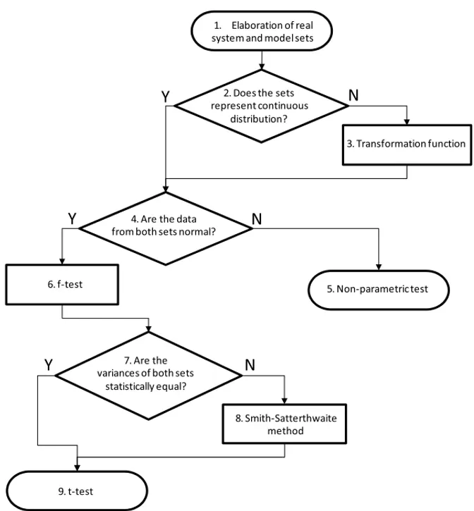
Through analysis of literature, especially in the areas of applied statistics and discrete event simulation, a guide was elaborated in the form of a diagram, with the purpose of guiding those interested in simulation projects in the stage of operational validation of the model. This guide is illustrated in Figure 2.

The first step of this guide suggests participants of the simulation project to organize the infor-mation obtained from the simulation model and the real system into two sets. This inforinfor-mation is from an output variable, such as: total pieces produced, lead time, number of people in line, waiting time, etc. The choice of variable (or variables) is directly related to the objectives of the project.

Based on this step, the guide suggests a sequence of statistical tests, with some decisions to make concerning the nature of the distribution and normality or of the non-distribution and equality (or inequality) of variances. These tests and decisions are scattered throughout the literature, as presented in Section 3. The objective of this guide is to organize these tests and to assist researchers, students and professionals in the stage of operational validation of the simulation model.

To illustrate the applicability of the guide, two objects of study are presented. The first object of study is intended to illustrate the operational validation in which results of the simulation model and the real system have similar variances.

(10)

Figure 2– Guide prepared for operational validation of simulation models (Y = yes, N = no).

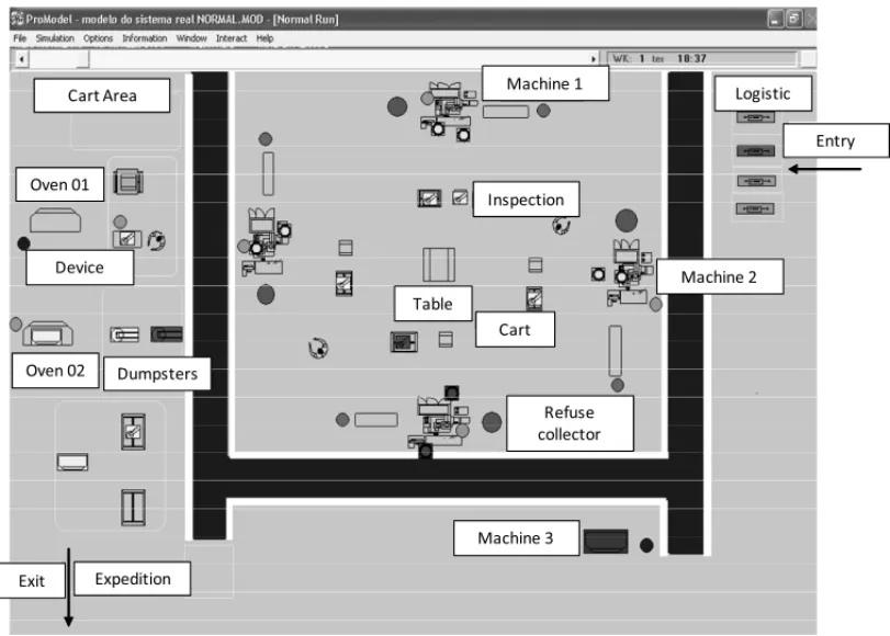
Initially, a conceptual model was built to represent the flow of cell production process and to help in building the computational model. After the validation of the conceptual model by experts, it was converted into a computational model using Promodelrsimulator. Figure 3 shows the screen of the computational model generated after building 16 successive versions of the model. Building in versions allows more efficient model verification (Chwif & Medina, 2007; Banks, 1998; Kleijnen, 1995).

(11)

ENTRADA

SAÍDA

Figure 3– Screen from Promodelrsimulation software, showing the graphic elements of the model for object of study 1.

Having defined the sets, the first decision-making represented in this guide is analyzed. This decision-making is step number two of the guide (Fig. 2).

The result obtained in the simulation model (parts produced per day) could be interpreted as a count in an interval of time, characterizing a typical case of Poisson distribution (Montgomery & Runger, 2003). Therefore, this distribution would be characterized as discrete.

However, when performing a test of adherence to a normal distribution, both sets (real and si-mulated) were accepted in this distribution. As shown in Figure 4, the data can be represented by a normal distribution, since the p-value was higher than 0.05 (significance level). This can be explained as follows: replicas were made and their average was used for validation. This fact is also confirmed by the central limit theorem, which states that whenever a random experiment is replicated, a random variable equal to the average result of the replicas tend to have a normal distribution, as the number of replicas becomes large (Montgomery & Runger, 2003). Thus, step number two of the guide points to continuous distribution.

(12)

P R A C T IC A L G U ID E F O R O P E R A T IO N A L V A L ID A T IO N O F D IS C R E T E S IMU L A T IO N MO D E L S 1600 00 1400 00 1200 00 1000 00 8000 0 6000 0 4000 0 Median Mean

1st Quartile 61109

Median 88560

3rd Quartile 109600

Maximum 153468 69461 104219 67744 104023 24093 50478 A-Squared 0,29 P-Value 0,580 Mean 86840 StDev 32615 Variance 1063733733 Skewness 0,072777 Kurtosis 0,135290 N 16 Minimum 32199

Anderson-Darling Normality Test

95% Confidence Interval for Mean

95% Confidence Interval for Median

95% Confidence Interval for StDev 60000 80000 100000 120000 140000

Median Mean

1st Quartile 81250

Median 105300

3rd Quartile 124475

Maximum 139100 88579 116983 90582 123808 19688 41250 A-Squared 0,42 P-Value 0,281 Mean 102781 StDev 26653 Variance 710356292 Skewness -0,674019 Kurtosis -0,442699 N 16 Minimum 48100

95% Confidence Interval for StDev

(13)

Table 1– Elaboration of data sets for the first step of the guide.

Day Average of parts produced per day Parts produced per day in the 10 replicas of simulation model in the real system

1 48100 32400

2 94900 87308

3 120900 93422

4 104000 89162

5 72800 32199

6 123500 83019

7 94900 112647

8 139100 88941

9 76700 112319

10 119600 88179

11 131300 55743

12 61100 70815

13 124800 130502

14 100100 57874

15 126100 101442

16 106600 153468

It is not the scope of this paper to discuss the transformation functions. As such, the following reading is suggested: Bisgaard & Fuller (1994); Lewiset al.(2000) and Montgomery (2001).

After verifying that simulated and real sets represent continuous distributions, or after the trans-formation function (steps 2 and 3 of the guide), step number 4 is performed. In this step, there is a test of adherence for normal distribution.

In this first object of study, data from two sets could be represented by a normal distribution, according to the normality test performed (Anderson-Darling), shown in Figure 4. If one or both sets of data do not characterize a normal distribution, we use a nonparametric test (step number five of the guide) as presented in Section 3 of this article. One of these tests is the Mann-Whitney

Utest. In this, the objective is to test the null hypothesis, which is that the two sets have equal medians. The operational validation of the model, in the case of sets of non-parametric data, ends in step 5. Further details can be found in Montgomery & Runger (2003).

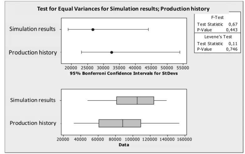
As in the first object of study, the sets assumed normal distributions and anF-test was performed, as indicated in step number 6 of the guide. The purpose of the F-test is to test the hypothesis that both data sets (real and simulated) have equal variances. Figure 5 shows the result of F-test on the first object of study.

(14)

Hist órico de produção Result ados da simulação

55000 50000 45000 40000 35000 30000 25000 20000

Hist órico de produção Result ados da simulação

160000 140000 120000 100000 80000 60000 40000 20000

T est St at ist ic 0,67 P-V alue 0,443

T est St at ist ic 0,11 P-V alue 0,746

F-T est

Levene's T est

Figure 5–F-test performed on the first object of study: equal variances,p-value 0.443.

After the t-test, it is possible to affirm that the computational model of real system is statisti-cally validated, since p-value is 0.141. It is said then that the computer model is able to receive experimentations in this output variable analyzed. After this, the operational model of the manu-facturing cell under study is obtained.

To illustrate the use of step 8, we present the second object of study. In the second application of the operational validation guide, it is intended to illustrate the operational validation in which results of the simulation model and the real system do not have similar variances.

The second study object is a cell for assembling optical transponders from Padtec S/A, a Bra-zilian technological company. Transponders mounted by this cell represent about 40% of the company’s sales revenue, while the second product in revenue represents 20%. This cell has specific optical equipment for the testing of the transponders, work benches and computers. Two employees perform activities of the production process, allocated on a single production shift.

Similar to the first object of study, the conceptual model was built and validated by the engine-ers responsible for production. Then, this conceptual model was implemented in the simulator Promodelr. Twelve models were built, in increasing order of complexity, until a model was achieved to be submitted to the operational validation process. Figure 6 shows the screen of the computer model, built with software Promodelr.

(15)

Figure 6– Screen of Promodelrsimulation software, showing the graphic elements of the model for the object of study 2.

was used to indicate possible programming errors. Counters were also placed along the model for spot checks.

After verification, face-to-face validation was performed. By means of graphic animations, ex-perts were able to evaluate the system’s behavior. In this more subjective test, the computational model was validated.

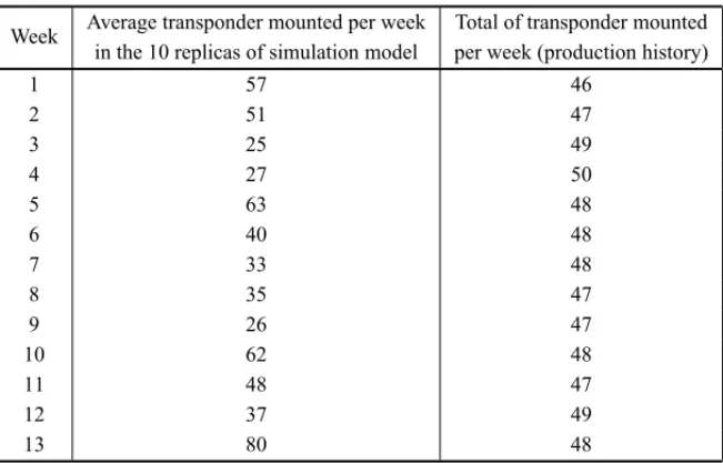
After this face-to-face validation, the guide of operational validation was applied. To this end, the model was run for thirteen weeks, with ten replicas each. The weekly amount of parts pro-duced was measured by the average of these values (considering the ten replicas). At the same time, values for total transponders mounted per week in the real system were obtained from the company’s ERP system for the same period. Table 2 shows these results.

After completing the first step of the guide, there was an adherence test for the normal distribu-tion, and it was found that these data can be adjusted this way. As shown in Figure 7, a finding of continuous and normal distribution leads the analysis to step 6 of the guide.

(16)

P R A C T IC A L G U ID E F O R O P E R A T IO N A L V A L ID A T IO N O F D IS C R E T E S IMU L A T IO N MO D E L S 50 49 48 47 46 Median Mean 48,5 48,0 47,5

1st Quartile 47,200

Median 48,100

3rd Quartile 48,700

Maximum 49,900 47,346 48,546 47,200 48,589 0,712 1,639 A-Squared 0,21 P-Value 0,835 Mean 47,946 StDev 0,993 Variance 0,986 Skewness 0,272628 Kurtosis 0,030679 N 13 Minimum 46,200

95% Confidence Interval for StDev 30 40 50 60 70 80

Median Mean

60 45

30

1st Quartile 30,000

Median 40,000

3rd Quartile 59,500

Maximum 80,000 34,684 55,162 31,108 58,577 12,150 27,969 A-Squared 0,33 P-Value 0,472 Mean 44,923 StDev 16,943 Variance 287,077 Skewness 0,654602 Kurtosis -0,327246 N 13 Minimum 25,000

95% Confidence Interval for StDev

(17)

Table 2– Elaboration of data sets for the first step of the guide.

Week Average transponder mounted per week Total of transponder mounted in the 10 replicas of simulation model per week (production history)

1 57 46

2 51 47

3 25 49

4 27 50

5 63 48

6 40 48

7 33 48

8 35 47

9 26 47

10 62 48

11 48 47

12 37 49

13 80 48

does not invalidate the model. It allows for decision making in step 7 of the guide, leading the validation to step 8.

Step 8 can be accomplished either in algebraic form, as indicated in this article, or via software. Minitabr, for example, presents the possibility for the user to select the option of non-equality of variances beforet-test.

It is noteworthy that this result was discussed with the process engineers and the great variability observed in the production history is consistent with the production strategy adopted by the company in question, i.e., there are weeks with a large volume of transponders mounted and in other weeks, however, low volume of transponders mounted. In a given week, for example, there may have been a late arrival of imported materials, which may have come earlier next week, thus presenting a large production. As the simulation model is a simplification of reality, it cannot incorporate this great variability.

Immediately after step 8 (applied to the case of non-equal variances), one can then perform a

t test for two independent samples, which tests the equality of averages for simulated and real data, taking into account the non-equality of variances. As the test showed p-value equal to 0.533 (greater than 0.05), hypothesis of the simulation model validity is accepted.

(18)

This experiment consisted in eliminating an activity of the manufacturing cell’s production flow (just like it was done in a scenario of the simulation model). This scenario was chosen because the simulation model showed a 40% increase in monthly production of the cell by eliminating this activity. This confirmation experiment revealed a real monthly production very close to that predicted by the simulation model. Experiments of this nature increase the credibility of the model for those who will actually make the decisions with the help of the model.

5 CONCLUSIONS

This paper presented two research questions. The first asked what were the forms found for operational validation of discrete simulation models in the literature. Through a summarized literature review in items 2 and 3 of this article, it was possible to verify that, in the scientific literature (specifically in the area of modeling and simulation), there are articles that use more subjective forms of operational validation, while others use more objective forms (statistical techniques). Moreover, among these articles, some (as shown) had no details of the operational validation. This survey underlines the need of a practical guide for operational validation.

The second question presented in this paper suggests the creation of a practical guide for ope-rational validation. This guide was created and presented in item 4 of this article. This item also presented the application of the guide in two objects of study. Each step of the guide was presented and discussed within the situations encountered on the objects of study.

Although the techniques used in the guide already exist in the literature, they are scattered th-roughout publications in the field of statistics. The sequencing of these techniques, according to decisions to be made by those responsible for the modeling, composes this practical guide. The expected effect of the creation of this guide is not restricted only to aid the design of simulation in companies, but also in scholarly works. Several academic studies have been oriented by the authors of this paper using the guide. It is possible to conclude that of these orientations using the guide, there is a great increase in interest, on the part of students (undergraduate and graduate), in ensuring operational validation of their models in a documented way in their works.

The proposed use of the operational validation guide does not suggest the elimination of subjec-tive techniques for validating the computational model. As presented in this article, techniques such as face-to-face validation and Turing test are used in articles published in journals and con-gresses. The combination of these subjective techniques with the use of the guide here presented may improve this difficult process of operational validation, considered by some authors (cited in this article) as a mixture of art and science.

ACKNOWLEDGEMENTS

(19)

REFERENCES

[1] ABDULMALEKFA & RAJGOPALJ. 2007. Analyzing the benefits of lean manufacturing and value stream mapping via simulation: A process sector case study.International Journal of Production Economics,107: 223–236.

[2] AHMED MA & ALKHAMIS TM. 2009. Simulation optimization for an emergency department healthcare unit in Kuwait.European Journal of Operational Research,198: 936–942.

[3] BALCIO. 1997. Verification, validation and accreditation of simulation models. In: Proceedings of the 1997 Winter Simulation Conference, Atlanta, GA, USA.

[4] BALCIO. 2003. Verification, validation, and certification of modeling and simulation applications. In: Proceedings of the 2003 Winter Simulation Conference, New Orleans, Louisiana, USA.

[5] BANKS J. 1998. Handbook of simulation: Principles, Methodology, Advances, Applications, and Practice. Ed. John Wiley & Sons, Inc., 864p.

[6] BANKSJ, CARSONJS, NELSONBL & NICOLDM. 2005. Discrete-event Simulation. 4 ed. Upper Saddle River, NJ: Prentice-Hall.

[7] BEKKER J & VIVIERSL. 2008. Using computer simulation to determine operations policies for a mechanised car park.Simulation Modelling Practice and Theory,16: 613–625.

[8] BISGAARDS & FULLERH. 1994. Analysis of Factorial Experiments with defects or defectives as the response. Report n. 119, Center for Quality and Productivity Improvement University of Wisconsin.

[9] BOXGEP, LUCENO˜ A & PANIAGUA-QUINONES˜ MC. 2009. Statistical control by monitoring and adjustment. 2 ed. Ney Jersey: John Wiley & Sons.

[10] CHUNGCA. 2004. Simulation Modeling Handbook: a practical approach. Washington D.C: CRC press, 608p.

[11] CHWIF L. 1999. Redução de modelos de simulação de eventos discretos na sua concepção: uma abordagem causal. 1999. 151 f. Tese (Doutorado em Engenharia Mecânica) – Escola Politécnica, Universidade de São Paulo, São Paulo.

[12] CHWIFL & MEDINAAC. 2007. Modelagem e Simulação de Eventos Discretos: Teoria e Aplicaç ões. São Paulo: Ed. dos Autores, 254p.

[13] EKREN BY & ORNEK AM. 2008. A simulation based experimental design to analyze factors affecting production flow time.Simulation Modelling Practice and Theory,16: 278–293.

[14] EKREN BY, HERAGU SS, KRISHNMURTHTY A & MALMBORG CJ. 2010. Simulation based experimental design to identify factors affecting performance of AVS/RS.Computers & Industrial Engineering,58: 175–185.

[15] GARZA-REYESJA, ELDRIDGES, BARBERKD & SORIANO-MEIERH. 2010. Overall equipment effectiveness (OEE) and process capability (PC) measures: a relationship analysis. International Journal of Quality & Reliability Management,27(1): 48–62.

[16] HARREL C, GHOSH BK & BOWDEN RO. 2004. Simulation Using Promodel. 2 ed. New York: McGraw-Hill.

(20)

[18] JORDAN JD, MELOUK SH & FAAS PD. 2009. Analyzing production modifications of a c-130 engine repair facility using simulation. In: Proceedings of the Winter Simulation Conference, Austin, Texas, USA.

[19] KLEIJNENJPC. 1995. Theory and Methodology: Verification and validation of simulation models.

European Journal of Operational Research,82: 145–162.

[20] KOUSKOURAS KG & GEORGIOU AC. 2007. A discrete event simulation model in the case of managing a software project.European Journal of Operational Research,181: 374–389.

[21] KUMAR S & SRIDHARAN R. 2007. Simulation modeling and analysis of tool sharing and part scheduling decisions in single-stage multimachine flexible manufacturing systems. Robotics and Computer-Integrated Manufacturing,23: 361–370.

[22] LAMK & LAURSM. 2004. A simulation approach to restructuring call centers.Business Process Management Journal,10(4): 481–494.

[23] LAWAM. 2006. How to build valid and credible simulation models. In: Proceedings of the 2006 Winter Simulation Conference, Monterey, CA, USA.

[24] LEAL F. 2003. Um diagnóstico do processo de atendimento a clientes em uma agência bancária através de mapeamento do processo e simulação computacional. 224 f. Dissertação (Mestrado em Engenharia de Produção) – Universidade Federal de Itajubá, Itajubá, MG.

[25] LEALF, ALMEIDADADE& MONTEVECHIJAB. 2008. Uma Proposta de Técnica de Modelagem Conceitual para a Simulação através de elementos do IDEF. In: Anais do XL Simp ósio Brasileiro de Pesquisa Operacional, João Pessoa, PB.

[26] LEALF, OLIVEIRAMLMDE, ALMEIDADADE& MONTEVECHIJAB. 2009. Desenvolvimento e aplicação de uma técnica de modelagem conceitual de processos em projetos de simulação: o IDEF-SIM. In: Anais do XXIX Encontro Nacional de Engenharia de Produção, Salvador, BA.

[27] LEWISSL, MONTGOMERYDC & MYERS RH. 2000. The analysis of designed experiments with non-normal responses.Quality Engineering,12(2): 225–243.

[28] LONGOF. 2010. Design and integration of the containers inspection activities in the container termi-nal operations.International Journal of Production Economics, article in press.

[29] MAHFOUZA, HASSANSA & ARISHA A. 2010. Practical simulation application: Evaluation of process control parameters in Twisted-Pair Cables manufacturing system. Simulation Modelling Practice and Theory, article in press.

[30] MEADEDJ, KUMAR S & HOUSHYAR A. 2006. Financial analysis of a theoretical lean manu-facturing implementation using hybrid simulation modeling. Journal of Manufacturing Systems, 2(25): 137–152.

[31] MONTEVECHI JAB, PINHO AF DE, LEAL F & MARINS FAS. 2007. Application of design of experiments on the simulation of a process in an automotive industry. In: Proceedings of the 2007 Winter Simulation Conference, Washington, DC, USA.

[32] MONTGOMERYDC. 2001. Design and analysis of experiments. 5th ed. John Wiley & Sons: New York.

(21)

[34] MOSQUEDA MRP, TOLLNEREW, BOYHAN GE, LIC & MCCLENDON RW. 2009. Simulating onion packinghouse product flow for performance evaluation and education.Biosystems Engineering, 102: 135–142.

[35] NAZZAL D, MOLLAGHASEMI M & ANDERSON D. 2006. A simulation-based evaluation of the cost of cycle time reduction in Agere Systems wafer fabrication facility – a case study.International Journal of Production Economics,100: 300–313.

[36] POTTERA, YANGB & LALWANIC. 2007. A simulation study of despatch bay performance in the steel processing industry.European Journal of Operational Research,179: 567–578.

[37] RAJAR & RAOKS. 2007. Performance evaluation through simulation modeling in a cotton spinning system.Simulation Modelling Practice and Theory,15: 1163–1172.

[38] ROBINSON S. 2007. A statistical process control approach to selecting a warm-up period for a discrete-event simulation.European Journal of Operational Research,176: 332–346.

[39] SANDANAYAKEYG, ODUOZACF & PROVERBSDG. 2008. A systematic modelling and simulation approach for JIT performance optimisation.Robotics and Computer-Integrated Manufacturing,24: 735–743.

[40] SARGENTRG. 2009. Verification and validation of simulation models. In: Proceedings of the Winter Simulation Conference, Austin, Texas, USA.

[41] VAN VOLSEM S, DULLAERTW & VANLANDEGHEMH. 2007. An Evolutionary Algorithm and