www.ann-geophys.net/25/255/2007/ © European Geosciences Union 2007
Annales
Geophysicae
The mechanical advantage of the magnetosphere: solar-wind-related
forces in the magnetosphere-ionosphere-Earth system
V. M. Vasyli ¯unas
Max-Planck-Institut f¨ur Sonnensystemforschung, 37191 Katlenburg-Lindau, Germany Received: 20 November 2006 – Accepted: 22 January 2007 – Published: 1 February 2007
Abstract. Magnetosphere-ionosphere interactions involve electric currents that circulate between the two regions; the associated Lorentz forces, existing in both regions as matched opposite pairs, are generally viewed as the primary mechanism by which linear momentum, derived ultimately from solar wind flow, is transferred from the magnetosphere to the ionosphere, where it is further transferred by colli-sions to the neutral atmosphere. For a given total amount of current, however, the total force is proportional to LB
and in general, sinceL2B∼constant by flux conservation, is much larger in the ionosphere than in the magnetosphere (L = effective length, B = magnetic field). The magneto-sphere may be described as possesing a mechanical advan-tage: the Lorentz force in it is coupled with a Lorentz force in the ionosphere that has been amplified by a factor given approximately by the square root of magnetic field magni-tude ratio (∼20 to 40 on field lines connected to the outer magnetosphere). The linear momentum transferred to the ionosphere (and thence to the atmosphere) as the result of magnetic stresses applied by the magnetosphere can thus be much larger than the momentum supplied by the solar wind through tangential stress. The added linear momen-tum comes from within the Earth, extracted by the Lorentz force on currents that arise as a consequence of magnetic per-turbation fields from the ionosphere (specifically, the shield-ing currents within the Earth that keep out the time-varyshield-ing external fields). This implies at once that Fukushima’s the-orem on the vanishing of ground-level magnetic perturba-tions cannot be fully applicable, a conclusion confirmed by re-examining the assumptions from which the theorem is derived. To balance the inferred Lorentz force within the Earth’s interior, there must exist an antisunward mechanical stress there, only a small part of which is the acceleration of the entire Earth system by the net force exerted on it by the
Correspondence to:V. M. Vasyli¯unas ([email protected])
solar wind. The solar-wind interaction can thus give rise to internal forces, significantly larger than the force exerted by the solar wind itself, between the ionosphere and the neutral atmosphere as well as within the current-carrying regions of the Earth’s interior.
Keywords. Ionosphere (Ionosphere-atmosphere inter-actions) – Magnetospheric physics (Magnetosphere-ionosphere interactions; Solar wind-magnetosphere interac-tions)
1 Introduction
More recently, attention has increasingly been directed to-ward the possible contribution of drag forces on the high-latitude ionosphere, associated with the tangential stress of the solar wind and mediated by Birkeland (magnetic-field-aligned) currents between the ionosphere and the outer magnetosphere, in particular the so-called region 1 currents (Iijima and Potemra, 1976). Siscoe et al. (2002) propose that, in the limit of very strong solar wind interaction (transpolar potential saturation regime), stresses associated with region 1 currents assume the dominant role in transmitting forces exerted by and on the solar wind.
In all these discussions it appears mostly to have been taken for granted that the linear momentum supplied by the solar wind is simply transferred to the other regions and that any force exerted on the ionosphere or on the Earth is equal to the force applied by the solar wind. The purpose of this paper is to point out that this is not the case: as a conse-quence of very simple considerations of magnetic field ge-ometry, any given current system flowing between the mag-netosphere and the ionosphere implies a much larger Lorentz force in the ionosphere than it does in the magnetosphere. This conclusion has been reached independently by Siscoe and Siebert (2006) for the special case of forces associated with region 1 currents, in the context of a general discussion of solar wind forces on the magnetosphere and their rela-tion to observed thermospheric effects during large magnetic storms.
In effect, as far as Lorentz forces are concerned, the mag-netosphere may be said to act on the ionosphere as a simple machine (e.g. lever or pulley) with a very considerable me-chanical advantage. A force applied by the solar wind may then appear as a much larger force on the ionosphere, rais-ing the question (since linear momentum is conserved) where the excess linear momentum is coming from. I show that it is coming from Lorentz forces exerted on currents within the Earth’s interior that arise as the result of the disturbance fields from the ionosphere; the various arguments commonly made (notably the celebrated theorem of Fukushima, 1969, 1971, 1985b) that these disturbance fields are unimportant below the ionosphere must therefore be of limited applicability.
2 Mechanical and electromagnetic stress balance equa-tions
Conservation of linear momentum in an extended medium is discussed in any textbook of fluid mechanics or plasma physics (see, e.g., Landau and Lifshitz, 1959; Rossi and Olbert, 1970; Siscoe, 1983, the latter a treatment intended specifically for magnetospheric applications). The local (dif-ferential) form of the momentum equation (written in the standard conservation form: partial time derivative of den-sity of conserved quantity plus divergence of flux denden-sity of conserved quantity) is
∂G/∂t+∇·(ρV V +P−T)=0 (1)
where
G=ρV +(E×B/4π c) (2) is the linear momentum per unit volume, the first term rep-resenting the momentum of bulk flow of the medium and the second the momentum of the electromagnetic field (I use Gaussian units throughout);ρ,V, andPare, respectively, the mass density, bulk flow velocity, and pressure tensor of the medium;Tis the sum of the Maxwell stress tensorTM (the divergence of which is equal to the Lorentz force per unit volume) plus the stress tensors representing any other forces. The global form of the momentum equation, obtained by in-tegrating Eq. (1) over a given volume, states that the total lin-ear momentum contained within the volume changes at a rate that is given by a surface integral over the boundary of the volume; the three terms in the surface integral, correspond-ing to the three terms within the divergence in Eq. (1), repre-sent the net rate of momentum transfer across the boundary by bulk flow (first term), by thermal motion of particles (sec-ond term: pressure tensor), and by the action of forces on the medium (third term: stress tensors of the various forces). That the total force acting on the medium within the vol-ume can be expressed as the surface integral of the appropri-ate stress tensor is an essential condition for conserving total linear momentum. For an isolated system, with negligible surface terms, the total linear momentum remains constant.
Under the usual assumptions of charge quasi-neutrality of the plasma, nonrelativistic bulk flows, and Alfv´en speed
VA2≪c2, the electromagnetic contribution to the linear mo-mentum density (second term on the right-hand side of Eq. (2) and the electric-field terms in the Maxwell stress ten-sor can be neglected. The Lorentz force then reduces to just the magnetic force, given by the divergence of the Maxwell stress tensor
J×B/c=∇·TM =∇· h
BB/4π−IB2/8πi (3) (Iis the unit dyad,Iij=δij); to derive relation (3), Amp`ere’s law
J=(c/4π )∇ ×B (4)
needs to be invoked.
For the purposes of this paper, three aspects of the above general formulation, embodied in Eqs. (4), (3), and (1), are important:
1) Equation (4) implies the current continuity condition ∇·J=0, which is the basis for the results discussed in Sect. 3. 2) Equation (1) in its integral form, applied to a sequence of nested boundary surfaces from the magnetopause inward to the center of the Earth, forms the basis for the discussion in Sect. 5 of linear momentum transfer from the solar wind.
to Fukushima’s theorem discussed in Sect. 6. Foranychosen volume, the total Lorentz force exerted on currents within the volume can be calculated in this way, with no constraints from current closure; even if the current does not close within the volume, the total Lorentz force is a well defined physical quantity – in contrast to the magnetic field of an unclosed cur-rent segment, which in general has only a mathematical sig-nificance (Vasyli¯unas, 1999). This force is given, however, by the surface integral of the Maxwell stress tensor, and one may view the surface in two ways: either as the outer bound-ary of the chosen volume, or as the inner boundbound-ary of the rest of space, the difference being only in the sign of the normal vector. Hence the total Lorentz force on currents (closed or unclosed)withinany volume is precisely equal and opposite to the total Lorentz force on currents outsidethat volume; this applies to each Cartesian vector component, taken sep-arately. A corollary is that magnetic fields due entirely to currents confined within a volume exert no net force on the volume.
3 Relation between Lorentz forces in the magneto-sphere and the ionomagneto-sphere
The interaction between the magnetosphere and the iono-sphere proceeds to a large extent by means of electric currents that flow in both regions, coupled by Birkeland (magnetic-field-aligned) currents between the two; much of the classical theory of magnetosphere-ionosphere coupling consists simply of the self-consistency conditions on these currents and on the associated plasma flows and stresses. As a prototypical example, Fig. 1 shows a sketch of the complete system of region 1 currents. The segmentI−I′ flows from dawn to dusk in the polar ionosphere. The segmentM′−M flows from dusk to dawn somewhere in the outer magneto-sphere; the precise location has not been conclusively iden-tified but is generally assumed to be near the magnetopause, its boundary layers, or the adjacent magnetosheath. The seg-mentsM−I andI′−M′ are the region 1 currents proper: Birkeland currents flowing into the ionosphere on the dawn side and out of the ionosphere on the dusk side.
Current continuity imposes a relation between the currents in the different segments. With the segments idealized, for simplicity, as line currents in Fig. 1 (in reality, of course, they have appreciable width in the transverse directions), the relation is simply that the total currentI is the same every-where. The total Lorentz force exerted on the plasma in each segment can now be computed. The segmentsM−I andI′−M′are (very nearly) aligned with the ambient mag-netic field and hence have negligible Lorentz force. At the ionospheric segmentI−I′, the ambient magnetic fieldBi is downward, and the Lorentz forceFiis directed antisunward. At the magnetospheric segmentM−M′, the vertical com-ponent of the ambient magnetic fieldBmis (for the assumed location) likewise downward but, with the current reversed,
✚✙ ✛✘
✛
✲
❄ ✻
✻
I
I′
M
M′
(dawn)
(dusk)
Fig. 1. Schematic diagram of region 1 currents in Northern Hemi-sphere, viewed from above the north pole (Sun to the left).
the Lorentz forceFmin the plane is directed sunward. The magnitude of the forces is
Fi ≈(I /c) BiLi Fm≈(I /c) BmLm (5) whereLi,Lmare the effective lengths of the respective seg-ments; the currentI is the same in both. From conservation of magnetic flux
BiLihi ≈BmLmhm (6)
wherehi,hmare the effective widths of the segments in the direction transverse to the current. From Eqs. (5) and (6), the ratio of the Lorentz force in the ionosphere to that in the magnetosphere is
Fi/Fm≈hm/ hi ≈[(Bi/Bm) (Li/ hi) (hm/Lm)]1/2
∼pBi/Bm (7)
where the last approximation follows from the reasonable assumption that the ratio of width to length does not differ greatly between the two regions.
✁✁❆❆
✻
❄
ionosphere
magnetosphere
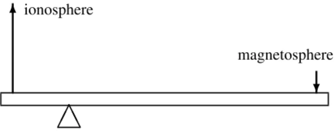
Fig. 2. Relation between forces in ionosphere and magnetosphere for system of region 1 currents (Fig. 1), illustrated by analogy to a simple lever system with mechanical advantage (antisunward is up).
of magnetic field strength – typically a factor∼20 to 40. Sis-coe and Siebert (2006) reached the same conclusion by car-rying out a global MHD simulation of the magnetosphere subject to a strong tangential drag: finding directly that the momentum transfer to the Earth was much larger than that across the magnetopause, they interpreted the difference by a geometrical argument identical to that given here in deriv-ing Eq. (7).
The geometrical argument is in fact quite general and is not restricted to the region 1 current system or direct solar-wind interaction. (For example, Fig. 1 with the sense of all the currents reversed can be viewed as a sketch of the region 2 currents (Iijima and Potemra, 1976), the only other differ-ence being that the closure currentM−M′ in this case is generally thought to be located in the plasma sheet where the ambient magnetic field is upward, hence the Lorentz force on both the magnetospheric and the ionospheric segments is now sunward.) For any system involving currents that cir-culate between the magnetosphere and the ionosphere, the Lorentz force exerted by the ionospheric portion is propor-tional to that exerted by the magnetospheric portion but is also amplified relative to it by a factor, given in Eq. (7), which depends only on the geometrical configuration of the current and of the magnetic field. The situation is analogous to that of a mechanical force amplified by a simple machine, as il-lustrated in Fig. 2 which represents the Lorentz forces of the configuration in Fig. 1 as forces acting on a lever. The ampli-fication factor is often referred to as the mechanical advan-tage of the machine.
A further property shared by simple machines and by Lorentz forces in the magnetosphere-ionosphere system is that whereas force is amplified, energy is not. A suitable lever may greatly reduce the force one must apply to raise a given weight, but it does not change at all the amount of work one must do in raising it. Similarly, the rate of electromag-netic energy conversion is given by current times potential difference; the total current is the same in both regions, and as long as the potential difference is the same (analogous to the requirement in the mechanical case that the lever is not being deformed), the rate of energy conversion in the iono-sphere is equal in magnitude (and opposite in sign) to that in the magnetosphere.
4 Implications of amplified Lorentz force
Given the result (Sect. 2) that the total Lorentz force within a volume must be matched by an equal and opposite Lorentz force somewhere outside the volume, where is this recipro-cal force in the case of the Lorentz force on the ionospheric segment of the magnetosphere-ionosphere current system? It cannot be the magnetospheric segment, the Lorentz force on which is smaller by the amplification factor (Sect. 3) and thus cannot be equal (not to mention the possibility that it may even not be opposite, one counterexample being the re-gion 2 current system). A related question is: given the result (Sect. 3) that the linear momentum being imparted to the neu-tral atmosphere is much larger than that being extracted from the solar wind, where does the additional linear momentum come from?
To the two questions there is a single answer: wherever the reciprocal Lorentz force is located, it extracts linear momen-tum from the surrounding medium. In terms of the mechani-cal analog in Fig. 2, this location corresponds to the fulcrum (support) of the lever, the force through the fulcrum being what maintains overall balance with both the direct and the amplified applied force. In the present case, the location evi-dently must be inward of the ionosphere and hence within the conducting regions of the Earth’s interior; furthermore, the existence of the Lorentz force there must be connected with electromagnetic effects of currents in the ionosphere (this is the only way the ionosphere can act across the intervening poorly conducting atmosphere to influence the Earth’s inte-rior).
It might be argued that, since the excess Lorentz force is exerted by the Earth’s dipole field acting on currents in the ionosphere, it must therefore be balanced by an equal and opposite Lorentz force exerted by the magnetic perturbation fields from the ionosphere acting on the dynamo currents that produce the Earth’s dipole. However, since the Lorentz force has a direction fixed relative to the Sun-Earth line, the mag-netic perturbation fields from the associated currents nec-essarily vary with local time; in a frame of reference fixed to the rotating Earth, they appear as time-varying perturba-tions at the diurnal period and therefore can penetrate into the conducting interior to a depth of no more than about 0.1 or at most 0.2RE (e.g. Price, 1967; Carovillano and Siscoe, 1973), well outside the presumed dynamo region.
5 Linear momentum transfer from the solar wind
The total force exerted on the magnetosphere-ionosphere-atmosphere-Earth system as the result of interaction with the solar wind can be calculated by integrating the divergence term in Eq. (1) over the volume of the entire system and thus can be expressed as the surface integral of the stress tensor over the outer boundary of the volume. (This surface integral is also, by definition, equal to the rate of linear momentum transfer across the surface.) By separating out the Maxwell stress, the total force can be written as the sum of electro-magnetic and mechanical contributions:
FEM = Z
dS·hBB/4π−IB2/8πi (8)
Fmech= − Z
dS·(ρV V +P) . (9)
Gravity is represented by a term in the total stress tensorT (e.g., Siscoe, 1970, 1983) but may alternatively and more conveniently be taken into account by adding the termρg
to the right-hand side of Eq. (1), wheregis the gravitational acceleration. Conservation of linear momentum gives
Fmech+FEM+Mg=(d/dt ) Z
d3rρV (10)
where
M= Z
d3rρ (11)
is the total mass contained within the volume, andg here is only theexternalgravitational acceleration, due predomi-nantly to the gravity of the Sun (hencegis, to a very good approximation, constant over the volume) – there cannot be any net force or acceleration of the entire Earth system by the gravity of its own internal mass.
As shown in Appendix A, the right-hand side of Eq. (10) can be written as simplyMtimes the acceleration of the cen-ter of massR, plus a small correction term. Equation (10) now becomes
Fmech+FEM−δFm=M
d2R/dt2−g (12) where
δFm=2(dM/dt ) (dR/dt )+ Z
dS·(∂ρV/∂t ) (r−R)
= Z
dS·[(∂ρV/∂t ) (r−R)−2ρV(dM/dt )] (13) is a surface integral involving plasma flow and hence can be treated as a correction term to the mechanical force. Note thatδFmis zero if there is no mass flow across the boundary and also vanishes in a steady state or upon time averaging.
Equation (12) can be applied to any chosen volume, and it is instructive to consider a family of volumes obtained by se-quentially displacing the boundary inward: first, the bound-ary outside the magnetopause, enclosing the entire system;
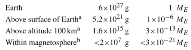
Table 1. Masses in the Earth-ionosphere-magnetosphere system.
Earth 6×1027g 1 ME Above surface of Eartha 5.2×10²¹g 1×10⁻⁶ME Above altitude 100 kma 1.6×10¹⁵g 3×10⁻¹³ME Within magnetosphereb <2×10⁷ g <3×10⁻²¹M
E
aComputed from atmospheric pressure≃weight of overlying mass
per unit area.
bRough upper limit, estimated as mass of solar wind plasma
(pro-ton concentrationnsw=10 cm−3) contained within sphere of radius 10RE.
then the boundary just inside the magnetopause; then just above the ionosphere; then just below the ionosphere; then moving by steps into the interior of the Earth, finally con-verging on the center. For each one of the volumes, the total force on it is determined entirely by quantities on the bound-ary surface only (left-hand side of the equation) and is equal to the net acceleration – inertial minus gravitational – of the total massMcontained within the entire volume (right-hand side). Since the masses in the atmosphere, ionosphere, and magnetosphere are completely negligible in comparison to the mass of the EarthME (Table 1), to an extremely good approximationMis equal toME for all those volumes that include the entire Earth, and the center of massRcoincides with the center of the Earth for all the volumes. The net acceleration (d2R/dt2−g) has for all practical purposes the same value for all the volumes under consideration; Eq. (12) then implies that the total force on any one volume varies only in proportion to the total mass enclosed.
The total force on the magnetosphere alone (the volume between the magnetopause and the ionosphere) can be calcu-lated by subtracting the forces on two volumes, with bound-aries just inside the magnetopause and just above the iono-sphere, respectively. The ratio of the resulting net force on the magnetosphere to the (solar-wind-related) force on the Earth is equal to the ratio of the mass in the magnetosphere to the mass of the Earth and hence is extremely small; this is the quantitative reason for the statement (previously de-rived only qualitatively, Siscoe, 1966; Carovillano and Sis-coe, 1973) that the entire force from the solar wind interac-tion must be transferred to the solid Earth, with negligible net force on the magnetosphere. By the same argument, this holds for other regions (e.g., the ionosphere or even the entire atmosphere), as long as the mass there is much smaller than
ME.
s
✲ ✲ magnetopause
✲ ✲ ionosphere
✛
✲ ✛
✲ shielding currents
✲ ✲ (center of Earth)
(solar wind)
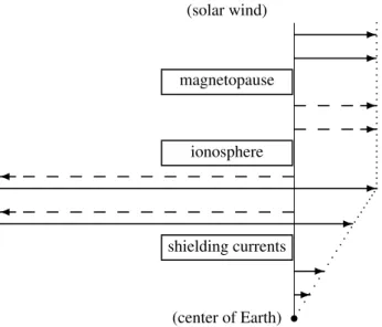
Fig. 3. Total force, calculated from integral of stress tensor over surfaces enclosing varying subvolumes of the Earth-magnetosphere system, separated into mechanical (solid line) and electromagnetic (dashed line) contributions. Arrow to the left (right): force sun-ward (antisunsun-ward). The force at each location acts on the enclosed volume, from the location shown down to the center of Earth.
the total force, without distinction between mechanical and electromagnetic; as discussed above, this force remains con-stant when the boundary surface is displaced inward from the magnetopause, beginning to decrease (in proportion to the enclosed mass) only when the boundary has been taken below the surface of the Earth.
5.1 Linear momentum transfer across the magnetopause For each assumed boundary surface, mechanical and elec-tromagnetic contributions to the integrated force (or, equiv-alently, the integrated rate of linear momentum transfer) can be calculated separately, as illustrated in Fig. 3. The stress tensor on the surface just outside the magnetopause is pre-dominantly mechanical, containing both a pressure contri-bution (magnetosheath plasma pressure, proportional to dy-namic pressure of the solar wind), important primarily on the dayside, and a tangential drag contribution (usually ascribed to magnetic tension inside the magnetopause but, as dis-cussed by Vasyli¯unas, 1987, describable equally well as flow deceleration stress outside the magnetopause), important pri-marily in the magnetotail. The stress tensor on the surface just inside the magnetopause is predominantly electromag-netic, magnetic pressure being most important on the day-side and magnetic tension in the magnetotail (Siscoe, 1966; Siscoe and Siebert, 2006; Siscoe, 2006). The total rate of lin-ear momentum transfer is the same on both sides. Within the interaction region just outside and at the magnetopause, the mechanical antisunward force from the flowing solar wind is
transformed, by the action of Lorentz force balanced every-where by appropriate mechanical stresses, into an equal elec-tromagnetic antisunward force just inside the magnetopause; the process is particularly transparent at the boundary of the magnetotail lobes, where antisunward plasma flow is decel-erated by sunward tension of open magnetic field lines, lead-ing (as a result of the sharp kink of these field lines) to anti-sunward tension in the interior region. It is convenient to de-compose the force exerted by the solar wind on the entire sys-tem into two terms: Fsw=Fsw0+Fsw1, whereFsw0is asso-ciated with currents confined to the magnetopause andFsw1 with currents coupled to the ionosphere (Chapman-Ferraro and region 1 currents, respectively; cf. Siscoe et al., 2002; Siscoe and Siebert, 2006; Siscoe, 2006).
5.2 Linear momentum transfer through the ionosphere For simplicity, I neglect the Lorentz forces within the inte-rior of the magnetosphere compared to those at the magne-topause and in the ionosphere. Then, as illustrated in Fig. 3, the linear momentum transfer across a surface just above the ionosphere is predominantly electromagnetic and its total rate is equal to that across the magnetopause, giving a total force on the enclosed volume that is antisunward and equal toFsw. Within the ionosphere itself, however, the Lorentz force exceeds by an amplification factorA∼at least an or-der of magnitude (Sect. 3) its counterpart at the nightside in-teraction region with the solar wind. This implies that the rate of linear momentum transfer across a surface justbelow
the ionosphere must be as shown in Fig. 3: a large sunward electromagnetic force (magnitude[A−1]Fsw1) balanced by a slightly larger antisunward mechanical force (magnitude
AFsw1), the small difference giving, together with the anti-sunward electromagnetic forceFsw0unaffected by the iono-sphere, a net antisunward force on the enclosed volume equal to the forceFswexerted by solar wind, as required.
An equivalent description is that, below the ionosphere, antisunward linear momentum is transported upward by elec-tromagnetic stress and downward by mechanical stress. This arises because the antisunward Lorentz force within the iono-sphere (created by the solar-wind interaction but amplified by the mechanical advantage of the magnetosphere) is balanced by collisional friction between plasma and neutral particles; the antisunward linear momentum transferred thereby to the atmosphere is being supplied by an electromagnetic stress and must therefore come from below since there is no ad-equate source above. At the same time, since there is no net force on the ionosphere-atmosphere system (nor on the magnetosphere above it), the antisunward linear momentum being supplied must be transported downward again by a me-chanical stress.
negligibly small in relation to atmospheric dynamics, as can be seen from Table 2 (noting that in order of magnitudeFsw should not exceed solar wind dynamic pressure multiplied by the projected cross-section of the magnetosphere).
Ionospheric currents have a horizontal extent that is in general large compared to their vertical extent, and hence they may be treated as thin current sheets, applying meth-ods developed primarily in magnetospheric contexts (e.g. Va-syli¯unas, 1983, and references therein). The magnetic distur-bance fields on the two sides of a thin current sheet are usu-ally taken to be equal and opposite, so how can the Maxwell stress tensor integrated over a surface just below the iono-sphere be larger by an order of magnitude in comparison to that integrated over a surface just above, as required by the preceding discussion? To resolve this apparent puzzle, note that the magnetic field of a thin current sheet can be ex-pressed quite generally as the sum of two terms: the “pla-nar” field, equal and opposite on the two sides, plus the “curvature” field, the same on both sides (terminology in-troduced by Mead and Beard, 1964). The Maxwell stress tensor is quadratic in the magnetic field, and the only sig-nificant contribution to the integral over a closed surface above or below the ionosphere comes from the cross terms, {dipole×disturbance field}. (The {dipole×dipole} terms obviously integrate to zero because the dipole cannot exert a net force on itself; {disturbance×disturbance}could in principle give a nonzero integral when the currents do not close within the ionosphere, but it is of second order in the disturbance field amplitude.) Correspondingly, the electro-magnetic force can be expressed as the sum of two sets of terms,{dipole×planar}and{dipole×curvature}, giving for the surfaces above and below the ionosphere
FEM(above)= +FEM(planar)+FEM(curvature) (14)
FEM(below)= −FEM(planar)+FEM(curvature) ; the requirements
FEM(above)= Fsw1 (15)
FEM(below)=(−A+1)Fsw1 are then satisfied if
FEM(planar) = AFsw1/2 (16)
FEM(curvature)=(−A+2)Fsw1/2.
The large difference between |FEM(above)| and |FEM(below)| arises because the planar and the curva-ture contributions are of comparable magnitude and thus nearly cancel on one side. The Lorentz force on the ionosphere itself, given by
FEM(above)−FEM(below)=2FEM(planar)
=AFsw1, (17)
has the expected (amplified) value and antisunward direction.
Table 2. Pressures in the Earth-ionosphere-magnetosphere system.
Solar wind dynamic pressurea 2.6×10⁻⁹Pab Solar radiation pressure at Earth 4.7×10⁻⁶Pa Atmospheric pressure at altitude 100 km 3.0×10⁻²Pa Atmospheric pressure at surface of Earth 1.0×10⁵Pa
aForn
sw=10 cm−3,Vsw=400 km s−1
b1 Pa=1 N m−2=10 dyne cm−2
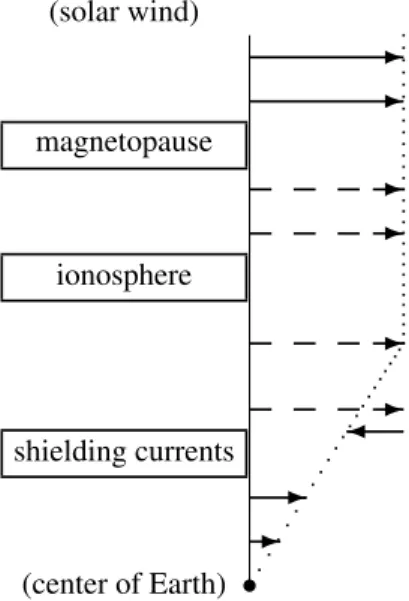
5.3 Linear momentum transfer within the Earth’s interior As long as no non-negligible electric current is crossed while the bounding surface is displaced through the atmosphere and into the Earth’s interior, the total electromagnetic force on the enclosed volume remains unchanged: sunward, equal to[A−1]Fsw1−Fsw0, and balanced by an antisunward me-chanical force that slightly exceeds it in magnitude; the total, net antisunward force no longer equalsFsw, however, but continually decreases as the enclosed mass becomes signifi-cantly less thanME. Within the electrically conducting inte-rior, the diurnally varying perturbations of the external mag-netic field induce currents that shield out the external field; once the bounding surface has been displaced inward of the layer that contains the shielding currents, there is of course no electromagnetic force of external origin, and the mechani-cal force is simply equal to the net acceleration multiplied by the remaining enclosed mass. The integrated Lorentz force on the shielding currents, directed sunward, is the equal and opposite reciprocal force (in the sense discussed in Sects. 2 and 4) to the Lorentz force in the ionosphere; it is opposed by an antisunward mechanical stress, of which a small part is associated with the acceleration of the entire Earth system by the net force exerted on it by the solar wind, and the rest – in balance with the Lorentz force – is the source of the additional linear momentum transported to the ionosphere.
s
✲ ✲ magnetopause
✲ ✲ ionosphere
✲ ✲
shielding currents ✛
✲ ✲ (center of Earth)
(solar wind)
Fig. 4. Same as Fig. 3 but for the case of negligible Lorentz force in the ionosphere.
reciprocal force to the Lorentz force on the Chapman-Ferraro currents), transferring linear momentum to accelerate the en-closed mass. In the region between the shielding currents and the surface of the Earth, where the electromagnetic trans-port of linear momentum does not change appreciably while the enclosed mass decreases with decreasing radial distance, there is a sunward mechanical force (NB sunward when de-fined as force on enclosed volume), corresponding to upward transport of antisunward linear momentum in order to en-force the uniform acceleration of the entire Earth.
5.4 Magnetic gradient force
The electromagnetic force on the Earth arising from all forms of the interaction with the solar wind has in previous dis-cussions (Siscoe, 1966, 2006; Carovillano and Siscoe, 1973; Siscoe and Siebert, 2006) been described as a force on the Earth’s dipole and calculated accordingly from the gradient of the external field at the location of the dipole. In reality, the force is exerted on the shielding currents, the magnetic field of which cancels the external field within the deep inte-rior (including the location of the dipole). The total Lorentz force on the shielding current region can be calculated, analo-gously to the Lorentz force on the ionosphere (Sect. 5.2), by exploiting again the quadratic nature of the Maxwell stress tensor to write the force as the surface integral of the cross terms{dipole×disturbance field}, with the disturbance field now expressed as the sum of the external field and the field of the shielding currents. Hence
FEM(above)=FEM(external)+F>EM(shielding) (18)
FEM(below)=FEM(external)+F<EM(shielding) ,
where “above” or “below” now refers to the bounding sur-face of a volume that includes or does not include, respec-tively, the shielding current region. Since the external field, by definition, is unaffected by the shielding currents, the term
FEM(external) has the same value above or below, given by the standard expression for the force on the dipole exerted by the external field:
FEM(external)=(µ·∇)Bext(0) (19) (µ= dipole moment, r=0 location of dipole). The {dipole×shielding-field}terms above and below are
F>EM(shielding)=0 (20)
F<EM(shielding)= −FEM(external) .
The first line of Eq. (20) can be deduced by noting that the termF>EM(shielding), combined with the{dipole×dipole} and{shielding×shielding}terms (both=0), represents the total Lorentz force on the combined system of dipole (dy-namo) and shielding currents, which vanishes by the corol-lary at the end of Sect. 2; the second line follows, by virtue of Eq. (18), simply from FEM(below)=0, the absence of the electromagnetic force when the external field has been shielded out. The Lorentz force on the shielding current re-gion itself is then given by
FEM(above) − FEM(below) (21)
=F>EM(shielding)−F<EM(shielding)
=(µ·∇)Bext(0)
and is precisely equal to the force that the external field alone, in the absence of shielding currents, would exert on the dipole. The total force is thus unaffected by the pres-ence of shielding (a result that, depending on one’s degree of insight, may or may not be considered obvious), and the answer obtained in previous calculations is correct.
6 Limits to Fukushima’s theorem
A necessary condition for global force balance as described in Sects. 4 and 5 is the penetration of magnetic disturbance fields associated with region 1 currents into the Earth’s in-terior, down to depths where the diurnally varying exter-nal fields are shielded out. This poses a problem because the penetration of these fields below the ionosphere is gen-erally thought to be severely limited by a famous theorem proved by Fukushima (1969), following earlier suggestions by Bostr¨om (1964) and Kern (1966) (for a historical account of the origin of the theorem, see Fukushima, 1985a, part I, Sect. 4).
of Birkeland currents closing via potential (zero-curl) iono-spheric currents (B) plus source-free (zero-divergence) cur-rents confined to the ionosphere (C); the theorem then states that the magnetic disturbance fields of (B) are identically zero below the ionosphere, the contributions from the Birke-land currents being cancelled by those from the potential currents in the ionosphere. The theorem also applies in the case of spherical ionosphere and radial magnetic field lines; this was first mentioned by Fukushima (1971), citing a 1970 conference presentation by Vasyli¯unas (which, however, re-mained unpublished), and was later derived by Fukushima (1985b).
The method used by Fukushima (1969, 1971, 1985b) to derive the theorem is in essence a clever deconstruction into geometrical elements sufficiently simple that the result for each one is evident by symmetry. In Appendix B, I present a purely formal mathematical proof, for both planar and spher-ical geometries. The decomposition, indispensable to the theorem, of the height-integrated horizontal ionospheric cur-rentI into potential and source-free components, proposed by Kern (1966) and extensively used by Vasyli¯unas (1970), can be expressed mathematically as
I =∇τ + ˆr×∇ψ (22) whereτ (θ, φ)andψ (θ, φ)are scalar functions; by continuity of current,
∇2τ = −J· ˆr ≡ −Jr = −JkBˆ · ˆr (23) whereJk is the Birkeland current density at the top of the ionosphere. In the case of nearly vertical magnetic field at low altitudes and of ionospheric conductances independent of latitude and longitude, the potential and the source-free currents are the integrated Pedersen and the height-integrated Hall current, respectively, withτ andψboth pro-portional to the electric potential multiplied by the appropri-ate conductance.
Although the Fukushima theorem does allow penetration of some external disturbance fields below the ionosphere, the fields are those from the source-free (Hall) component of ionospheric currents – from precisely the ionospheric cur-rents that donot couple to the magnetosphere and thus do
notconstitute the ionospheric segment of the region 1 cur-rent system. The penetrating disturbance fields allowed by the theorem induce their own Lorentz force in the shield-ing current region, equal and opposite to the Lorentz force on the source-free currents in the ionosphere; there is no net force on the Earth system, and no direct connection to force balance from solar-wind interaction. Thus, the prob-lem posed by the Fukushima theorem still remains: how is the Lorentz force on the potential (Pedersen) component of the ionospheric currents – the currents that directly couple to the magnetosphere, that according to the theorem produce no ground-level magnetic disturbance – to be matched with the necessary reciprocal Lorentz force?
(A) (B) (C)
Electric
current
✛ ✛
✛ ✛ ✛
✲ ✲
✲
✲ ✲ ✲
✛ ✛
✛
✻ ❄ ✻ ❄
✛
Fig. 5. Simple illustration of Fukushima’s theorem (after Fukushima, 1969, 1985b).
As a first step, I calculate the integrated Lorentz force on just the potential part of the ionospheric currents (first term on the right-hand side in Eq. 22), both to verify that it is indeed non-zero and as input to subsequent force balance ar-guments. The force in thexˆ direction is given by the global integral over the ionosphere
Fx=RE2 Z
dxˆ·I×Bd/c=RE2 Z
d∇τ·Bd× ˆx/c (24) where
Z
d≡ Z
sinθ dθ
Z
dφ
andBd is the dipole field. Withτ (θ, φ)related by Eq. (23) to the radial (Birkeland) currentsJr(θ, φ), Eq. (24) can be transformed into an integral overJr; the calculation is given in Appendix C, with the result
Fx = −
BERE3/2c Z
d Jrsinθsinφ (25) (θ,φin geomagnetic coordinates, with signs appropriate for Earth;BEis the surface field strength at the equator). A sim-ple model for region 1 Birkeland currents (basis for many analytical calculations of magnetospheric convection, e.g., Vasyli¯unas, 1970, 1972) is
Jr =J0sinφ
δ θ−θpc
+δ θ−π+θpc
(26) whereθpcis the colatitude of the polar cap, and the parameter
J0is related to the total currentIoof the region 1 system by
I0=4J0RE2sinθpc. (27)
Inserting Eq. (26) into Eq. (25) gives the force at once as
Fx = −(π BEI0RE/4c)sinθpc≡ −FT , (28) the minus sign indicating that the force is antisunward.
Jr assumed specified by Eq. (26), the results are
Fx(polar cap)= FT n
−2+
sinθpc/ 1+cosθpc 2o
(29)
Fx(low-lat) = FT n
+1−
sinθpc/ 1+cosθpc2 o
(30) the sum of the two giving, as expected,Fx=−FT in agree-ment with Eq. (28).
The results in Eqs. (28), (29), and (30) differ from those of Siscoe (2006), who also assumed the Birkeland current con-figuration of Eq. (26) but treated the ionosphere in the planar approximation (formally, the limit sin2θpc≪1), obtaining (in my notation): Fx(polar cap)=−2FT,Fx(low-lat)=0, hence
Fx(total)=−2FT. In Appendix D, I show that the flat-Earth approximation is the reason for these discrepancies as well as some other paradoxical features.
6.1 Force balance in the idealized geometries
There are two idealized geometries for which Fukushimas’s theorem holds exactly: planar (straight field lines), and spherical (radial field lines). Although these geometries are of course quite inadequate as models for any known exist-ing magnetosphere, situations can be envisaged where they might constitute a reasonable approximation; the radial-field case in particular has been discussed as the extreme limit of a plasma-dominated magnetosphere (Parker and Stewart, 1967). It is instructive to consider how Fukushima’s theorem can be reconciled with force balance in such a case.
In the planar case there is no problem at all: the magnetic field has the same magnitude in the ionosphere as in the mag-netosphere, hence there is no amplification of the Lorentz force — the linear momentum being imparted to the neutral atmosphere is equal to that being extracted from the solar wind.
In the radial-field case, the integrated Lorentz force on the ionosphere is given (Appendix C) by
Fx= −
BERE3/c Z
d Jrsinθsinφ/ (1+ |cosθ|) ,(31) different slightly but not significantly from Fx in Eq. (25), and of course greatly amplified relative to the magnetospheric/solar-wind value. An additional Lorentz force exists, however, in this case: the force exerted by the region 1 disturbance fieldsδBacting on the current sheet in the equatorial plane (separating the oppositely directed radial fields of the two hemispheres). With the radial magnetic field of Eq. (C18), the current density isJ=Iδ(z)where
(4π/c)I= −2BEφˆ(RE/r)2 , (32) and the Lorentz force is given by the integral over the current sheet in the equatorial plane
Fx(eq)= I
dφ
Z
RE
r drxˆ·I×δB/c . (33)
From Eqs. (B1) and (B13),
δB= ∇α× ˆr, (34)
comparison of Eq. (B14) atr=REwith Eq. (22) establishing thatα=(4π/c)τ; then
Fx(eq)=(2BE/c)
I
dφ
Z
RE
(RE/r)2drxˆ·ˆr∂τ/∂φ|θ=π
2 (35)
which can be rewritten, by carrying out the integration over
rand integrating by parts overφ, as
Fx(eq)= +(2BERE/c) I
dφ τθ= π 2, φ
sinφ (36) (the upper limit of ther-integration has been taken nominally as∞). Equation (36) for the Lorentz force integrated over the equatorial current sheet is identical, except for the op-posite sign, with Eq. (C22) for the Lorentz force integrated over the ionosphere (for the case of radial field lines); note that this result is completely general and doesnotdepend on any particular choice (e.g., Eq. 26) of the Birkeland current configuration.
The absence of magnetic perturbations below the iono-sphere in the radial-field-line magnetoiono-sphere, implied by the exact validity of Fukushima’s theorem, is thus possible be-cause the Lorentz force reciprocal to that in the ionosphere is here to be found in the equatorial current sheet; the lin-ear momentum being imparted to the neutral atmosphere is extracted from plasma at the reversal of the radial magnetic field. Antisunward linear momentum is predominantly trans-ported downward, from the current sheet to the ionosphere, by electromagnetic stress, with balancing upward transport by mechanical stress; below the ionosphere there is only a small, purely mechanical stress, needed to exert the force
Fsw on the Earth.
6.2 Fukushima’s theorem in a realistic geometry
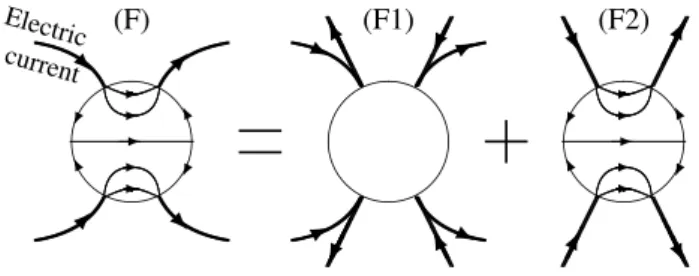
It remains only to verify that system (F1) has the appro-priate value of the Lorentz force. The contributions from the dipole segments are zero becauseJ×B=0. To evaluate the contributions from the radial segments, note that on them
Jr = −Jr(RE, θ, φ) (RE/r)2 (37) where Jr(RE, θ, φ) is the current flowing into the iono-sphere, and the minus sign appears because the current on the radial segment is opposite to the Birkeland current. Then the integrated Lorentz force is
Fx(r)= − Z
d
Z
RE
r2dr Jr xˆ· ˆr× ˆθBθ/c . (38)
WithBθ=−BE(RE3/r3)sinθand xˆ · ˆr× ˆθ=−sinφ, carry-ing out the integration overrgives
Fx(r)= −
BERE3/2c Z
d Jrsinθsinφ (39) which is identical with Eq. (25), including the sign; this again is a general result, independent of any specific model for the Birkeland current configuration. The Lorentz force in the interior is the result of shielding out the perturbation fields which are identical with those of (F1); it can thus be viewed indifferently as the reciprocal force either to the Lorentz force of (F1) or to the real Lorentz force on the ionosphere.
7 Conclusions
As a consequence of the strongly converging geometry of the geomagnetic field lines combined with the condition of current continuity, the Lorentz force on the ionospheric seg-ment of any current system flowing between the ionoasphere and the magnetosphere is greatly amplified relative to the Lorentz force on the magnetospheric or solar-wind segment; the magnetosphere may be said to possess a mechanical ad-vantage over the ionosphere. The forces arising out of the in-teraction with the solar wind are thus much larger within the ionosphere-atmosphere-Earth system than within the magne-tosphere. The total force on the entire system, however, is limited by the rate of extraction of linear momentum from the flow of the solar wind. The large amplified forces must therefore be primarily internal forces between one part of the system and another. Specifically, the antisunward Lorentz force of the region 1 currents in the ionosphere is balanced by a sunward mechanical reaction force of the thermosphere, which is transferred downward through the atmosphere into the Earth’s interior, where it is matched by an antisunward mechanical force balanced by the sunward Lorentz force of the electrical currents that shield out the time-varying exter-nal magnetic fields.
The following are some of the principal implications: 1. The mechanical stresses on the neutral medium that
re-sult from the interaction of the magnetosphere with the
(F) (F1) (F2)
Electric current ✫✪ ✬✩ ✲ ☛ ❑ ❑ ☛ ✲ ✲ ✲ ✲ ✫✪ ✬✩ ✫✪ ✬✩ ✲ ☛ ❑ ❑ ☛ ✲ ✲ ✲ ✲ ❆ ❆ ❆ ❆ ❆ ❆ ✁ ✁ ✁✁✁✁ ✁✁✁✁✁✁ ❆ ❆❆ ❆ ❆❆ ❆ ❆❑ ☛ ✁ ✁☛ ❑ ❥ ✯ ✯ ❥ ❘ ✒ ✒ ❘ ❆ ❆ ❆ ✁ ✁ ✁ ✁✁✁ ❆ ❆❆ ❆ ❆ ❆ ✁ ✁ ✁ ✁✁✁ ❆ ❆❆ ❯ ✁✁✕ ✕ ❆❆❯
Fig. 6. Curvature effect in Fukushima’s theorem (after Fukushima, 1985b).
solar wind are not confined to the thermosphere but ex-tend also into the atmosphere and into that part of the Earth’s interior into which any diurnally varying mag-netic disturbances can penetrate.
2. The forces involved can be much larger than the net force exerted by the solar wind on the entire Earth sys-tem (although they still are utterly negligible compared to with forces involved in dynamics of the atmosphere, let alone of the solid Earth).
3. Except in the case of very weak region 1 currents (in the quantitative sense discussed by Siscoe and Siebert, 2006), the total magnetic force on the Earth’s interior is sunward; it is slightly overbalanced by an antisunward mechanical force, the difference being equal to the net force exerted by the solar wind.
4. The magnetic disturbance fields in the Earth’s inte-rior that result from the region 1 currents play an es-sential role in maintain stress balance; hence limits on them imposed by Fukushima’s theorem necessarily are of restricted applicability (the requisite deviations from the ideal theorem have been identified already by Fukushima, 1985b).
Appendix A
Acceleration of center of mass
Introduce the center of massRthrough the definitions
MR≡ Z
d3r ρr M≡ Z
d3r ρ (A1)
Noting thatr andtare independent variables, we have
dM/dt= Z
d3r ∂ρ/∂t= − Z
dS·ρV (A2)
and
d (MR) /dt= Z
d3rr∂ρ/∂t= Z
d3r ρV− Z
where in both equations the second expression follows from the mass continuity equation, plus an integration by parts in Eq. (A3). Differentiating once more with respect to t and rearranging, we have
(d/dt )
Z
d3rρV=d2(MR) /dt2+ Z
dS·(∂ρV/∂t )r (A4) which can be manipulated into the form
(d/dt )
Z
d3rρV =M d2R/dt2 (A5) + 2(dM/dt ) (dR/dt )+
Z
dS·(∂ρV/∂t ) (r−R)
from which Eq. (12) follows.
Appendix B
Formal derivation of Fukushima’s theorem
Represent the disturbance magnetic field (notthe total field) by Euler potentials
B= ∇α× ∇β; (B1)
then the current density is given by (ignoring the factor 4π/c
in Gausian orµ0in SI units)
∇×B=∇α∇2β+(∇β·∇)∇α−∇β∇2α−(∇α·∇)∇β (B2) For the planar case as in Fig. 5 (vertical direction taken aszˆ), choose
α=α(x, y) β =β(z) (B3)
which simplifies Eq. (B2) to
∇ ×B= ∇α∇2β− ∇β∇2α . (B4)
Now require
∇2β=d2β/dz2=δ(z) (B5)
β=0 forz <0 (B6)
where δ(z) is merely an idealization of a sharply peaked function; Eqs. (B5) and (B6) are satisfied if
∇β = ˆzH (z) (B7)
withH the function defined by H (z)=1 x >0
H (z)=0 x <0
(Heaviside unit function). From Eq. (B4), the current density is then given by
∇ ×B=δ(z)∇α− ˆzH (z)∇2α , (B8) which describes a system identical with (B) in Fig. 5: vertical currents in the spacez>0 (magnetosphere), closed by a curl-free current atz=0 (ionosphere). Condition (B6) together
with (B1) implies that the disturbance magnetic field of this system vanishes in the spacez<0 (below the ionosphere), which is Fukushima’s theorem.
An analogous calculation can be carried out for the spher-ical case by choosing α=α(θ, φ), β=β(r). The cross-gradient terms in Eq. (B2) are now, unlike the planar case, no longer zero; they can, however, be written as
(∇β· ∇)∇α= −(1/r) (dβ/dr)∇α= −(∇α· ∇)∇β(B9) which simplifies Eq. (B2) to
∇ ×B= ∇αh∇2β−(2/r) (dβ/dr)i− ∇β∇2α . (B10) With the requirements
∇2β−(2/r) (dβ/dr)=d2β/dr2=δ(r−RE) (B11)
β =0 forr < RE (B12)
satisfied if
∇β = ˆrH (r−RE) , (B13)
the current density is given by
∇ ×B=δ(r−RE)∇α− ˆrH (r−RE)∇2α , (B14) the spherical counterpart of (B) in Fig. 5: a system of radial currents atr>REclosed by a curl-free current atr=RE, with vanishing disturbance magnetic field forr<RE. (Note: gen-eralizing the theorem even further is not possible, apparently, as the method used here does not seem to work when applied to any other
Appendix C
Calculation of ionospheric Lorentz force
Equation (24) may be written as
Fx =RE2 Z
dQ· ∇τ (C1)
where
Q≡Bd× ˆx/c . (C2) Only theθˆ andφˆ components ofQappear in Eq. (C1); they may be separated into curl-free and divergence-free parts by writing
Q− ˆrQr = ∇G+ ˆr× ∇H/r2 (C3) (Qr≡Q· ˆr), whereG(θ, φ)andH(θ, φ)are scalar functions;
r=RE throughout this calculation. Integrating by parts now transforms Eq. (C1) into
Fx = Z
d h∇ · G∇τ+τ rˆ× ∇H
noting that the integral of the divergence over the entire sphere vanishes, we have
Fx= − Z
dG∇2τ = Z
dGJr. (C5)
To derive the functionG, take the divergence of Eq. (C3):
1/r2∇2G= ∇ · Q− ˆrQr . (C6) Noting that from Eq. (C2)
∇ ·Q= ˆx· ∇ ×Bd/c=0 (C7)
andQr∼1/r3, we have
∇2G=rQr =r·Bd× ˆx/c= ˆx×µ·r/r3c≡U . (C8) The Laplacian has been written as∇2
to emphasize thatGis a function ofθ,φonly. The direct solution of Eq. (C8) for G, straightforward but tedious, can be avoided by noting that the expressionUis the scalar potential of a dipole field (with momentxˆ×µ/c), hence its (3-D) Laplacian is zero, which implies that
∇2U= −1/r2(∂/∂r) r2(∂U/∂r)= −2U/r2. (C9) Comparing Eq. (C9) with Eq. (C8), we have
G= −RE2U/2= − ˆx×µ· ˆr/2 (C10) = −BERE3/2c
sinθsinφ ,
which inserted into Eq. (C5) gives Eq. (28) of the main text. To calculate the force integrated over only a portion of the entire sphere, the boundary contribution from the divergence term in Eq. (C4) must be included. Specifically, under the assumption (Eq. 26) of Birkeland currents non-zero only at the polar cap boundaries, the forces on the polar-cap and the non-polar-cap regions are given by
Fx(polar cap)=
2/RE2 I
dφ Kθpc−, φ (C11)
Fx(low-lat) = −
2/RE2 I
dφKθpc+, φ (C12) K≡G sinθ (∂τ/∂θ )−τ (∂H/∂φ)
(the factor 2 comes from including both hemispheres). The function H can be derived from Eqs. (C3) and (C10), with use of the relations∇(a·r)=afor any constanta and
Q−ˆrQr=ˆr×(Q׈r):
H=(3/2)µ·ˆrxˆ·ˆr=−3BERE3/2c
sinθcosθcosφ .(C13) Solving Eq. (23) forτ, withJrgiven by Eq. (26), we have
τ =RE2J0sinφsinθ/ (1+ |cosθ|)
θ < θpc π−θpc < θ
=RE2J0sinφ 1− |cosθpc|/sinθ
θpc< θ < π−θpc . (C14)
Equations (C11–C12) then give
Fx(polar cap)= −FT 1+3 cosθpc/ 1+cosθpc (C15)
Fx(low-lat) = −FT −2 cosθpc/ 1+cosθpc (C16)
FT =
π BERE3J0/c
sin2θpc,
equivalent to Eqs. (29–30) of the main text by virtue of Eq. (27) and the identity
(1−cosθ ) / (1+cosθ )=[sinθ/ (1+cosθ )]2 . (C17) For the case of radial field lines discussed in Sect. 6.1,Bdin Eq. (C2) is replaced by
B= −ˆrBEsign(cosθ ) (C18)
(the magnetic flux through a hemisphere is the same as for the dipole field with equatorial field strength BE). Then
Qr=0 everywhere, but∇×B and hence also∇·Qare non-zero at the singular pointθ=π/2 (field reversal), with the result that in place of Eq. (C8) we have
∇2G=(2BERE/c) sinφ δ (cosθ ) (C19) which has the solution
G= −BERE3/c
sinθsinφ/ (1+ |cosθ|) , (C20) the only change from Eq. (C10) being the replacement of a factor 2 in the denominator by(1+|cosθ|). Instead of insert-ing thisGinto Eq. (C5), however, it is simpler in this case to derive an alternative expression forFx, by using a different integration by parts to transform Eq. (C1) into
Fx = − Z
d τ∇2G (C21)
and then substituting from Eq. (C19) to obtain
Fx = −(2BERE/c) I
dφ τθ=π 2, φ
sinφ (C22)
which can be compared directly with the force calculated in Sect. 6.1.
Appendix D
The paradoxes of flatland
plane which preserves the form of some of the key equa-tions of magnetosphere-ionosphere coupling theory: the (po-lar) stereographic projection, in which any point P on the surface of the sphere is projected onto the plane tangent to the north pole by drawing a straight line from the south pole through P. The coordinates (θ,φ) on the surface of the sphere are mapped to cylindrical coordinates (R,φ) on the plane, withφunchanged andRrelated toθby
R/RE =2 sinθ/ (1+cosθ ) . (D1)
Th equator maps toR=2REand the south pole toR→ ∞; the flat-Earth approximation near the north pole is obtained in the limitR≪RE (or equivalently sinθ≪1).
The 2-D Laplacian ∇2
in (θ,φ) coordinates transforms into the 2-D Laplacian in (R,φ) coordinates, multiplied by the factor [2/(1+cosθ )]2=[1+(R/2R
E)2]2. The current continuity Eq. (23) is thus unchanged in form, as is Eq. (22). By direct transformation it can be shown that Eqs. (C1–C5) and (C11–C12) remain valid when expressed in (R,φ) coor-dinates. The functionsG,Hbecome in these coordinates
G= −BERE2/2c
Rsinφ {1/ (1+X)} (D2) H= −3BERE2/2c
Rcosφ n(1−X) / (1+X)2o (D3)
X≡(R/2RE)2 ;
the factors enclosed in{ }reduce to±1 in the flat-Earth ap-proximation. It is now apparent why calculating a global force correctly is intrinsically impossible in this approxima-tion: to obtain a global force, the integrals must be taken over the entire plane, but as long as the factors in{ }remain ap-proximated by±1,G andHboth diverge for largeR/RE. (By contrast, for calculations relating the ionospheric elec-tric potential to the Birkeland current distribution, departures from the flat-Earth approximation involve changes only of field magnitude and inclination, which remain bounded over the entire plane.)
As noted already in Sect. 6, calculations by Siscoe (2006) in the flat-Earth approximation give the correct value−2FT (in the limit sin2θpc≪1) for the integrated Lorentz force on the polar cap, but not on the low-latitude region; the correct value for the latter is+FT, whereas Siscoe (2006) obtains zero, finding that the sunward Lorentz force on the Peder-sen currents just equatorward of the polar cap is balanced by the force on the return currents farther away. The physical reason for the discrepancy is that the return currents on the sphere occupy a smaller effective area than on the plane and are also subject to a smaller vertical geomagnetic field. The zero value for the flat-Earth calculation is in fact unique to the boundary condition implicitly assumed by Siscoe (2006),
τ→0 atR→∞. If one takes instead as the boundary condi-tion∂τ/∂R=0 at some fixed (large)R=R1, which is physi-cally more realistic (it corresponds to the assumption of zero current acrossR=R1, e.g., the equator), one obtains the inte-grated Lorentz force on the low-latitude region=−2FT for
anyvalue ofR1(the physical reason is that the return cur-rents have been enhanced even further by their confinement toR≤R1).
Acknowledgements. I am grateful to G. L. Siscoe for useful discus-sions.
Topical Editor I. A. Daglis thanks A. Richmond and another referee for their help in evaluating this paper.
References
Bostr¨om, R.: A model of the auroral electrojets, J. Geophys. Res., 69, 4983–4999, 1964.
Carovillano, R. L. and Siscoe, G. L.: Energy and momentum theo-rems in magnetospheric dynamics, Rev. Geophys. Space Phys., 11, 289–353, 1973.
Fukushima, N.: Equivalence in ground magnetic effects of Chapman-Vestine’s and Birkeland-Alfv´en’s electric current-systems for polar magnetic storms, Rep. Ionos. Space Res. Japan, 23, 219–227, 1969.
Fukushima, N.: Electric current systems for polar substorms and their magnetic effect below and above the ionosphere, Radio Sci., 6, 269–275, 1971.
Fukushima, N.: Contribution to two selected subjects in Geomag-netism: Electric currents in the ionosphere-magnetosphere, and archaeo-secular variation of geomagnetic field, in: Prospect and Retrospect in Studies of Geomagnetic Field Disturbances, edited by: Nishida, A., Kokubun, S., Iijima, T., Kamide, Y., and Tamao, T., 1–18, Geophysical Research Laboratory, University of Tokyo, 1985a.
Fukushima, N.: Ground magnetic effect of field-aligned currents connected with ionospheric currents: Fundamental theorems and their applications, in: Prospect and Retrospect in Studies of Geo-magnetic Field Disturbances, edited by: Nishida, A., Kokubun, S., Iijima, T., Kamide, Y., and Tamao, T., 19–39, Geophysical Research Laboratory, University of Tokyo, 1985b.
Iijima, T. and Potemra, T. A.: The amplitude distribution of field-aligned currents at northern high latitudes observed by Triad, J. Geophys. Res., 81, 2165–2174, 1976.
Kern, J. W.: Analysis of polar magnetic storms, J. Geomag. Geo-electr., 18, 125–131, 1966.
Landau, L. D. and Lifshitz, E. M.: Fluid Mechanics, Pergamon Press, London, 1959.
Mead, G. D. and Beard, D. B.: Shape of the geomagnetic field solar wind boundary, J. Geophys. Res., 69, 1169–1179, 1964. Parker, E. N. and Stewart, H. A.: Nonlinear inflation of a magnetic
dipole, J. Geophys. Res., 72, 5287–5293, 1967.
Price, A. T.: Electromagnetic induction within the Earth, in: Physics of Geomagnetic Phenomena, Vol. 1, edited by: Mat-sushita, S. and Campbell, W. H., 235–298, Academic Press, New York, 1967.
Rossi, B. and Olbert, S.: Introduction to the Physics of Space, McGraw–Hill, New York, 1970.
Siscoe, G. L.: A unified treatment of magnetospheric dynamics with applications to magnetic storms, Planet. Space Sci., 14, 947–967, 1966.
Siscoe, G. L.: Solar system magnetohydrodynamics, in: Solar-Terrestrial Physics, edited by: Carovillano, R. L. and Forbes, J. M., 11–100, D. Reidel Publishing Co., Dordrecht–Holland, 1983.
Siscoe, G. L.: Global force balance of region 1 cur-rent system, J. Atmos. Solar-Terr. Phys., 68, 2119–2126, doi:10.1016/j.jastp.2006.09.001, 2006.
Siscoe, G. L., Crooker, N. U., and Siebert, K. D.: Transpo-lar potential saturation: Roles of region 1 current system and solar wind ram pressure, J. Geophys. Res., 107(A10), 1321, doi:10.1029/2001JA009176, 2002.
Siscoe, G. L. and Siebert, K. D.: Bimodal nature of solar wind-magnetosphere-ionosphere-thermosphere coupling, J. Atmos. Solar-Terr. Phys., 68, 911–920, doi:10.1016/j.jastp.2005.11.012, 2006.
Vasyli¯unas, V. M.: Mathematical models of magnetospheric con-vection and its coupling to the ionosphere, in: Particles and Fields in the Magnetosphere, edited by: McCormack, B. M., 60– 71, D. Reidel Publishing Co., Dordrecht–Holland, 1970.
Vasyli¯unas, V. M.: The interrelationship of magnetospheric pro-cesses, in: The Earth’s Magnetospheric Processes, edited by: McCormack, B. M., 29–38, D. Reidel Publishing Co., Dordrecht–Holland, 1972.
Vasyli¯unas, V. M.: Plasma distribution and flow, in: Physics of the Jovian Magnetosphere, edited by: Dessler, A. J., 395–453, Cam-bridge University Press, N.Y., 1983.
Vasyli¯unas, V. M.: Contribution to “Dialog on the relative roles of reconnection and the ’viscous’ interaction in providing solar-wind energy to the magnetosphere,” in: Magnetotail Physics, edited by: Lui, A. T. Y., 411–412, The Johns Hopkins Univer-sity Press, Baltimore, 1987.