www.hydrol-earth-syst-sci.net/19/3217/2015/ doi:10.5194/hess-19-3217-2015
© Author(s) 2015. CC Attribution 3.0 License.
Impacts of climate change on temperature, precipitation
and hydrology in Finland – studies using bias corrected
Regional Climate Model data
T. Olsson1, J. Jakkila2, N. Veijalainen2, L. Backman1, J. Kaurola1, and B. Vehviläinen2
1Finnish Meteorological Institute, Erik Palménin aukio 1, 00101, Helsinki, Finland
2Freshwater Centre, Finnish Environment Institute, Mechelininkatu 34a, P.O. Box 140, 00251, Helsinki, Finland Correspondence to:T. Olsson ([email protected])
Received: 19 January 2015 – Published in Hydrol. Earth Syst. Sci. Discuss.: 3 March 2015 Revised: 11 June 2015 – Accepted: 23 June 2015 – Published: 24 July 2015
Abstract.Assessment of climate change impacts on climate and hydrology on catchment scale requires reliable informa-tion about the average values and climate fluctuainforma-tions of the past, present and future. Regional climate models (RCMs) used in impact studies often produce biased time series of meteorological variables. In this study bias correction (BC) of RCM temperature and precipitation for Finland is carried out using different versions of the distribution based scal-ing (DBS) method. The DBS-adjusted RCM data are used as input of a hydrological model to simulate changes in dis-charges of four study catchments in different parts of Fin-land. The annual mean discharges and seasonal variation simulated with the DBS-adjusted temperature and precipi-tation data are sufficiently close to observed discharges in the control period 1961–2000 and produce more realistic projections for mean annual and seasonal changes in dis-charges than the uncorrected RCM data. Furthermore, with most scenarios the DBS method used preserves the temper-ature and precipitation trends of the uncorrected RCM data during 1961–2100. However, if the biases in the mean or the standard deviation of the uncorrected temperatures are large, significant biases after DBS adjustment may remain or tem-perature trends may change, increasing the uncertainty of cli-mate change projections. The DBS method influences espe-cially the projected seasonal changes in discharges and the use of uncorrected data can produce unrealistic seasonal dis-charges and changes. The projected changes in annual mean discharges are moderate or small, but seasonal distribution of discharges will change significantly.
1 Introduction
Climate in Finland is boreal with temperate and sub-arctic features and four distinct seasons (Castro et al., 2007; Jylhä et al., 2009a). Winters are mostly cold and snowy and sum-mers rather short, cool and rainy. Precipitation is moderate in all seasons. Hydrology in Finland is characterized by sea-sonal variation with snow accumulation and low flow dur-ing winter, snowmelt with runoff peak in sprdur-ing, another low flow season in summer and increasing runoffs towards au-tumn. Climate change is expected to significantly influence the hydrology in Finland. Climate zones are expected to shift towards the north during this century, and the prevailing cli-mate type will become more temperate and wet (Jylhä et al., 2009a). According to Jylhä et al. (2009b) annual mean temperature is likely to increase by 3–6◦C by the end of this
due to decreased snow accumulation (Vehviläinen and Hut-tunen, 1997; Veijalainen et al., 2010). The changes in river discharge and lake water levels will cause adaptation needs in water power production, flood protection and lake regula-tion (Veijalainen, 2012).
Regional and local climate change scenarios are needed for assessments of climate change impacts on hydrology and other sectors in Finland. The spatial resolution of global cli-mate models (GCM) (100–300 km) is insufficient to simu-late regional scale events that are needed to capture differ-ent weather phenomena in a catchmdiffer-ent scale. Projections of GCMs can be dynamically downscaled with regional climate models (RCMs) to scales of 25–50 km, which represents the Finnish catchment scales better. Though nested models are more computationally demanding, dependent on GCM forc-ing and need detailed surface data, they are able to produce more detailed information on temporal and spatial scales than GCMs (Hewitson and Crane, 1996). This information is nec-essary when RCM data are used as input for impact models such as hydrological models.
Although increased horizontal resolution can improve the simulation of regional and local climate features, RCMs still produce biases in the time series of climate variables (Chris-tensen et al., 2008; Rauscher et al., 2010). RCMs are found to have lower skill to reproduce temperature and precipita-tion in colder regions (Teutschbein and Seibert, 2012) and have difficulties to reproduce realistic values near the coast line and lakes in Finland (Jylhä et al., 2009b). Hydrologi-cal simulations using the RCM data as direct input are sen-sitive to RCM biases (Wood et al., 2004), and especially re-gions such as Finland are sensitive to temperature bias, where seasonal snowpack causes a time shift in runoff generation (Wood et al., 2004; Veijalainen et al., 2012). Therefore, an efficient bias correction (BC) method for both precipitation and temperature should be applied to the RCM data.
Several approaches are available for adjusting RCM vari-ables; these can be divided into delta change (DC) and BC methods. The DC approach adjusts observations with the RCM climate change signal, whereas the BC approach ad-justs the daily RCM simulated variables based on the dif-ference between observed and simulated climate in the con-trol period. Compared to the DC method the BC approach usually better preserves the future variability in temperature and precipitation produced by the RCMs, enables represen-tation of complex changes in climate related to changes in mesoscale weather conditions and enables transient scenar-ios instead of comparison between time slices (Graham et al., 2007; Lenderink et al., 2007; Beldring et al., 2008; Yang et al., 2010). Bias correction methods have been proved to improve daily mean, standard deviation (SD), and distribu-tion of the RCM temperature and precipitadistribu-tion when com-pared to observed climate statistics (e.g. Yang et al., 2010; Teutschbein and Seibert, 2012; Räisänen and Räty, 2013; Räty et al., 2014).
In this paper, bias corrected RCM data sets of precipita-tion and temperature covering the area of Finland are pro-duced. Two versions of a distribution based bias correction method are evaluated for temperature and precipitation. In addition, a simple mean bias correction is applied for daily wind speed and specific humidity, which are used in simu-lation of lake evaporation in the hydrological model. These bias corrected values are then used as input of the hydrolog-ical model to simulate discharges and their changes due to climate change in selected catchments. The goal is to eval-uate the DBS method in climate change impact studies of river discharges in Finland. This article focuses on annual and seasonal mean values, while the second part of the study in a separate paper will focus on extremes, especially heavy precipitation and floods, and their changes.
2 Materials and methods
In this study, climate scenarios from RCMs are first bias cor-rected using observations of temperature, precipitation, wind speed and humidity and then used to produce hydrological scenarios for the study catchments (Fig. 1).
2.1 Study catchments
Four catchments located in different parts of Finland were se-lected as study catchments (Fig. 2). These represent different hydrological regions in Finland. Loimijoki (Maurialankoski observation station, catchment area 2650 km2; lake percent-age 3.1) is a medium sized river with high proportion of culti-vated area on clay soils. Nilakka (catchment area 2160 km2; 18 % lake percentage) and Lentua (2050 km2; 13 %) obser-vation stations are located at lake outlets in central Finland characterized by numerous lakes. Ounasjoki (Marraskoski observation station, 12 300 km2; 2.6 %) is a large river in northern Finland (Fig. 2) (Korhonen and Kuusisto, 2010). All the study catchments have long water level and discharge ob-servation series, the longest from 1912 onwards (Lentua) and the shortest from 1935 onwards (Loimijoki).
sum-Regional Climate Models Observations Bias correction
(1961-2000)
Daily precipitation (1961-2000, 2001-2100)
Monthly precipitation
Drizzle remove Daily precipitation
(1961-2000)
Monthly precipitation
Drizzle remove
Precipitation with DBS
2 Gamma
Daily temperature (1961-2000) All
days
Daily mean and SD
Fourier smoothing 15-day moving mean
Temperature With DBS
Gaussian 1 Gamma
Daily temperature (1961-2000, 2001-2100) All
days Wet days
Dry days
Daily mean and SD
Fourier smoothing 15-day moving mean
Climate projection (2001-2100)
WSFS Hydrological model Hydrological scenarios
for 140 years
Wind and Specific humidity (1961-2000, 2001-2100)
Monthly mean Wind and
Specific humidity Wind and
Specific humidity (1961-2000)
Monthly mean correctionMean Wet
days Dry days
W/D Gaussian
Figure 1.Schematic presentation of application procedure used in this study for hydrological modelling of climate change impact with bias corrected RCM data.
mer and autumn or rains with snowmelt in winter may cause major floods as well.
2.2 Observations and RCM data
Bias corrections were calculated for the entire Finland in-cluding transboundary watershed areas in Norway, Sweden and Russia. The gridded data sets needed for the bias cor-rection were calculated using observations from approxi-mately 190 stations with daily temperature measurements at 2 m height and 250 stations with daily precipitation mea-surements from the Finnish Meteorological Institute (FMI). Additional observations from 11 temperature and 16 pre-cipitation observation stations in Norway, Sweden and Rus-sia were provided by the Norwegian Meteorological Insti-tute, the Swedish Meteorological and Hydrological Institute (SMHI) and the Hydrometeorological Centre of Russia. Ob-servations from 1961 to 2000 were used although the obser-vation network varies during this period.
Gauge precipitation observations especially for snowfall contain various systematic measurement errors (Førland et al., 1996; Taskinen, 2015), which need to be corrected be-fore they can be used for bias correction of RCM data. The
correction of precipitation measurements consisted of the ex-posure method for aerodynamic correction as well as wet-ting and evaporation corrections (Taskinen, 2015). The areal values of the meteorological observations are calculated for each sub-basin of the hydrological model from three clos-est observation stations by inverse distance weighting taking into account the elevation differences. The areal values were converted to the same regular 0.25◦lat×0.25◦long grid as the
RCM data.
The observations of relative humidity at 2 m and wind speed at 10 m are used in the simulation of lake evaporation, which is an important hydrological variable for catchments in the lake area. The areal values are calculated in a similar way as temperature and precipitation and the effect of fetch to the wind speed on a lake is calculated as in Resio and Vin-cent (1977).
! (
! (
! ( !
(
Lentua
Nilakka Ounasjoki
Loimijoki
Figure 2.Map of the study catchments.
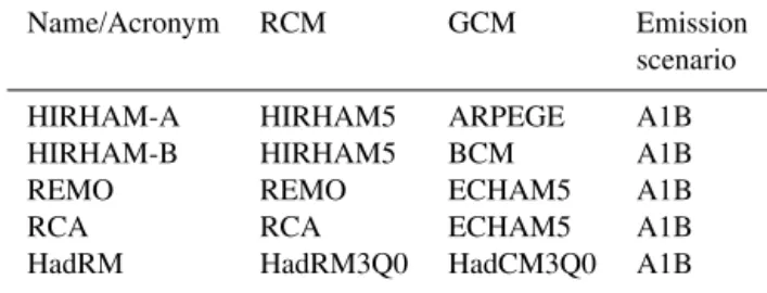
Table 1.Regional climate model (RCM) data used in this study.
Name/Acronym RCM GCM Emission scenario HIRHAM-A HIRHAM5 ARPEGE A1B HIRHAM-B HIRHAM5 BCM A1B REMO REMO ECHAM5 A1B RCA RCA ECHAM5 A1B HadRM HadRM3Q0 HadCM3Q0 A1B
HIRHAM5 is a combination of the HIRLAM (High Resolution Limited Area Model) and ECHAM; REMO is the Max Planck Institute’s REgional MOdel; RCA is the Rossby Center Regional Atmospheric Model; HadRM3Q0 is the Hadley Centre Regional Model, version 3 (normal sensitivity);
ARPEGE is the Action de Recherche Petite Echelle Grande Echelle; BCM is the Bergen Climate Model; ECHAM5 is the European Centre Hamburg model, version 5; HadCM3Q0 is the Hadley Centre Coupled Model, version 3 (normal sensitivity).
project’s research team 3 database (ensemblesrt3.dmi.dk; van der Linden and Mitchell, 2009). The GCMs were run under historic (1961–2000) and with A1B scenario (2001–2100) forcing. The GCM output was then used as boundary con-ditions to force RCMs over a common European domain in a regular 0.25◦lat×0.25◦long grid (van der Linden and
Mitchell, 2009).
Figure 3. Procedure of the distribution based mapping. Upper panels for temperature adjustment and lower panels for precipita-tion (pr) adjustment. For temperature, Gaussian adjustment without wet–dry state separation (left) and with wet–dry separation (right) is shown. For precipitation, gamma adjustment with single gamma (left) and double gamma divided at 95th percentile (right) is shown. (1) Locate the cumulative probability value of RCM simulated daily temperature/precipitation. (2) Locate the observed tempera-ture/precipitation value corresponding the same cumulative proba-bility value as in (1). (3) This value is used as corrected value for RCM simulation.
2.3 Bias correction methods
The distribution based scaling (DBS) method described, e.g., in Yang et al. (2010) and Teutschbein and Seibert (2012) was used to scale temperature and precipitation time series to better represent observed distributions. The correction pro-cedures using cumulative distribution functions (CDFs) are shown in Fig. 3. In this study CDFs are constructed on a daily basis for temperature and for all days with certain months for precipitation. The method of maximum likelihood is used to estimate distribution parameters.
Temperature (T) is described by a Gaussian (normal) dis-tribution with daily mean (µ) and standard deviation (σ). The DBS approach for temperature included four steps: (1) to take into account the dependence between precipitation and temperature, the temperature data were divided into wet and dry days resulting in two sets of parameters; (µw,σw) for
deviation for each grid point were then used to calculate the daily (d) CDFs for observations (µobs,σobs) and RCMs (µcontr,σcontr) for the control period (Fig. 3). DBS parame-ters for the control period were used also to adjust the sce-nario (scen) runs. DBS procedure expressed in terms of the Gaussian CDF without wet–dry separation:
Tcontr(d)=F−1
F Tcontr(d) µcontr, σ 2
contr µobs, σ
2 obs
, (1) Tscen(d)=F−1
FTscen(d)
µcontr, σ
2
contr µobs, σ
2 obs
. (2) DBS procedure expressed in terms of Gaussian CDF with wet–dry separation:
Tcontr, w–d(d)=F−1
·FTcontr, w–d(d)
µcontr, w–d, σ 2
contr, w–d µobs, w–d, σ 2 obs, w–d
, (3) Tscen, w–d(d)=F−1
·FTscen, w–d(d)
µcontr, w–d, σ 2
contr, w–d µobs, w–d, σ 2 obs, w–d
. (4) For precipitation (P) single and double gamma distributions were used in four steps. In contrast to Yang et al. (2010) where the DBS parameters (shape α and scale β) were estimated seasonally, we estimated DBS parameters on a monthly basis. Single CDF for certain month is used for the whole time slice (1961–2000). Also seasonally optimized pa-rameters were tried out, but these produced too high monthly precipitation sums for Finland (not shown) and thus were not used. (1) For both distributions, excessive drizzle days in the RCM data were first removed by defining a cut-off value (Pth,contr,m)that reduced the percentage of wet days in the RCMs to that of the observations on a monthly (m) ba-sis. In this study only days with observed precipitation larger than 0.1 mm (Pth,obs,m)were considered wet days, and the rest dry days. A monthly precipitation threshold value for each RCM control run (Pth,contr,m)was then set to the cut-off value so that the percentage of RCM simulated and observed wet days matched (Eq. 5). Due to the stationary assumption the same threshold value was used to reduce the drizzle days for a future period to enable the scenario run to have dif-ferent wet day frequency than the control run (Eq. 6). Pre-cipitation amounts smaller than the threshold value were not redistributed to the remaining wet days.
Pcontr(d)=
(
0, if Pcontr(d) < Pth, contr,m Pcontr, otherwise
(5)
Pscen(d)=
(
0, if Pscen(d) < Pth, contr,m Pscen, otherwise
(6)
(2) The remaining daily precipitation was adjusted to match the observed frequency distribution using single gamma dis-tribution (Eq. 7). (3) To better capture the extreme precip-itation events a double gamma distribution was also used, then the observed and RCM generated precipitation distri-butions were separated into two by the 95th percentile of
CDF (Pobs,95th,Pcontr,95th), resulting into two sets of parame-ters: (α1,β1) for below the 95th percentile precipitation and (α2,β2) above it. (4) These monthly parameters for each grid point were then used to calculate the CDFs for observations (αobs,βobs) and RCMs (αcontr,βcontr) during the control
pe-riod (Eqs. 9, 10; Fig. 3). Monthly DBS parameters for the control period and the 95th percentile threshold (Pcontr,95th)
were also used for the scenario (scen) runs (Eqs. 8, 11, 12). The DBS procedure expressed in terms of single gamma CDF:
Pcontr(d)=F−1
· F Pcontr(d)|αcontr,m, βcontr,m
|αobs,m, βobs,m
, (7) Pscen(d)=F−1
· F Pscen(d)|αcontr,m, βcontr,m
|αobs,m, βobs,m
, (8) The DBS procedure expressed in terms of double gamma CDF:
Pcontr,1(d)=F−1
· F Pcontr(d)|αcontr1,m, βcontr1,m
|αobs1,m, βobs1,m
,
if Pcontr(d) < Pcontr,95th(m), (9)
Pcontr,2(d)=F−1
· F Pcontr(d)|αcontr2,m, βcontr2,m|αobs2,m, βobs2,m,
if Pcontr(d)≥Pcontr,95th(m), (10)
Psken, 1(d)=F−1
· F Pscen(d)|αcontr1,m, βcontr1,m|αobs1,m, βobs1,m, if Pscen(d) < Pcontr,95th(m), (11)
Psken,2(d)=F−1
· F Pscen(d)|αcontr2,m, βcontr2,m
|αobs2,m, βobs2,m
,
if Pscen(d)≥Pcontr,95th(m). (12)
Wind speed and specific humidity of the RCM data were cor-rected by adding the monthly mean differences between the observations and the RCMs. The same corrections were used in the scenario periods. Since the wind speed and specific humidity affect only the calculation of lake evaporation in the hydrological model, it is assumed that this simple bias correction works sufficiently well to achieve corresponding water level and discharge distribution as with observed input variables.
2.4 Hydrological model and modelling approaches
(e.g. Veijalainen et al., 2012; Jakkila et al., 2014; Hut-tunen et al., 2015). The conceptual rainfall–runoff model in the WSFS is based on the HBV (Hydrologiska Byråns Vattenbalansavdelning) model structure developed at SMHI (Bergström, 1976), but the models differ from each other, e.g., in the river routing, catchment description and in some process models such as the snow model (Vehviläinen, 1992; Vehviläinen et al., 2005). HBV-type models have been used in several climate change impacts studies in different parts of the world (e.g. Steele-Dunne et al., 2008; van Pelt et al., 2009), most commonly in Scandinavia (e.g. Andréasson et al., 2004; Beldring et al., 2008)
The WSFS hydrological model consists of small sub-basins, numbering over 6000 in Finland with an average size of 60 km2(20–500 km2) (Vehviläinen et al., 2005). The wa-ter balance is simulated for each sub-basin, and sub-basin are connected to produce the water balance and simulate water storage and transfer in the river and lake network within the entire catchment. The sub-models in WSFS include a pre-cipitation model calculating areal value and form for precip-itation, a snow accumulation and melt model based on the temperature-index (degree-day) approach, a rainfall–runoff model with soil moisture, sub-surface and groundwater stor-ages, and models for lake and river routing.
The WSFS was calibrated against water level, discharge and snow line water equivalent observations from 1981 to 2012. The Nash–Sutcliffe efficiency criterionR2(Nash and Sutcliffe, 1970) for the control period 1961–2000 in the four case study catchments was 0.78 for Loimijoki, 0.80 for Ni-lakka, 0.87 for Lentua and 0.87 for Ounasjoki. TheR2 val-ues within the calibration period 1981–2000 are considerably better than in the validation period 1961–1980: 0.84 and 0.71 for Loimijoki, 0.91 and 0.68 for Nilakka, 0.92 and 0.81 for Lentua and 0.87 and 0.88 for Ounasjoki, respectively, for calibration and validation periods. The reasons for remark-ably lower values in the validation period are the possible changes in rating curves in Loimijoki and Nilakka and the change of the rain station gauges from Wild to Tretjakov-type gauges. The measurement errors for different gauge types are done separately (Taskinen, 2015), but the uncertainty range of wind effect on snowfalls is much larger for Wild than Tret-jakov.
3 Results
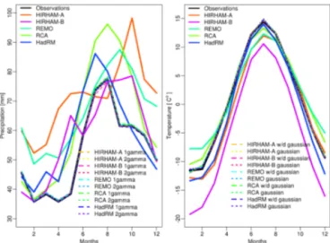
A distinct seasonal cycle can be seen in both temperature and precipitation in Finland (Fig. 4). Annual mean temperature varies from above 5◦C in southern Finland to below−2◦C in northern Finland with maximum monthly mean temperatures in July (ca. 15◦C) and minimum in January–February (ca. −12◦C). The primary peak in seasonal precipitation
accu-mulation occurs in summer (ca. 220 mm season−1) and
sec-ondary in autumn (ca. 180 mm season−1), spring being the
driest season (ca. 110 mm season−1). In this study we define
Figure 4.Monthly mean precipitation accumulation (left) and tem-perature (right) in observations and RCMs in Finland during the control period 1961–2000. Observations (black) and uncorrected RCMs (colours) in solid lines, adjusted RCMs in dashed and dotted lines. Monthly mean precipitation adjusted with single gamma (1-gamma) are presented as dashed lines, and with double gamma (2-gamma) as dotted lines (left panel). Monthly mean temperatures ad-justed with wet–dry state separation (w–d Gaussian) are presented as dashed lines and without wet–dry separation (Gaussian) as dot-ted lines (right panel). All adjusdot-ted values follow closely the ob-servations and no big differences can be seen between the two bias correction procedures.
torrential precipitation to be daily precipitation accumulation exceeding 20 mm day−1which is the official threshold value used in FMI.
3.1 RCM temperature and precipitation in control period
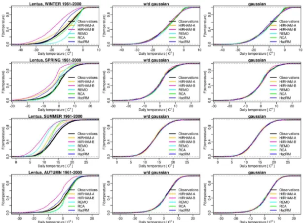
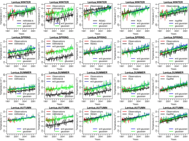
The five RCMs used in this study are able to capture the an-nual cycle of temperature in the control period quite well, but monthly temperatures are commonly underestimated throughout the year except in winter by RCA and REMO and in autumn by HIRHAM-A (Fig. 4). The CDFs show that all RCMs cumulate too much below 0◦C temperatures and too
little above 0◦C temperatures especially in spring, although
also in winter and autumn (Fig. 5).
Figure 5.Cumulative distribution functions for daily temperature in Lentua catchment during the control period 1961–2000. Observations and uncorrected RCM data in left column, daily RCM temperatures adjusted with wet–dry state separation (w–d Gaussian) are presented in middle column and without wet–dry separation (Gaussian) in right column. Winter is shown in first row, spring in second row, summer in third row and autumn in bottom row. All the adjusted values closely follow the observed distribution and no big differences can be seen between the two bias correction procedures.
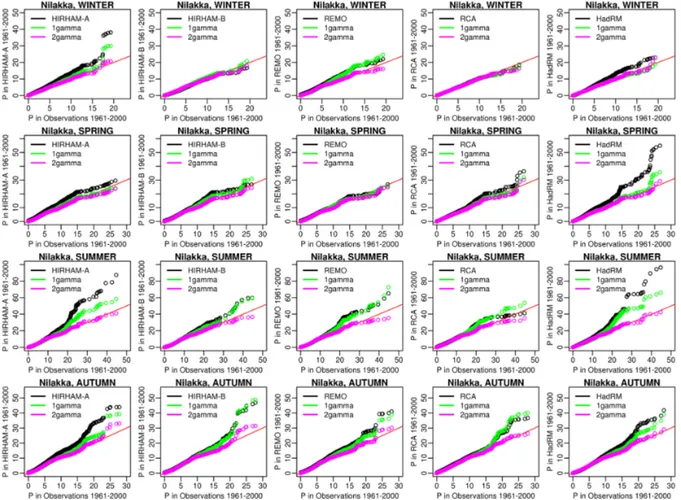
Figure 6. Distribution of daily precipitation amounts during the control period 1961–2000 spring in Nilakka catchment in obser-vations and uncorrected RCM data (top panel), single Gamma-adjusted RCM data (middle panel) and double Gamma-Gamma-adjusted RCM data (bottom panel). Notice the uneven precipitation divi-sion and different scaling for precipitation amounts greater than 20 mm day−1.
too high percentage of light precipitation (≤1 mm day−1; Fig. 6). Occurrence of torrential (>20 mm day−1) precipita-tion events is overestimated in RCMs in every catchment and season.
After applying the DBS method, biases in seasonally calculated daily mean temperatures in uncorrected RCM data are significantly reduced (Figs. 4, 5), from −8.7–5.3 to −0.2–0.5◦C. Also the standard deviation of the DBS-adjusted values is closer to observed values than that of un-corrected RCM data (not shown). DBS scaling preserves the RCM temperature variability in CDFs. The strong temper-ature increase around 0◦C found in the uncorrected RCM
data is reduced after DBS scaling but can still be found from the CDFs (Fig. 5), although shifted towards observed values and higher temperatures. Daily temperatures adjusted with wet–dry separation produce more frequently higher winter maxima (>5◦C) and lower minima (<−30◦C) than
Table 2.Deviation between observed and RCM accumulated seasonal precipitation during control period 1961–2000 in uncorrected and DBS-adjusted (single gamma is 1 gamma, double gamma is 2 gamma) precipitation in percent. Values are shown for Loimijoki in southern Finland and Ounasjoki in northern Finland to demonstrate the spatial variation.
Uncorrected 1 Gamma 2 Gamma Uncorrected 1 Gamma 2 Gamma Loimijoki Ounasjoki
W
inter
HIRHAM-A 53.04 0.23 −0.05 45.27 −0.53 −0.55 REMO 12.22 0.52 0.19 34.55 0.04 −0.26 RCA 5.42 0.04 −0.18 5.93 −0.59 −0.57 HadRM −0.62 −0.76 −0.46 12.37 −1.49 −0.88 HIRHAM-B 2.11 −0.69 −0.65 −3.85 −0.86 −0.53
Spring
HIRHAM-A 77.04 0.73 0.39 80.50 1.58 0.74 REMO 29.71 1.04 0.59 54.51 1.58 0.73 RCA 30.91 0.47 0.26 23.75 0.44 0.16 HadRM 42.41 0.22 0.15 35.76 −0.55 −0.23 HIRHAM-B 40.80 0.93 0.57 39.34 1.31 0.64
Summer
HIRHAM-A −21.75 −2.72 −1.26 16.81 −1.16 −0.46 REMO 2.90 −0.09 0.03 16.44 0.15 0.09 RCA 27.19 1.29 0.56 17.31 0.51 0.23 HadRM 1.27 −0.15 −0.03 26.88 −0.67 −0.20 HIRHAM-B −20.53 −1.47 −0.63 −1.38 −1.47 −0.60
Autumn
HIRHAM-A 24.27 −0.54 0.01 55.70 0.59 0.49 REMO 6.65 0.35 0.42 41.47 1.08 0.78 RCA 22.94 0.91 0.68 34.23 1.22 0.72 HadRM −10.56 −0.61 −0.12 18.65 −0.53 0.06 HIRHAM-B 17.17 0.87 0.85 21.96 0.26 0.31
observations. Due to the cases where daily winter maxima were excessively too high (e.g.>15◦C in January) in DBS
with wet–dry state separated data, we decided to use the DBS method without separation in further analysis of hydrological simulations.
Both single and double gamma DBS approaches for pre-cipitation are able to reduce biases in seasonal prepre-cipitation accumulation from −22–81 to −3.0–1.7 % (Figs. 4, 6; Ta-ble 2) in all catchments. Distribution of drizzle and torrential precipitation is shifted towards observations and the number of dry days is forced to match observed values (Fig. 6).
There are no considerable differences in monthly mean ac-cumulated precipitation between single and double gamma DBS. The largest differences are found in the treatment of heavy (>95th percentile of CDF) precipitation (Figs. 6, 8). Considering daily mean precipitation amounts in the heavy precipitation distribution, DBS with double gamma overes-timates daily mean heavy precipitation amounts in July by 0.2–6.5 % and DBS with single gamma by 12.0–21.7 % in Loimijoki and in Ounasjoki by−0.3–1.3 and by 3.4–14.8 %, respectively, compared to observed values. Due to a longer tail in the single gamma distribution in the heavy precipita-tion end of the distribuprecipita-tion, the high values are in many cases larger and more frequent with single gamma than with double gamma DBS. In some cases the single gamma DBS approach even increases heavy precipitation values compared to
ob-served values. Nevertheless, single gamma distribution was slightly better than double gamma, e.g., in winter and spring in northern Finland (root mean square error (RMSE) 2.78– 3.10 in single gamma and 3.07–3.10 in double gamma in January in Ounasjoki). Still, in most cases the double gamma distribution produces heavy precipitation values closer to ob-served values than single gamma.
3.2 RCM temperature and precipitation in the future
Finland is expected to experience a warmer and wetter cli-mate towards the end of this century. Future changes in sea-sonal precipitation and mean temperature in Loimijoki catch-ment are shown in Table 3. After DBS adjustcatch-ment, seasonal temperature increase varies from 1.4 to 5.1◦C in Loimijoki
and from 1.3 to 6.6◦C in Ounasjoki in the latter part of this
dou-Figure 7.Comparison between uncorrected (black) and DBS-adjusted (pink without wet–dry state separation and green with wet–dry state separation) daily temperatures during control period 1961–2000 in Lentua. Red line corresponds to the observations.
ble gamma DBS-adjusted values. Future changes in seasonal precipitation sums vary more than temperature depending on RCM as well as season and area of investigation, and can even decrease by the end of this century. After DBS adjust-ment the change in seasonal precipitation sums varies from 1.7–39 % in Nilakka to−7.5–37.7 % in Loimijoki by the end of this century, being largest in winter.
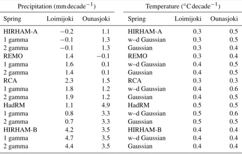
The DBS method preserves the temperature trend of the uncorrected RCM data during 1961–2100 relatively well (Table 4; Fig. 9). The projected temperature trends in un-corrected RCM data vary between 0.3 and 0.5◦C decade−1
in the used scenarios. The differences between uncorrected RCM and DBS-adjusted seasonal trends are mainly less than ±0.1◦C decade−1(Table 4). The largest differences between
temperature trends in uncorrected and DBS-adjusted data can be seen in the scenarios of REMO and RCA, which produce more than 0.1◦C decade−1larger temperature rise after DBS (Fig. 9). This is probably due to a too narrow temperature dis-tribution (low standard deviation) in the control period com-pared to observed values (not shown). In the scenario period the standard deviation decreases even further, with increasing daily temperatures, causing more pronounced warming after DBS adjustment. Other climate models in this study do not
produce any prominent decrease in standard deviation during the scenario period and thus the trends are better preserved.
Also trends in precipitation are preserved sufficiently well among RCMs after DBS adjustment and no distinct differ-ences between RCMs or the two DBS methods can be found. In Loimijoki and Ounasjoki catchments most of the un-corrected scenarios show positive precipitation trends from 1.1 to 4.2 mm decade−1 (Table 4). Only HIRHAM-A in
Loimijoki and REMO in Ounasjoki do not show signifi-cant trends. The differences between RCM and adjusted sea-sonal trends are mainly from −0.6 to +0.3 mm decade−1
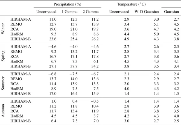
Table 3.Changes in uncorrected and DBS-adjusted RCM seasonal precipitation sums in % and daily mean temperatures as◦C between
control (1961–2000) and scenario periods (2051–2090). Values are shown for winter and spring in Loimijoki catchment in southern Finland.
Precipitation (%) Temperature (◦C)
Uncorrected 1 Gamma 2 Gamma Uncorrected W–D Gaussian Gaussian
W
inter
HIRHAM-A 11.0 12.3 11.2 2.9 3.0 2.7
REMO 12.7 15.7 13.9 3.4 5.1 4.5
RCA 19.0 21.0 19.7 3.6 4.7 4.2
HadRM 9.3 8.9 8.6 4.4 5.0 4.5
HIRHAM-B 23.6 25.4 26.2 4.9 4.3 3.8
Spring
HIRHAM-A −4.6 −4.0 −4.6 2.7 2.6 2.5
REMO 9.2 13.2 11.7 2.8 3.4 3.3
RCA 16.7 17.1 17.8 2.7 3.8 3.6
HadRM 6.7 7.3 6.1 4.5 4.3 4.1
HIRHAM-B 27.1 37.7 34.2 3.8 3.5 3.4
Summer
HIRHAM-A −6.8 −7.5 −6.7 2.1 2.4 2.4
REMO 13.7 14.0 13.6 2.3 2.9 2.7
RCA 11.4 13.9 13.3 2.0 3.3 3.2
HadRM 8.9 7.5 7.5 4.0 4.3 4.2
HIRHAM-B 17.0 16.4 15.9 1.4 1.4 1.5
Autumn
HIRHAM-A 1.0 0.4 −0.5 1.4 1.4 1.4
REMO 11.2 11.8 10.4 2.8 3.9 3.6
RCA 11.7 13.4 11.9 2.8 3.8 3.5
HadRM 4.5 4.5 3.7 4.2 4.3 4.0
HIRHAM-B 6.4 7.3 7.0 3.0 2.7 2.5
3.3 Impact of bias correction on simulated hydrology
The discharges simulated with uncorrected RCM values (Fig. 11) show large differences compared to the observed discharges and discharges simulated with observed meteo-rological input values in the control period (hereinafter re-ferred to as “control simulation”). The differences in sim-ulated mean discharges in the control simulation and using RCM data with and without DBS adjustment for Loimijoki and Ounasjoki test sites are shown in Table 3. In the four test sites the annual mean discharges simulated with uncor-rected RCM inputs were 16–104 % larger than annual mean discharges of the control simulation. The higher annual mean discharges are mainly caused by overestimation of precipita-tion in RCMs.
The seasonal differences are more pronouncedly affected by temperature biases in the RCM data. The HadRM and HIRHAM-B have negative temperature biases during win-ter, which cause smaller winter discharges in southern and central Finland. The negative temperature biases in spring (HIRHAM-B) cause a delay in the spring flood peak (Fig. 11). This delay causes negative biases to mean spring discharges in northern Finland even though the snowmelt floods are larger due to greater snow accumulation caused by positive precipitation and negative temperature biases. Summer mean discharges become larger with all uncorrected
RCM outputs due to positive precipitation biases and larger recession flows caused by greater and delayed spring floods. Using single gamma or double gamma precipitation cor-rections and temperature corcor-rections without wet–dry sepa-ration, the biases in simulated mean discharges can be ef-fectively reduced (Table 5). The differences in annual mean discharges decreased to less than 12 % in all test sites with DBS-adjusted RCM outputs. The difference is at the same level as the difference between control simulation discharges and observed discharges (less than 13 %), which indicates that biases in annual mean discharges are partly explained by the model sensitivity on input variables and partly by the residual biases in corrected RCM outputs.
Figure 8.Comparison between uncorrected (black) and DBS-adjusted daily precipitation (single gamma in green and double gamma in pink) during control period 1961–2000 in Nilakka. Red line corresponds to the observations.
Even though the DBS method corrects the mean tempera-tures efficiently close to observations, the remaining biases in winter temperature extremes, which in control period are slightly above zero, cause remarkable biases in winter dis-charges and snow accumulation in the hydrological simula-tion. However, the seasonal variations in mean discharges af-ter the DBS adjustment are remarkably closer to variations of control simulation (Fig. 11), highlighting the fact that the bias correction is required for RCM data used in studies of climate change effects on hydrology.
In addition to biases in RCM temperature and precipitation data, the biases in wind speed (WS) and specific humidity (SH) also affect the WSFS discharge simulations for catch-ments with high lake percentages. Biases in WS and SH of RCMs affect the lake evaporation in the hydrological model and typically cause a 5–45 % bias in the annual lake evapora-tion sums. In most of the study catchments the bias is largest in the RCA scenario giving 25–35 % negative bias caused by positive bias of SH and negative bias of WS. The bias in lake evaporation can be effectively decreased to 0–13 % by the simple mean bias correction method (Fig. 12).
The uncorrected WS and SH of RCMs cause a 0–11 % bias in annual mean discharges, and a 0–20 % bias in
au-tumn mean discharges in the outlet of Nilakka, which has the highest lake percentage of the study catchments (18 %). In the catchments of Loimijoki and Lentua the biases in mean discharges (0–2 and 0–4 %) and autumn discharges (0–7 and 0–8 %) are smaller, and in the most northern located catch-ment of Ounasjoki the bias is insignificant.
Figure 9.Seasonal trends in observed (red, 1961–2000) and RCM simulated daily temperatures in Lentua basin during 1961–2090. Uncor-rected RCM daily temperatures in black, temperatures adjusted with wet–dry separation in blue and without wet–dry separation in green.
and none of the different DBS approaches are found to be su-perior with respect to mean discharges. Thus, the selection of the best methods is based on the performance of the correc-tion method in decreasing the extreme temperature and pre-cipitation biases, in which the temperature correction without wet–dry separation and double gamma for precipitation work significantly better.
Because of the biases in uncorrected RCM data, the mean discharge peaks caused by snowmelt (Fig. 11) are signifi-cantly larger than the control simulation discharge peaks, and the seasonal variation of discharges is also altered. Without effective bias correction the results of climate change im-pact studies could easily lead to false conclusions. The effect of DBS adjustment on changes in seasonal mean discharges is more pronounced than on annual discharges, because the temperature biases of uncorrected data have significant influ-ence on seasonal discharges. The changes in mean winter and spring discharges may be 2 or even 3 times larger than with-out temperature correction (Fig. 13). If only temperature bias
is corrected, the relative changes are close to the changes in temperature and precipitation corrected data, but the absolute changes are much larger due to wet bias in RCM data.
Table 4.Trends in seasonal precipitation sum (mm decade−1) and temperature (◦C decade−1) in uncorrected and DBS-adjusted RCM simu-lations. Values are shown for spring in Loimijoki and Ounasjoki to demonstrate the spatial variation.
Precipitation (mm decade−1) Temperature (◦C decade−1)
Spring Loimijoki Ounasjoki Spring Loimijoki Ounasjoki HIRHAM-A −0.2 1.1 HIRHAM-A 0.3 0.5 1 gamma −0.1 1.3 w–d Gaussian 0.3 0.5 2 gamma −0.1 1.3 Gaussian 0.3 0.4 REMO 1.4 −0.1 REMO 0.3 0.4 1 gamma 1.6 0.1 w–d Gaussian 0.4 0.5 2 gamma 1.4 0.1 Gaussian 0.4 0.5
RCA 2.3 1.5 RCA 0.3 0.3
1 gamma 1.8 1.2 w–d Gaussian 0.4 0.6 2 gamma 1.9 1.2 Gaussian 0.4 0.5 HadRM 1.1 4.9 HadRM 0.5 0.5 1 gamma 0.8 3.3 w–d Gaussian 0.5 0.6 2 gamma 0.7 3.3 Gaussian 0.5 0.5 HIRHAM-B 4.2 3.5 HIRHAM-B 0.4 0.4 1 gamma 4.7 3.5 w–d Gaussian 0.4 0.4 2 gamma 4.4 3.5 Gaussian 0.4 0.4
The ability of the DBS method to preserve the precipita-tion and temperature trends (Figs. 9, 10) in most cases leads to similar changes in simulated annual mean discharges with uncorrected and DBS-adjusted RCM data (Fig. 13 and Ta-ble 6). In the HadRM-scenario, the DBS-adjusted data pro-duce a lower increase than the uncorrected scenario in north-ern Finland, due to a smaller increase in precipitation trends after DBS adjustment. In northern Finland the differences between the results from simulations with uncorrected and DBS-adjusted data are clearest in spring, when the absolute biases in mean discharges in the control period are highest. The uncorrected HIRHAM-A and HIRHAM-B produce neg-ative bias in mean spring discharges in the control period due to delayed spring floods. Thus, without bias corrections these scenarios produce too high increases in mean spring discharges.
3.4 Future scenarios for discharges
The results show that climate change will have a signifi-cant impacts on seasonality of discharges in Finland due to increasing precipitation and shorter wintertime, which in-fluence snow accumulation and increase evapotranspiration (Fig. 14). The springtime snowmelt floods will occur earlier and the average wintertime discharges will increase because the temperature will rise more often above zero in winter in-creasing rainfall and causing occasional snowmelt. The sum-mer discharges will decrease due to earlier snowmelt and increased evapotranspiration, while the changes in autumn depend on the climate scenario, location and hydrological characteristics such as lake percentage of the study catch-ments. The DBS method influences significantly the pro-jected changes of the seasonal discharges and in some cases
even the annual discharges of the scenarios with large tem-perature biases.
The changes in annual mean discharges between the con-trol and 2051–2090 periods in all study catchments are be-tween−15 and 26 % (Table 6). For the period 2051–2090 HIRHAM-B produces the largest increases in annual mean discharges in all study catchments due to the largest increases in annual mean precipitation. Most of the scenarios show an increase in annual discharges, but especially for southern and central Finland some scenarios project decrease because the longer and warmer summers will cause a larger increase in evapotranspiration than the projected increase in precipita-tion.
In the study catchments all DBS-adjusted scenarios pre-dict on average 2–4 weeks earlier snowmelt discharge peaks in spring for the 2051–2090 period compared to the control period 1961–2000. Figure 14 shows the results for three sce-narios producing the largest variation of changes in mean dis-charges out of five scenarios used in this study. Because the snowmelt discharge peaks occur earlier, the recession flows in summer season decrease. The summer discharges decrease 20–50 % in all scenarios except in Nilakka and Loimijoki in the HIRHAM-B-scenario, which predicts a greater increase in precipitation than the other scenarios. The decrease in mean summer discharges is caused by the increase of the an-nual evapotranspiration by 10–40 % and lake evaporation by 10–80 %.
Figure 10.Seasonal trends in observed (red, 1961–2000) and RCM simulated seasonal precipitation accumulation in Ounasjoki catchment during 1961–2090. Uncorrected RCM precipitation in black, precipitation adjusted with single gamma in blue and with double gamma in green.
winter discharges increase 10–70 %, depending on the used scenario.
The results show an increase in autumn mean discharges in northern Finland, where the autumn runoff peaks – typi-cal in southern Finland at present – become more frequent. In the catchments with large lake percentages in southern and central Finland, the autumn mean discharges decrease in all scenarios due to an increase in evapotranspiration and larger soil moisture deficit in the beginning of autumn. In the southern catchments with low lake percentages, the change in mean autumn discharges depends on the scenario. Differ-ent autumn precipitation changes between the scenarios are the main reason for different changes in autumn discharges, but also the soil moisture content after summer has an influ-ence and varies depending on temperature and precipitation changes during summer.
The relative changes in mean discharges, MHQ and MNQ together with changes in mean maximum snow water
equiv-alent (SWE), mean maximum soil moisture deficit (SMD), mean evapotranspiration (ET) and mean runoff (R) in four test sites are shown in Fig. 15. The changes in annual high flows are mostly negative, due to decreased maximum SWE and consequently decreasing spring snowmelt floods. Only in the HIRHAM-B scenario the MHQ increase or remains the same in most test sites due to large increase in precip-itation. The annual low flows decrease in southern Finland due to increased ET and maximum SMD, due to decrease in low flows in summer season. In northern Finland the annual MNQ increase, because the annual low flows normally occur in winter in the control period.
4 Discussion
dif-Figure 11.Hydrographs of simulated daily mean discharges in 1961–2000 with uncorrected RCM outputs (dashed lines) and corrected temperatures (T Gaussian) and precipitation (P double gamma) (solid lines) compared to control simulation discharges (blue line).
Figure 12.Model mean lake evaporation sums and simulated daily mean discharges of Lake Nilakka and Lake Lentua with RCA uncorrected WS and SH (T is Gaussian,P is 2gamma) in red, with corrected WS and SH (T is Gaussian,P is double gamma) in green and control simulation in blue.
fer significantly from observations. Bias correction is nec-essary since RCM biases not only affect the absolute dis-charges, but also can influence the relative changes (Leander et al., 2008). As shown in the previous section the projected seasonal changes of the mean discharges in Finland are espe-cially sensitive to RCM biases, because both the temperature and precipitation biases significantly influence the mean dis-charges.
Several studies comparing different bias correction meth-ods have concluded that generally it is not possible to
Table 5.Deviation of simulated annual and seasonal mean discharges (MQ) between observed, uncorrected and DBS-adjusted temperature (Gaussian) and precipitation (1 or 2 gamma) as input for hydrological simulations during control period 1961–2000 in %. Values are shown for Loimijoki in southern Finland and Ounasjoki in northern Finland to demonstrate the spatial variation.
Uncorrected 1 Gamma 2 Gamma Uncorrected 1 Gamma 2 Gamma Loimijoki Ounasjoki
Y
ear
HIRHAM-A 85.7 9.5 10.1 104.2 3.3 3.2 REMO 58.0 12.3 11.8 78.6 5.7 5.1 RCA 89.0 12.7 11.5 48.5 4.9 4.4 HadRM 35.3 9.4 9.8 48.9 1.9 2.8 HIRHAM-B 63.3 10.0 9.8 56.6 2.9 3.1
W
inter
HIRHAM-A 86.7 22.9 22.1 85.7 12.5 12.6 REMO 16.4 −22.4 −21.7 73.8 −7.9 −8.3 RCA 33.5 −12.1 −12.3 67.5 3.8 3.2 HadRM −43.3 60.3 61.8 18.8 34.2 35.5 HIRHAM-B −46.1 79.1 79.0 19.1 46.7 46.7
Spring
HIRHAM-A 92.9 10.0 10.1 −20.8 −0.6 −0.8 REMO 57.0 27.6 26.8 39.0 1.2 0.9 RCA 54.6 23.8 23.4 43.9 8.7 8.5 HadRM 67.7 −9.5 −9.5 12.2 −2.5 −2.0 HIRHAM-B 64.1 −16.6 −16.5 −76.4 3.4 3.6
Summer
HIRHAM-A 142.8 7.2 8.2 231.8 3.0 2.8 REMO 161.4 38.6 35.2 108.3 20.1 19.0 RCA 238.0 28.6 22.7 21.6 0.7 0.2 HadRM 140.5 4.9 3.7 97.0 −0.7 0.3 HIRHAM-B 308.2 −4.5 −5.1 220.7 −14.0 −13.8
Autumn
HIRHAM-A 44.3 −2.7 −0.2 117.9 6.7 6.8 REMO 51.4 1.1 1.2 99.7 −4.1 −4.7 RCA 143.0 5.7 3.8 92.2 5.96.0 4.7 HadRM −2.3 7.3 8.1 46.6 0.0 1.1 HIRHAM-B 57.7 11.5 11.0 32.6 10.8 11.2
the need to extrapolate data in both ends of the QM function (e.g. Veijalainen et al., 2012; Räisänen and Räty, 2013). With DBS used in this study no extrapolation is needed because continuous distribution functions are used to adjust tempera-ture and precipitation, and DBS is thus considered to be more sophisticated method.
Although bias correction methods usually improve the RCM simulations substantially, other uncertainties still re-main, especially for future simulations. Biases in RCMs, changing trends due to different correction procedures, and non-stationarity of climate conditions have been investigated, e.g., by Teutschbein and Seibert (2013), Maraun (2012) and Maraun (2013). One disadvantage of bias correction is that the physical cause of precipitation and temperature bias is not taken into account. For instance a few degrees bias in temperature in winter affects the form of precipitation and snowmelt, which have significant impact on snow accumu-lation in hydrological models. A recent study by Räisänen et al. (2014) found that during the snowmelt period in the ECHAM5 model, the air temperature rarely rises above zero as long as there is snow on the ground, leading to too low
temperatures during the snowmelt period. This study shows that even after the DBS adjustment the biases in the near-zero temperatures remain. Especially with the RCA and REMO, which were driven by boundary conditions from ECHAM5, these biases influence the magnitude of winter and spring runoff and floods in the hydrological model simulations. Ma-raun (2013) stated that bias correction can even deteriorate future simulations and increase the future bias especially in areas where biased responses of surface albedo, soil mois-ture or cloud cover affected RCM simulations. According to Maraun (2013), biases are however relatively stable and bias correction on average considerably improves climate scenar-ios.
per-Table 6.Relative changes (%) in simulated annual and seasonal mean discharges (MQ) in Loimijoki and Ounasjoki between control period 1961–2000 and future period 2051–2090 using uncorrected and DBS-adjusted temperature (Gaussian) and precipitation (1 or 2 gamma).
Uncorrected 1 Gamma 2 Gamma Uncorrected 1 Gamma 2 Gamma Loimijoki Ounasjoki
Y
ear
HIRHAM-A −3.8 −5.9 −8.1 9.1 9.1 9.0 REMO 7.4 10.5 6.8 −0.3 −5.5 −5.3
RCA 10.1 9.8 8.5 8.6 3.4 3.4
HadRM −6.8 −6.8 −7.6 15.3 5.0 6.1 HIRHAM-B 16.0 25.6 24.7 17.7 18.7 18.0
W
inter
HIRHAM-A 69.8 65.2 63.1 71.1 90.3 89.8 REMO 104.2 151.5 141.1 68.6 40.9 40.6 RCA 107.6 143.2 140.0 73.8 76.4 76.6 HadRM 204.5 37.7 36.5 76.1 128.9 131.8 HIRHAM-B 148.0 50.7 51.2 44.9 74.9 68.4
Spring
HIRHAM-A −25.6 −32.2 −33.3 134.3 26.0 26.0 REMO −18.6 −21.9 −23.4 24.2 20.2 19.8 RCA −21.9 −23.8 −23.7 −1.1 11.5 12.0 HadRM −31.3 −29.6 −29.4 72.3 4.2 5.2 HIRHAM-B 21.2 17.5 14.7 206.3 16.5 18.1
Summer
HIRHAM-A −31.7 −31.3 −32.9 −39.1 −39.7 −39.6 REMO −17.0 −27.7 −31.6 −43.9 −49.8 −49.2 RCA −5.9 −34.4 −35.8 −20.3 −41.3 −41.2 HadRM −25.4 −23.3 −25.4 −38.5 −49.7 −49.3 HIRHAM-B −34.5 2.2 1.3 −9.1 −17.7 −17.7
Autumn
HIRHAM-A −10.6 −15.2 −19.5 28.3 21.9 21.5 REMO 13.0 18.0 11.5 18.8 19.1 19.6 RCA 12.5 12.2 8.2 26.2 27.5 26.8 HadRM −13.0 −22.1 −23.7 37.5 23.0 24.4 HIRHAM-B 23.1 9.5 9.1 55.6 36.1 34.2
formance of six different bias correction procedures under systematically varying climate conditions. They found DBS performed the best out of the studied bias correction methods under changing conditions and questioned the use of sim-ple bias correction methods such as delta change and lin-ear scaling. Without the possibility to validate future sce-narios against observed values the best policy, according to Teutschbein and Seibert (2012), is to use an ensemble of RCMs with the best available bias correction method.
The current study shows that the effect of DBS adjustment on temperature and precipitation trends is generally small. But with a large bias in standard deviation of the uncorrected temperature data, the DBS may cause a significant change in temperature trends, increasing the uncertainty for the climate change projections. Also since the precipitation and temper-ature corrections are not interdependent, in some cases the bias in the snow accumulation remains considerably large, which leaves biases in spring discharges during the control period and certainly affects the relative changes in the future. Räisänen and Räty (2013) and Räty et al. (2014) concluded that since no single BC method outperforms others in all cir-cumstances, the use of a few different but well-performing
correction methods will give a more realistic range of un-certainty. In the hydrological studies the assessment of the performance should be based on the remaining biases in dis-charges during the control period to avoid unnecessary large uncertainty range and false conclusions about the impacts of climate change.
Figure 13.The minimum, maximum, 1st and 3rd quartile and me-dian deviations of the simulated mean discharges with RCM data compared to control simulations (above) and climate change im-pacts (below) in four test sites using all five scenarios without cor-rections (unc), only with temperature correction (T w–d is wet–dry separation andT cor is without separation) or precipitation correc-tions (1-G is single gamma and 2-G is double gamma) and with both temperature and precipitation corrections.
20–30 % of days in autumn and winter in Finland are con-sidered to be dry. For precipitation distribution the removal of drizzle days is important, but for temperature it is ques-tionable whether the simulated temperature for drizzle days represents the temperature for dry days. Separation of days according to wet–dry state reduces the number of days avail-able for the temperature distribution on wet–dry days, which can cause biases in CDFs especially in the lower and upper tails of the distribution. Due to the tendency of wet–dry sep-aration to produce too low minima and too high maxima the DBS approach without wet–dry separation produces better fit with observed values in most cases in Finland.
The DBS method with wet–dry separation roughly takes into account the correlation between temperature and precip-itation, but precipitation is still adjusted without knowledge of temperature. It would not be rational to divide precipi-tation events according to near surface temperature since it does not determine the precipitation phase, but instead tem-perature at 850 hPa could be used. Also separation accord-ing to weather types could take stratiform and torrential pre-cipitation events better into account. The problem with these methods is the lack of comprehensive observational data and thus some reanalysis or other climate models should be used as observational data in the adjustment.
Two distributions, single and double gamma, were used for precipitation corrections. The double gamma distribu-tion is expected to produce better fit with observed pre-cipitation, compared to single gamma, due to better
perfor-mance with torrential precipitation. However, depending on season and area of investigation single gamma distribution fitted observed values and RCM simulations better than dou-ble gamma distribution (e.g. RMSE 4.8–5.8 in single gamma and 5.4–5.6 in double gamma in Loimijoki and 2.8–3.0 in single gamma and 3.1 in double gamma in Ounasjoki in Jan-uary). In these cases the area of investigation had not expe-rienced many torrential precipitation events and a large part of the distribution consisted of drizzle days. Although dou-ble gamma usually reproduces torrential precipitation events better than single gamma, the cut-off value of 95 % does not always produce the best results. At least for colder regions like Finland where torrential precipitation events are rela-tively rare, the cut-off value could be even higher (e.g. 98 %) to get better gamma fit also for the torrential values. After applying the 95 % cut-off value, the torrential 5 % means roughly precipitation values higher than 10 mm day−1, al-though by definition 20 mm day−1 is the threshold for tor-rential precipitation in Finland. In addition, the highest 5 % of precipitation distribution does not in most cases produce real gamma function and thus the gamma fit might not be valid. One problem with double gamma distribution occurred near (below and above) the cut-off value for heavy precipi-tation because it caused discontinuity in the distribution and thus cumulated too much precipitation around this point. In Finland this means an increase in near 10 mm day−1
precip-itation amounts compared to observed values. Considering accumulated monthly mean precipitation amounts below and above the 95 % cut-off value, we observed that in most cases DBS with double gamma accumulated more precipitation be-low the 95 % cut-off value and less above the 95 % cut-off value than single gamma (e.g. from −1.3 to 7.8 % below the 95 % cut-off value and from−26.2 to 0.7 % above the 95 % cut-off value in March in Loimijoki). Nevertheless, the monthly total accumulated precipitation is better represented by DBS with double gamma distribution when compared to observed values. For example DBS with double gamma gives 0.3–0.8 % higher monthly mean precipitation accumulation than observations in March in Loimijoki and DBS with sin-gle gamma 0.3–1.3 %.
Precipitation varies considerably on spatial and temporal scales and thus to use either single or double gamma distribu-tion alone is a somewhat rigid procedure. The importance of the torrential precipitation is more pronounced in the impact studies of flash floods and floods in small river catchments, which respond quickly to extreme precipitation. In the larger watersheds, the high discharges usually correlate better with 5–15-day extreme precipitation sums than torrential values due to the delay caused by soil moisture deficit, river trans-port, lake storage and wetlands inside the catchment. Thus, the tendency of double gamma correction to increase the near 10 mm day−1precipitation may deteriorate the DBS ability
de-Figure 14.Hydrographs of simulated daily mean discharges with DBS-adjusted temperatures (T Gaussian without separation) and precipi-tation (P double gamma) of RCMs in 1961–2000 (solid lines) and in 2051–2090 (dashed lines) compared to control simulation discharges (blue line).
Figure 15.The minimum, maximum, 1st and 3rd quartile and me-dian changes by 2051–2090 period in mean discharges (MQ), mean high discharges (MHQ), mean low discharges (MNQ), mean maxi-mum snow water equivalent (maxSWE), mean maximaxi-mum soil mois-ture deficit (maxSMD), mean annual evapotranspiration (ET) and runoff (R) in four test catchments and five scenarios with Gaussian and double gamma-adjusted RCM data.
veloped, but problems would occur when either observed or RCM simulated precipitation would not produce the same selection of gamma distribution.
Previously the most commonly used method to esti-mate cliesti-mate change impacts on hydrology was the delta change method (e.g. Andréasson et al., 2004; Steele-Dunne et al., 2008; Veijalainen et al., 2010). Often a very simple ver-sion of this method, where only the monthly mean changes of temperature and precipitation from climate model simu-lations were used to modify the observed temperature and precipitation records, was used (Hay et al., 2000). Compared to delta change methods, the BC methods better preserve the variability in temperature and precipitation produced by the RCMs (Lenderink et al., 2007; Graham et al., 2007; Beldring
et al., 2008; Yang et al., 2010). Veijalainen (2012) showed that with delta change and with the QM method, the changes in discharges for four catchments in Finland were similar for annual means. However, larger differences were found in flood estimates and in seasonal values. Especially dur-ing sprdur-ing in northern Finland, the delta change method pro-duced earlier snowmelt than the bias corrected RCM data. The changes in annual and seasonal discharges, as well as in timing of the spring discharge peaks, with DBS-adjusted RCM data of this study are in good agreement with results of the QM method used by Veijalainen et al. (2012). The result supports the idea to use both methods in future studies to bet-ter cover the uncertainty range caused by bias correction. On the other hand the extrapolation of the data in the QM method may increase the uncertainty of the climate projections.
ver-sions of these sub-models would be required for the proper estimation of the hydrological model and overall estimation of the uncertainties.
5 Summary and conclusions
The use of bias corrected RCM data as input to impact mod-els is becoming a common practice. The choice of bias cor-rection method significantly affects estimation of climate change impacts on hydrology. The DBS algorithm has been shown to perform well under changing conditions and out-perform other methods in many cases (Teutschbein and Seib-ert, 2012; Räty et al., 2014) and was therefore selected for this study. Two different DBS methods for temperature (with and without dry/wet day separation) and two for precipita-tion (single and double gamma distribuprecipita-tion) were compared. This paper focuses on mean values of temperature, precipi-tation and discharges simulated with the hydrological model of WSFS in four catchments. The DBS adjustment signifi-cantly improves RCM data and simulated discharges com-pared to observations, but the magnitude of the biases of the uncorrected RCM data still influence the success of the DBS method.
Both gamma distributions used in the DBS method for precipitation provide reasonable results for Finland, where precipitation extremes are moderate in all seasons. Dou-ble gamma distribution reproduces monthly precipitation amounts and torrential values better than single gamma dis-tribution, but the cut-off value in 95th percentile is too low in some cases and it could be better to determine specifically for northern climate conditions. For temperature, the small fraction of dry days during some seasons affects the DBS temperature adjustment with dry/wet separation, and thus for temperature the method without dry/wet separation performs better. With most scenarios the DBS method preserves tem-perature and precipitation trends projected by uncorrected RCMs data sufficiently well. However, in cases when the simulated seasonal cycle of precipitation in RCM is not cor-rect, the DBS adjustment changes the trend more than for cases with a correct seasonal cycle. Also, too narrow standard deviation of uncorrected RCM data compared to observed deviation leads to increased temperature trends after DBS ad-justment with two scenarios. The cold bias found in RCMs during snowmelt can be reduced by DBS method, but the re-maining biases are found to influence the timing of snowmelt and the magnitude of winter and spring discharges in hydro-logical simulations.
The projected changes in annual mean discharges by 2051–2090 are moderate, but seasonal distribution of dis-charges will change significantly. The most notable changes are increasing winter discharges, decreased and earlier spring discharge peaks, and decreasing summer discharges due to longer and warmer summer and increased evapotranspira-tion. The autumn discharges are projected to increase in
northern Finland and decrease in the catchments with high lake percentage in southern Finland. The different RCMs produce a wide range of variability on magnitude of the changes. Contrary to the other scenarios used in this study, the HIRHAM-B scenario produces an increase in summer discharges due to greater precipitation increase. Also the ef-fect of different scenarios on mean autumn discharge in the fast responding southern catchments is scenario dependent.
For relative changes in future discharges, the bias cor-rection mainly affects the seasonal results. The differences between changes in seasonal discharges with corrected and uncorrected RCM data are significant especially in the sce-narios with large temperature biases. The correct seasonal changes are important when any detailed analysis of adap-tation strategies, for example in lake regulation rules or flood risk analysis, are considered. Especially the extremes – floods and droughts – are sensitive to both temperature and precipitation biases and without bias correction even the re-sults of relative changes in floods can be misleading. The im-pact of the bias correction on precipitation extremes and on simulated extreme discharges will be examined in the next phase of this study and published in a separate paper.
Since the choice of the bias correction method influences the results and the best method cannot usually be assessed, an ensemble of bias correction methods to incorporate this uncertainty to the other sources of uncertainty such as choice of emission scenario, climate or hydrological model could be used in the future. However, the evaluation of suffi-ciently well-performing bias correction methods is required to avoid unrealistic results in the climate change impact as-sessments. The remaining biases in temperature and precipi-tation data, independent adjustments for meteorological vari-ables or changing temperature and precipitation trends in some climate scenarios after the DBS adjustment cause addi-tional uncertainty in the hydrological simulations and these should be considered when the results are interpreted.
Acknowledgements. This study was carried out within the project Climate Change and Water Cycle: Effect to Water Resources and their Utilization in Finland (ClimWater) (no. 140930) financed by the Finnish Academy as part of the Research Programme for climate change FICCA. The ENSEMBLES data used in this work were funded by the EU FP6 Integrated Project ENSEMBLES (con-tract number 505539) whose support is gratefully acknowledged. Edited by: E. Morin
References
Andréasson, J., Bergström, S., Carlsson, B., Graham, L., and Lind-ström, G.: Hydrological change – climate change impact simula-tions for Sweden, Ambio, 33, 228–234, 2004.
on two methods for transferring RCM results to meteorological station sites, Tellus A, 60, 439–450, 2008.
Bergström, S.: Development and application of a conceptual runoff model for Scandinavian catchments, SMHI, Norrköping, Report RHO No. 7, 134 pp., 1976.
Castro, M., Gallardo, C., Jylhä, K., and Tuomenvirta, H.: The use of a climate-type classification for assessing climate change effects in Europe from an Ensemble of nine regional climate models, Climatic Change, 81, 329–341, doi:10.1007/s10584-006-9224-1, 2007.
Christensen, J. H., Boberg, F., Christensen, O. B., and Lucas-Picher, P.: On the need for bias correction of regional climate change projections of temperature and precipitation, Geophys. Res. Lett., 35, L20709, doi:10.1029/2008GL035694, 2008. Finnish Environment Institute: available at: www.environment.fi/
waterforecast/, last access: 10 January 2015.
Førland, E. J., Allerup, P., Dahlström, B., Elomaa, E., Jónsson, T., Madsen, H., Perälä, J., Rissanen, P., Vedin, H., and Vejen, F.: Manual for Operational Correction of Nordic Precipitation Data, Norwegian Meteorol. Inst., Oslo, Report 24/96 KLIMA, 66 pp., 1996.
Graham, L. P., Andréasson, J., and Carlsson, B.: Assessing climate change impacts on hydrology from an ensemble of regional cli-mate models, model scales and linking methods – a case study on the Lule River Basin, Climatic Change, 81, 293–307, 2007. Hay, L. E., Wilby, R. L., and Leavesley, G. H.: A comparison of
delta change and downscaled GCM scenarios for three moun-tainous basins in the United States, Journal of American Water Resources Association (JAWRA), 36, 387–397, 2000.
Hewitson, B. C. and Crane, R. G.: Climate downscaling: techniques and application, Clim. Res., 7, 85–95, 1996.
Huttunen, I., Lehtonen, H., Huttunen, M., Piirainen, V., Korppoo, M., Veijalainen, N., Viitasalo, M., and Vehvilänen, B.: Effects of climate change and agricultural adaptation on nutrient loading from Finnish catchments to the Baltic Sea, Sci. Total Environ., 529, 168–181, 2015.
Hyvärinen, V., Solantie, R., Aitamurto, S., and Drebs, A.: Suomen vesitase 1961–1990 valuma-alueittain, Vesi- ja ympäristöhal-litus, Helsinki, Vesi- ja ympäristöhallinnon julkaisuja – sarja A 220, 1995.
Jakkila, J., Vento, T., Rousi, T., and Vehviläinen, B.: SMOS soil moisture data validation in the Aurajoki watershed, Finland, Hy-drol. Res., 45, 684–702, doi:10.2166/nh.2013.234, 2014. Jylhä, K., Tuomenvirta, H., Ruosteenoja, K., Niemi-Hugaerts, H.,
Keisu, K., and Karhu, J. A.: Observed and projected future shifts of climate zones in Europe and their use to visualize climate change information, Weather, Climate and Society, 2, 148–167, doi:10.1175/2010WCAS1010.1, 2009a.
Jylhä, K., Ruosteenoja, K., Räisänen, J., Venäläinen, A., Ruoko-lainen, L., Saku, S., and Seitola, T.: Arvioita Suomen muut-tuvasta ilmastosta sopeutumistutkimuksia varten, ACCLIM-hankkeen raportti 2009, Ilmatieteen laitos, Helsinki, Raportteja 2009:4, 2009b.
Korhonen, J. and Kuusisto, E.: Long-term changes in the discharge regime in Finland, Hydrol. Res., 41, 253–268, 2010.
Leander, R., Buishand, T. A., van den Hurk, B. J. J. M., and de Wit, M. J. M.: Estimation of changes in flood quintiles of the river Meuse from resampling of regional climate model output, J. Hy-drol., 351, 331–343, 2008.
Lenderink, G., Buishand, A., and van Deursen, W.: Estimates of future discharges of the river Rhine using two scenario method-ologies: direct versus delta approach, Hydrol. Earth Syst. Sci., 11, 1145–1159, doi:10.5194/hess-11-1145-2007, 2007. Maraun, D.: Nonstationarities of regional climate model biases in
European seasonal temperature and precipitation sums, Geophys. Res. Lett., 39, L06706, doi:10.1029/2012GL051210, 2012. Maraun, D.: Bias correction, quantile mapping, and
downscal-ing: revisiting the inflation issue, J. Climate, 26, 2137–2143, doi:10.1175/JCLI-D-12-00821.1, 2013.
Nash, J. E. and Sutcliffe, J. V.: River forecasting through conceptual models 1: a discussion of principles, J. Hydrol., 10, 282–290, 1970.
Perälä, J. and Reuna, M.: Lumen vesiarvon alueellinen ja ajallinen vaihtelu Suomessa, Vesi- ja ympäristöhallitus, Helsinki, Vesi- ja Ympäristöhallinnon julkaisuja – sarja A 56, 1990.
Prudhomme, C. and Davies, H.: Assessing uncertainties in climate change impact analyses on the river flow regimes in the UK. Part 2: Future climate, Climatic Change, 93, 197–222, 2009. Räisänen, J. and Räty, O.: Projections of daily mean temperature
variability in the future: cross-validation tests with ENSEM-BLES regional climate simulations, Clim. Dynam., 41, 1553– 1568, doi:10.1007/s00382-012-1515-9, 2013.
Räisänen, P., Luomaranta, A., Järvinen, H., Takala, M., Jylhä, K., Bulygina, O. N., Luojus, K., Riihelä, A., Laaksonen, A., Koski-nen, J., and PulliaiKoski-nen, J.: Evaluation of North Eurasian snow-off dates in the ECHAM5.4 atmospheric general circulation model, Geosci. Model Dev., 7, 3037–3057, doi:10.5194/gmd-7-3037-2014, 2014.
Räty, O., Räisänen, J., and Ylhäisi, J.: Evaluation of delta change and bias correction methods for future daily precipitation: inter-model cross-validation using ENSEMBLES simulations, Clim. Dynam., 42, 2287–2303, 2014.
Rauscher, S. A., Coppola, E., Piani, C., and Giorgi, F.: Reso-lution effects on regional climate model simulations of sea-sonal precipitation over Europe, Clim. Dynam., 35, 685–711, doi:10.1007/s00382-009-0607-7, 2010.
Resio, D. T. and Vincent, C. L.: Estimation of winds over the great lakes, J. Waterw. Port C. Div., 103, 265–283, 1977.
Ruosteenoja, K., Räisänen, J., and Pirinen, P.: Projected changes in thermal seasons and the growing season in Finland, Int. J. Cli-matol., 31, 1473–1487, doi:10.1002/joc.2171, 2011.
Steele-Dunne, S., Lynch, P., McGrath, R., Semmler, T., Wang, S., Hanfin, J., and Nolan, P.: The impacts of climate change on hy-drology in Ireland, J. Hydrol., 356, 28–45, 2008.
Taskinen, A.: Operational correction of daily precipitation measure-ments in Finland, Boreal Environ. Res., in review, 2015. Teutschbein, C. and Seibert, J.: Bias correction of regional climate
model simulations for hydrological climate-change impact stud-ies: review and evaluation of different methods, J. Hydrol., 456– 457, 12–29, 2012.
Teutschbein, C. and Seibert, J.: Is bias correction of re-gional climate model (RCM) simulations possible for non-stationary conditions?, Hydrol. Earth Syst. Sci., 17, 5061–5077, doi:10.5194/hess-17-5061-2013, 2013.
van Pelt, S. C., Kabat, P., ter Maat, H. W., van den Hurk, B. J. J. M., and Weerts, A. H.: Discharge simulations performed with a hy-drological model using bias corrected regional climate model in-put, Hydrol. Earth Syst. Sci., 13, 2387–2397, doi:10.5194/hess-13-2387-2009, 2009.
Vehviläinen, B.: Snow Cover Models in Operational Watershed Forecasting, Publications of Water and Environment Research Institute, 11, National Board of Waters and the Environment, Helsinki, 1992.
Vehviläinen, B. and Huttunen, M.: Climate change and Water Re-sources in Finland, Boreal Environ. Res., 2, 3–18, 1997. Vehviläinen, B., Huttunen, M., and Huttunen, I.: Hydrological
fore-casting and real time monitoring in Finland: the watershed simu-lation and forecasting system (WSFS), in: Innovation, Advances and Implementation of Flood Forecasting Technology, Confer-ence Papers, Tromsø, Norway, 17–19 October 2005.
Veijalainen, N.: Estimation of climate change impacts on hydrol-ogy and floods in Finland, PhD thesis, Aalto University, Espoo, Finland, Doctoral dissertations 55/2012, 211 pp., 2012. Veijalainen, N., Lotsari, E., Alho, P., Vehviläinen, B., and Käyhkö,
J.: National scale assessment of climate change impacts on flood-ing in Finland, J. Hydrol., 391, 333–350, 2010.
Veijalainen, N., Korhonen, J., Vehviläinen, B., and Koivusalo, H.: Modelling and statistical analysis of catchment water balance and discharge in Finland in 1951–2099 using transient climate scenarios, Journal of Water and Climate Change, 3, 55–78, doi:10.2166/wcc.2012.012, 2012.
Wood, A. W., Leung, L. R., Shidhar, V., and Lettenmaier, D. P.: Hy-drological implications of dynamical and statistical approaches to downscale climate model outputs, Climatic Change, 62, 189– 216, 2004.