Geoscientiic
Geoscientiic
Geoscientiic
Geoscientiic
water vapor match
Y. Inai1,*, F. Hasebe2, M. Fujiwara2, M. Shiotani3, N. Nishi4,**, S.-Y. Ogino5, H. V¨omel6, S. Iwasaki7, and T. Shibata8
1Graduate School of Science, Tohoku University, Sendai, Japan
2Faculty of Environmental Earth Science, Hokkaido University, Sapporo, Japan 3Research Institute for Sustainable Humanosphere, Kyoto University, Uji, Japan 4Geophysical Institute, Kyoto University, Kyoto, Japan
5Japan Agency for Marine-Earth Science and Technology, Yokosuka, Japan 6GRUAN Lead Center, Deutscher Wetterdienst, Lindenberg, Germany
7Department of Earth and Ocean Science, National Defense Academy, Yokosuka, Japan 8Graduate School of Environmental Studies, Nagoya University, Nagoya, Japan
*now at: Research Institute for Sustainable Humanosphere, Kyoto University, Uji, Japan **now at: Faculty of Science, Fukuoka University, Fukuoka, Japan
Correspondence to:Y. Inai (yoichi inai@rish.kyoto-u.ac.jp)
Received: 22 November 2012 – Published in Atmos. Chem. Phys. Discuss.: 8 January 2013 Revised: 17 July 2013 – Accepted: 18 July 2013 – Published: 2 September 2013
Abstract.We apply the match technique, whereby the same air mass is observed more than once and such cases are termed a “match”, to study the dehydration process asso-ciated with horizontal advection in the tropical tropopause layer (TTL) over the western Pacific. The matches are ob-tained from profile data taken by the Soundings of Ozone and Water in the Equatorial Region (SOWER) campaign network observations using isentropic trajectories calculated from European Centre for Medium-Range Weather Fore-casts (ECMWF) operational analyses. For the matches iden-tified, extensive screening procedures are performed to ver-ify the representativeness of the air parcel and the validity of the isentropic treatment, and to check for possible water injection by deep convection, consistency between the sonde data and analysis field referring to the ozone conservation. Among the matches that passed the screening tests, we iden-tified some cases corresponding to the first quantitative value of dehydration associated with horizontal advection in the TTL. The statistical features of dehydration for the air parcels advected in the lower TTL are derived from the matches. The threshold of nucleation is estimated to be 146±19 % (1σ) in relative humidity with respect to ice (RHice), while
dehydra-tion seems to continue until RHicereaches about 75±23 %
(1σ) in the altitude region from 350 to 360 K. The efficiency
of dehydration expressed by the relaxation time required for the supersaturated air parcel to approach saturation is em-pirically determined from the matches. A relaxation time of approximately one hour reproduces the second water vapor observation reasonably well, given the first observed water vapor amount and the history of the saturation mixing ratio during advection in the lower TTL.
1 Introduction
Water vapor has strong absorption/emission bands in the in-frared region; accordingly, it has a strong greenhouse effect. In the troposphere and stratosphere, it plays an important role in the radiation balance of the earth (e.g., Forster and Shine, 1999; Solomon et al., 2010), and it influences atmospheric chemistry via its product, the hydroxyl radical (OH) (Stenke and Grewe, 2005), and via polar stratospheric clouds (PSCs) (Saitoh et al., 2006).
understood, whereas the dehydration process in the tropical tropopause region is somewhat unclear despite the fact that it is considered a key factor for understanding stratospheric wa-ter vapor, including its unexplained long-wa-term change (Olt-mans and Hofmann, 1995; Kley et al., 2000; Olt(Olt-mans et al., 2000; Scherer et al., 2008; Fujiwara et al., 2010; Hurst et al., 2011).
In the late 1990s, many studies investigated the transition in meteorological features that occurs within a layer of sev-eral kilometers in height from the troposphere to the strato-sphere in the tropics, and the findings of these studies re-sulted in the concept of the tropical tropopause layer (TTL; e.g., Highwood and Hoskins, 1998; Fueglistaler et al., 2009). In turn, this resulted in an innovative hypothesis, the “cold trap” dehydration hypothesis, regarding the nature of dehy-dration processes in the tropical tropopause region, i.e., air is dehydrated during horizontal advection through the cold trap region in the western tropical Pacific (Holton and Gettelman, 2001). This cold trap dehydration hypothesis, by consider-ing quasi-isentropic motion, indicates that the local tempera-ture minimum can effectively dehydrate the air mass entering the stratosphere. This hypothesis was supported by General Circulation Model (GCM) simulations (Hatsushika and Ya-mazaki, 2003). As a result, this dehydration process is con-sidered to be efficiently driven by equatorially symmetric at-mospheric gyres and by the “cold trap” that forms in the TTL as a response to heating at the lower boundary in the western tropical Pacific (Matsuno-Gill pattern; Matsuno, 1966; Gill, 1980).
Fueglistaler et al. (2005) and Ploeger et al. (2011) esti-mated the water vapor amount on a 400 K potential tem-perature surface corresponding to the top of the TTL by using the Lagrangian relative humidity history along tra-jectories with simplified condensation and a water-removal scheme. European Centre for Medium-Range Weather Fore-casts (ECMWF) ERA-40 and ERA-Interim were used in the former and latter studies, respectively. Reasonable results were obtained, yielding good agreement with satellite obser-vations of the seasonal cycle and the amount of zonal mean water vapor. However, supersaturation equivalent to 140– 180 % (M¨ohler et al., 2003) or 120–200 % (Murray et al., 2010) in relative humidity with respect to ice (RHice) at a
temperature of 240–180 K is reported from studies based on laboratory experiments. A value of RHice of up to 200 %
at<200 K has been reported from studies based on aircraft measurements (Kr¨amer et al., 2009). Supersaturation is also observed in environments with ice crystals, reaching approx-imately 60 % or more in the TTL based on sonde observa-tions (Shibata et al., 2007; Inai et al., 2012; Shibata et al., 2012; Hasebe et al., 2013). These results suggest the need for a quantitative investigation of the efficiency of cold trap dehydration.
To quantify cold trap dehydration and understand strato-spheric water vapor variation, we require reliable in situ ob-servations of water vapor in the TTL and the stratosphere
with high vertical resolution, in addition to space-borne ob-servations (e.g., Read et al., 2004; Steinwagner et al., 2010; Takashima et al., 2010). To this end, we have been con-ducting the Soundings of Ozone and Water in the Equato-rial Region (SOWER) project using radiosondes, ozoneson-des, and chilled-mirror hygrometers in the western tropical Pacific (see Sect. 2; Hasebe et al., 2007, Fujiwara et al., 2010, a companion paper: Hasebe et al., 2013). The data from SOWER campaigns, together with trajectory calculations, in-dicate that the dehydration associated with quasi-horizontal advection progresses on isentropes from 360 K to 380 K and that the threshold of homogeneous nucleation corresponding to approximately 1.6 times saturation proved to be consistent with the observations in the altitude region from the 360 to 365 K potential temperature surfaces (Hasebe et al., 2013). However, these investigations are limited by the fact that we could not estimate the amount of water vapor removed dur-ing advection. To obtain the actual change in water vapor content, it is useful to observe the water vapor of the same air mass more than once at a given interval, employing the match technique applied to ozone depletion by von der Gathen et al. (1995) and Rex et al. (1997, 1998). In the present study, cases in which the same air mass are observed more than once (de-fined as a “match”) are sought from among the SOWER data for the purpose of quantifying “cold trap” dehydration. The application of the match technique may yield an improved understanding of TTL dehydration; however, there are prob-lems to be overcome (see the last part of Sect. 3.2).
This paper reports the results of our water vapor match analyses and provides a discussion on the findings. The re-mainder of the manuscript is organized as follows. Section 2 introduces the SOWER sounding data, and Sect. 3 describes the methodology used to identify matches in the TTL. In Sect. 4, the extracted matches are introduced along with ev-idence regarding the features of dehydration in the TTL. In Sect. 5, the efficiency of the dehydration is discussed. Finally, the conclusions are presented in Sect. 6.
2 SOWER project and data description
Table 1 provides an outline of water vapor sounding during the SOWER campaigns in December 2004, January 2006, January 2007, January 2008, and January 2009. During the December 2004 and January 2006 campaigns, the SW was mainly used for water vapor measurements. As its cooling ability is limited, the SW cannot measure water vapor above about 15 km or about the 360 K potential temperature level. The CFH is developed by the University of Colorado and the National Oceanic and Atmospheric Association (NOAA) for high-quality measurements of stratospheric water vapor. The uncertainty of CFH measurements is estimated to be ap-proximately 0.5 K in terms of frost point and less than 9 % in terms of mixing ratio in the TTL (V¨omel et al., 2007); the equivalent uncertainties for the SW are somewhat larger. We tentatively assume that the accuracy of water vapor measure-ments is±10 % and±1 ppmv. The accuracy of ozonesonde measurements is about±10 % in the TTL, and the response time is 20–30 s from the troposphere to the stratosphere (Smit et al., 2007). The accuracy of the corresponding background current of ECC is ±10 ppbv in the TTL, following V¨omel and Diaz (2010).
ECMWF operational analysis data are used to calculate trajectories (see Sect. 3.2). The data are gridded horizontally to a 1.0◦latitude–longitude resolution with 60 (for Decem-ber 2004 and January 2006) or 91 (for January 2007, 2008, and 2009) model levels in the vertical. The temporal res-olution is 6 h. For the detection of convective clouds, the values of equivalent black body temperature (Tbb) are
es-timated from satellite (Geostationary Operational Environ-mental Satellite-9: GOES-9 and Multi-functional Transport Satellite-1 Replacement: MTSAT-1R) IR images (Channel 1: 10.3–11.3 µm) with latitude–longitude grid spacings of 0.05◦(for 70◦N–20◦S, 70◦E–150◦E) or 0.25◦(for 70◦N– 70◦S, 70◦E–150◦W) with a 1 h time interval (http://weather. is.kochi-u.ac.jp/). The water vapor mixing ratio and the satu-ration mixing ratio are estimated from satusatu-ration water pres-sure corresponding to the frost point and atmospheric tem-peratures, respectively, using the Goff–Gratch equation (Goff and Gratch, 1946; List, 1984).
The SOWER data are analyzed after applying the pressure correction method following Inai et al. (2009) and after com-pensating for the phase lag in CFH and SW water
measure-ments (see a companion paper to the present study: Hasebe et al., 2013). The quality of the ECMWF analysis field is assessed, based on a comparison with the SOWER data pre-sented by Hasebe et al. (2013).
3 Water vapor match
The water vapor matches (i.e., cases in which the water va-por of the same air mass was measured more than once in a given interval) are searched for among the SOWER cam-paigns (the numbers of soundings are listed in Table 1). This search is conducted using trajectory calculations (Sect. 3.2) followed by intensive screening procedures (Sect. 3.3 and Appendix A). The amount of change in the water vapor mix-ing ratio is quantified usmix-ing the matches found after applymix-ing these procedures. Before describing the methodology used to find water vapor matches, ozone conservation in the TTL is revisited because this is a key point in the present analysis. 3.1 Ozone conservation in the TTL
The odd oxygen Ox(= O + O3) has a very long
photochemi-cal lifetime of more than one year in the lower stratosphere (Brasseur and Solomon, 1986) and even longer in the TTL. The photolysis of O2yields an ozone production rate ranging
3.2 Definition of a match
The values observed by sonde are assumed to represent those of the air parcel within a circle with a radius of 1◦latitude–longitude (i.e., the match radius) centered at the observation station, i.e., the match circle. The circular region covers∼200 km in diameter. This assumption is supported by the fact that the vertical profiles of variables measured by sonde during ascent and descent agree with each other. Each air parcel is associated with a specific isentropic layer at ev-ery 0.2 K potential temperature level from 350.0 to 360.0 K, and at every 1.0 K level from 360.0 to 400.0 K. The air par-cel is composed of a number of air segments gridded at every 0.1◦×0.1◦latitude–longitude in the circular area defined by the match radius (i.e., match circular area). The air parcel observed by sonde is assumed to be expressed by a set of these air segments. Consequently, the air parcel that may en-counter deformation during advection can be estimated along with the uncertainty of the trajectory calculation. Isentropic trajectories are initialized at each segment at 50 min after the sonde launch. This time delay corresponds to the time taken for the sonde to reach the TTL, i.e., the altitudes of 15 and 18 km for standard ascending rates of 5 and 6 m s−1, respec-tively.
The isentropic trajectories are calculated by integrating the isentropic wind velocities at a 1-h interval for 10 days by us-ing the ECMWF field (see Sect. 2). Note that the ECMWF data are 6-hourly; hence, the linearly interpolated ECMWF field is used for the 1-hourly integration. Figure 1 is an ex-ample of a cluster of forward trajectories on the 370 K poten-tial temperature surface calculated from whole air segments gridded inside the match circle centered at Tarawa when the sonde reached the TTL (blue and red dots). Those segments included in the match circular area centered at other observa-tions (also at 50 min after the launch) are defined as match air segments (red dots in Fig. 1) and are assumed to constitute an air parcel of the preliminary match (i.e., a match air parcel). This means that each match air parcel of a preliminary match is defined by a cluster of match air segments included in both the first and second match circular areas. The trajectories are calculated in two ways (forward and backward), and we only consider those cases for which the match air parcels could be defined in both ways. The matches are finally defined after applying the screening processes described below (Sect. 3.3 and Appendix A).
We seek to identify preliminary matches connected by match air parcel in two ways, among all the observations listed in Table 1. Figure 2 shows scatter plots of the mixing ratio for the first and second observations of ozone and water vapor from such preliminary matches. Figure 2 shows that, in addition to the general tendency of higher ozone mixing ra-tio and lower water vapor mixing rara-tio at higher altitudes, the data for water vapor are located more to the lower right, in-dicating a decrease in the water amount (dehydration) during the successive observations; in contrast, the data for ozone
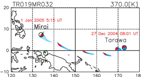
Fig. 1.Example of a cluster of trajectories leaving Tarawa. The blue and red dots are the whole segments calculated from the circled region with a match radius (1◦) centered at Tarawa. Only the red dots are included in both the first and second circular areas (i.e., those centered at Tarawa andMirai, respectively); therefore, they represent a match air parcel (see text for details). The footprints are drawn every 24 h. The air parcel observed over Tarawa on 27 December 2004 (first observation) was observed again (second ob-servation) overMiraiafter about 5 days.
are distributed more or less symmetrically with respect to the diagonal.
Fig. 2.Scatter plots showing the first (abscissa) versus the second observed values (ordinate) of ozone (left) and water vapor (right) mixing ratios for all preliminary matches connected by match air parcel. Color indicates the potential temperature. Bars in both pan-els indicate the uncertainties estimated by Hasebe et al. (2013), a companion paper to the present study. The dashed lines oriented parallel to the diagonal in the left panel indicate a difference of
±20 % between the paired observations, and the dotted curves indi-cate the range of±20 ppbv difference for the paired ozone mixing ratio. These are the thresholds of acceptable difference used in this study (see the last part of Sect. 3.3). Lines in the right panel indi-cate the accuracy of water vapor measurements; i.e.,±10 % (dashed lines) and±1 ppmv (dotted lines) (see Sect. 2). Note that the water vapor data measured by the Snow White hygrometers are not plot-ted above 360 K by their performance problem (see Sect. 2).
within the observational uncertainties for all the preliminary matches. Therefore, the distribution of data in these plots is near-spherical, as shown in the right panel of Fig. 3, thereby yielding a low correlation coefficient.
3.3 Screening of preliminary matches
The effectiveness of the methodology used to define prelim-inary matches is assessed using the ozone mixing ratio as a conserved property. In this section, we seek to screen out false matches before applying the match technique to dehy-dration in the TTL. The issues addressed by the screening procedure are the representativeness of the match air parcel, the degree of convective penetration, the validity of the isen-tropic treatment, and the consistency between sonde data and the analysis field.
3.3.1 Representativeness of match air parcel
A match air parcel that is composed of match air segments common to the first and second circular areas defined by a match radius (match air segments: see Sect. 3.2) must be rep-resentative of the circular area for both observations. Other-wise, the meteorological values measured at the first or sec-ond observations cannot be considered as those of a match air parcel. Consequently, it is important to examine the rep-resentativeness of the match air parcel. The representative-ness is examined based on the temperature difference be-tween the match air segments and whole segments included
Fig. 3.Left: As for the left panel in Fig. 2 but for preliminary matches for which the time interval between the first and second observations is less than 3 days (large circles). The small dots rep-resent all of the possible paired (see the text for details on the pairing procedure) observations (to reduce clutter, not all data are shown). Center: Correlation coefficients calculated for every 5 K of potential temperature (with±2.5 K bins) for the preliminary matches (red) and for all possible paired observations (blue). Error bars are 90 % confidence intervals. Right: As for the large circles in the left panel but for pairs at altitudes from 377.5 K to 382.5 K.
in the match circular area (see Appendix A1 for details). This assessment represents the first step of the screening proce-dure. To move on screening procedures for the remaining problems, we use the “conservative property of ozone” as the second principle. Note that these screening procedures are examined after the first step.
3.3.2 Convective penetration
The possible penetration of deep convection is diagnosed by comparing the temperatures of the match air segments (T) and the equivalent blackbody temperature of the underlying cloud (Tbb). If we assume monotonically decreasing
atmo-spheric temperature with increasing altitude, we may con-sider that the top of the convection is higher than the alti-tude of the advected air segment whenTbbminusT (≡δTbb)
is negative. However, it is well known that observed values of Tbb tend to overestimate the cloud top temperature; i.e.,
underestimate the cloud top altitude (e.g., Sherwood et al., 2004). To address this problem, we add some margin to
described below. If some deep convective clouds reach match air segments that advected in the TTL, some part of the seg-ments will be mixed with the tropospheric air mass, thereby changing the ozone mixing ratio. Thus, the degree of incon-sistency between the ozone mixing ratios at the first and sec-ond observations of a preliminary match could be used as an indicator of convective mixing. To statistically quantify such inconsistencies, we use the correlation coefficients between the ozone mixing ratios of the first and second observations as a function of the minimum value ofδTbbduring the
advec-tion. In this screening procedure, we adopt +12 K as the criti-cal value of the margin for the minimum value ofδTbbduring
the advection (see Appendix A2 for details). This margin cor-responds to 2.0–1.2 km in geometric height for a temperature lapse rate of 6–10 K km−1.
3.3.3 Validity of the isentropic treatment
Our trajectory calculations are made under the assumption of adiabatic conditions; however, this assumption becomes in-valid with increasing advection time, because radiative heat-ing or coolheat-ing occurs in the TTL dependheat-ing on the altitude and cloud conditions. Therefore, we need to establish an up-per limit of advection time that ensures the validity of the isentropic treatment and that is acceptable for our match analysis. This assessment is performed using a similar pro-cedure to that for convective penetration (Appendix A2). In other words, the correlation coefficients between the first and second observed ozone mixing ratios of preliminary matches are calculated as a function of the advection time of the match air parcels. We choose 5 days as the threshold of advection-time length (see Appendix A3 for details).
3.3.4 Consistency between sonde data and analysis field
The saturation water vapor mixing ratio (SMR) is estimated from the temperature field of the meteorological objective analysis (ECMWF data are used in this study) along the trajectories. Bias between the sonde data and analysis field would result in erroneous conclusions, including false ini-tialization of trajectory calculations. Inconsistencies between these factors could also arise from small-scale perturbations that are not resolved in the analysis field but are detected by sonde observations. We could reduce such differences by us-ing an isentropic coordinate system, because the air parcels stay on an isentrope even when displaced by small-scale tran-sient waves, such as gravity waves. However, temperature and pressure disturbances associated with the adiabatic mo-tion appear on the isentropes. If the temperature difference between the sonde and analysis field on the same potential temperature surface is large, then the dehydration process cannot be discussed by using both the water vapor mixing ratio measured by sonde and the saturation water vapor mix-ing ratio estimated from the analysis field. In addition, errors may exist in one or both of the data sets. Therefore, it is
im-portant to check for consistency between the sonde data and the analysis field. The consistency is assessed by calculat-ing the correlation coefficients between the first and second ozone mixing ratios of preliminary matches as a function of the difference in temperature between the ECMWF analysis and sonde data. We consider temperature differences of be-tween−4.0 and 5.0 K for assessing the consistency between the sonde data and analysis field (see Appendix A4 for de-tails). These temperature differences correspond to saturation water vapor mixing ratios of∼1 to∼6 ppmv in the TTL. 3.3.5 Other nonspecific factors
Finally, we re-check that ozone conservation does indeed oc-cur to screen out false matches caused by factors other than those examined above. In practice, the values that are equiv-alent to twice the uncertainty in ECC measurements (i.e., ±20 % or±20 ppbv; see also Sect. 2) are employed as the threshold of the acceptable difference in the ozone mixing ra-tio between the first and second observara-tions of each match.
4 Dehydration estimated from the matches
The water vapor match in the TTL is defined by trajec-tory calculations and the screening procedures described in Sect. 3. In this section, we discuss the amounts of water va-por change quantified from the matches. Figure 4 shows scat-ter plots of the first and second observations of the ozone and water vapor mixing ratios for 107 matches (i.e., all of the matches listed in Appendix B). Note that this number in-cludes matches of observational pairs and potential temper-ature levels. Among the 107 matches, there are 25 different observational pairs. The values for water vapor are similar between the first and second observations at potential tem-perature levels above 365 K (right panel), which suggests that the water vapor mixing ratios show little change. In turn, this means that we found no dehydrated cases in the altitude re-gion where the amount of water vapor entering the strato-sphere is controlled. The reasons why no such cases were found are discussed in Sect. 5.4. Below the 360 K level, al-most all of the cases show smaller water vapor amounts for the second observation than for the first. This result repre-sents the first piece of evidence from the water vapor match that appreciable dehydration occurred at these levels. In the following sections, the match cases are analyzed, focusing on hydration and dehydration during advection. Detailed case studies are presented in Sect. 4.1, while statistical features of the dehydration are derived in Sect. 4.2.
4.1 Detailed case studies
4.1.1 Case 1: water conserved
Fig. 4.As for Fig. 2 but for matches identified after applying all of the screening procedures (Sect. 3.3). In the right panel, the axes are modified compared with Fig. 2 and the symbols refer to the hy-grometers, i.e., crosses, triangles, and circles indicate paired obser-vations by CFH and CFH (for the first and second obserobser-vations, respectively), CFH and SW, and SW and SW, respectively.
(00:37 UT, 15 January 2007), both at Kototabang. The match air parcel advected for approximately 4 days at 371.0 K. The water vapor mixing ratios were measured by CFH, and the values are 3.1±0.3 ppmv for the first observation (left-hand red bar in b) and 3.4±0.3 ppmv for the second (right-hand red bar). Therefore, the water vapor amount was conserved during the advection. The histories of RHice, SMR, and
tem-perature of the advected match air parcel are shown in Fig. 5. Here, RHice and SMR are calculated using the water
va-por mixing ratio of the first measurement, assuming that the water vapor amount remains that of the first measurement. Figure 5a also shows the homogeneous freezing threshold (RHhom) according to K¨archer and Lohmann (2003), which
depends on the temperature of the match air parcel; this threshold is considered as the upper limit of RHice. The
dots in panel c are theTbb values of the underlying
atmo-sphere, corresponding to the advected air parcels. Isentropic backward trajectories, color-coded by the SMR, are shown in Fig. 5e. Figure 5d shows vertical profiles of water vapor observed at the first (orange) and second (red) sonde ob-servations, along with uncertainties. While the SMR of the match air mass, as estimated from the analysis field, reaches about 6.5 ppmv on the two days after the first observation, it is possible that the air mass experienced supersaturation on 11, 13, and 14 January 2007. The SMR during these peri-ods may have become smaller than the measured water vapor mixing ratio i.e., the RHice exceeds 100 %, although it does
not exceed RHhom. This SMR variation along the isentropic
trajectories is caused mainly by wave events rather than lat-itudinal motion (as is the case for the other matches). Be-cause this case is a match on a 371.0 K potential tempera-ture level, the screening procedure for convective penetra-tion (Appendix A2) is not applied. However, the values of
Tbb are appreciably larger than those of the match air mass
(≤195 K). In other words, the values ofTbbare high enough
to keep the air mass away from the area of convection.
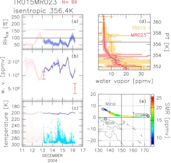
Fig. 5.Meteorological conditions of the match advecting from Ko-totabang (01:42 UT, 11 January 2007) to KoKo-totabang (00:37 UT, 15 January 2007) on the 371.0 K potential temperature surface. Those times correspond to the times of observations, i.e., 50 min after each launch (see Sect. 3.2). Vertical profiles of water vapor measured at the first (orange) and second (red) observations, along with esti-mates of errors, are shown in(d). The figure shows the time evo-lutions of (a)relative humidity over ice (RHice) on the
assump-tion that the water vapor amount is unchanged from the first mea-surement, along with the uncertainties (blue) and the homogeneous freezing threshold (RHhom; purple);(b)saturation water vapor
mix-ing ratio (SMR; blue line);(c)temperature (blue line) and equiva-lent black body temperature (Tbb; light blue dots); and(e)
trajec-tories of the match air parcel, color coded by SMR history. In(b), the superposed vertical bars in red are the water vapor mixing ratio measured at the match altitude (horizontal black line in(d)). Mete-orological data are from ECMWF, andTbbvalues are derived from
MTSAT-1R/GOES-9 IR images. For(a),(b),(c), and(e)each me-teorological value for the match air mass is superposed on that for the whole segments calculated from the circular region centered at the second observation (pink shading).
In this case, it is possible that the air mass was exposed to supersaturation during the advection, as described above, while the water vapor amount of the air mass was conserved. If we assume that nucleation of ice particles was not initiated at any period of the advection, the estimated maximum value of RHiceduring the advection is 124 % with an uncertainty of
−17 %/+16 % when the SMR becomes the minimum value (SMRmin), taking a value of 2.6 ppmv.
4.1.2 Case 2: dehydrated
surface with an advection time of about 3 days. The water va-por mixing ratios are 10.2±1.9 ppmv (the first observation) and 5.3±1.3 ppmv (the second), indicating some dehydra-tion during advecdehydra-tion.
In this altitude region, we find that the ECMWF tempera-ture has a cold bias of 2 K on the isentropic surfaces ranging from 355 to 360 K (Hasebe et al., 2013). For all subsequent analyses, this bias is taken into account when estimating SMR along the trajectories in this altitude region. The time evolution of SMR has small perturbations with an SMRmin
value of 8.9 ppmv at about 5 h before the second observa-tion. At this time, the temperature of the air mass is 197.4 K. This SMRminvalue is smaller than the water vapor mixing
ratio of the first observation. The RHiceduring advection
in-dicates a maximum value of RHice of 115 % with an
uncer-tainty of ±21 %. Because the match air mass is dehydrated, this case indicates that ice nucleation must have started be-fore the RHicereached 115 %. As this value is much smaller
than RHhom, it might correspond to the heterogeneous
freez-ing threshold. A comparison between the second water vapor observation and SMRmin suggests that dehydration
contin-ued until RHicereached 60 % with an uncertainty of ±16 %.
If the dehydration does not proceed to less than 100 % of RHice, the temperature of the air mass must have decreased
by about 3.2 K from the temperature 197.4 K, when the air mass is coldest, falling to 194.2 K on the 356.4 K potential temperature surface.
Information on the existence of ice particles is important when interpreting the RHice value in terms of dehydration
efficiency. For this purpose, we use the backscattering co-efficients observed by lidar installed on the research vessel Mirai. According to Fig. 3 of Fujiwara et al. (2009), cirrus clouds were observed at around the 355 K potential temper-ature level (about 15.5 km height) when the second obser-vation of this match was made. The cirrus clouds may have resulted from dehydration of the match air mass shown in Fig. 6, meaning that the match air mass may have experi-enced a temperature below 194.2 K.
4.1.3 Case 3: dehydrated
Figure 7 is the same as Fig. 5 but for the match from Biak (09:46 UT, 15 January 2008) to Hanoi (06:45 UT, 20 January 2008) on the 350.4 K potential temperature surface with an advection time of about 5 days. The observed water vapor mixing ratios are 37.7 ±5.6 ppmv (the first observation) and 17.5±1.9 ppmv (the second), indicating appreciable dehy-dration during advection.
This match air parcel has also experienced an SMR value smaller than the first observed water vapor mixing ratio. The SMRmin value of 15.1 ppmv is estimated just before
00:00 UT on 18 January 2008 (2.5 days after the first ob-servation). The RHiceshows a maximum value of 249 %, far
exceeding the RHhom, with an uncertainty of−37 %/+38 %
during the advection. Therefore, the match air parcel is
ex-Fig. 6.As for Fig. 5 but for the match that advected from Tarawa (03:48 UT, 13 December 2004) toMirai(05:17 UT on 16 December 2004) at the 356.4 K potential temperature surface with an advec-tion time of about 3 days.
pected to be dehydrated. The alternative comparison, be-tween the water vapor mixing ratio measured at the second observation and the SMRminvalue, yields an RHicevalue of
116 % with uncertainty of±12 % when the SMR attains the minimum value. This result suggests that the air mass was dehydrated down to 116 % RHicewhen the air mass
experi-enced SMRmin. The SMR history of this match air mass and
the water vapor mixing ratios observed at the first and sec-ond observations are discussed again in Sect. 5, along with a description of the procedure for estimating the efficiency of dehydration.
4.1.4 Case 4: hydrated
Fig. 7.As for Fig. 5 but for the match that advected from Biak (09:46 UT, 15 January 2008) to Hanoi (06:45 UT, 20 January 2008) at the 350.4 K potential temperature surface with an advection time of about 5 days.
Fig. 8.Vertical profiles of frost point temperature (red), temperature (black), and ozone mixing ratio (green) observed at Biak (04:35 UT, 16 January 2007). The horizontal bars show the uncertainties of sonde measurements estimated by Hasebe et al. (2013) (see ap-pendix A in their paper).
that deep convection penetrated into the TTL. However, it is puzzling in our case that the ozone mixing ratio (green) in Fig. 8 shows an increase with increasing altitude, reaching as high as 80 ppbv at the hydrated layer. Such a large amount of ozone is inconsistent with the idea that the air mass orig-inated from convection (Folkins et al., 2002). One possible explanation of the puzzling correlation between water vapor and the ozone profiles is that some convection is injected into an altitude above 380 K where the ozone profile has a local minima at the cold point, after which only ice particles fall to below the 380 K level and evaporate there.
Fig. 9.Scatter plot of ratios of the water vapor mixing ratio at the first observation to SMRminestimated from the SMR history during
advection (abscissa), versus ratios of the water vapor mixing ratio at the second observation to SMRmin(ordinate), for all matches.
Col-ors indicate the altitude (potential temperature). Symbols refer to the hygrometers (see the caption to Fig. 4). The dashed black lines indicate the approximate homogeneous freezing threshold (= 1.65).
4.2 Statistical features of dehydration
In Sect. 4.1, we used the matches to estimate the upper limit of RHice before ice condensation starts. This limit was
de-rived from the ratio of the first observed water vapor mixing ratio to SMRmin, as discussed using the dehydrated cases. In
this section, the statistical features of the dehydration in the TTL are examined.
Figure 9 shows a scatter plot of the ratio of the water va-por mixing ratio at the first observation to SMRminestimated
from the SMR history during the advection (abscissa), ver-sus the ratio of the water vapor mixing ratio at the second observation to SMRmin(ordinate), for all matches. The
col-ors indicate potential temperatures. The cases for which the water amount was conserved plot on the diagonal, while de-hydrated cases plot in the lower right part of the figure. The match cases for which the first (the second) water vapor mix-ing ratio coincides with SMRminappear on the black line
ori-ented vertically (horizontally).
Jensen and Pfister, 2004). The latter hydration process could not be detected in the present study, and is therefore not con-sidered further. The neglecting of this process is unlikely to significantly affect the results, because the absolute amount of water vapor generally shows an exponential decrease with decreasing temperature.
Below the 360 K level, on the other hand, many match pairs plot in the lower-right part of Fig. 9. Such air parcels encounter cold events in which SMRminis smaller than the
first observed water vapor mixing ratio (right-hand side of the vertical line), and are eventually dehydrated (lower right, near the diagonal).
It seems that the dehydration process differs between the lower and upper parts of the TTL.
The upper limit of RHice before ice nucleation starts and
that with ongoing dehydration has been estimated by us-ing all matches in which the match air parcel experienced saturation or supersaturation and then became dehydrated (i.e., cases in which the first observed water vapor amount is larger than both the second observed water vapor amount and SMRmin) in the altitude region from 350 to 360 K. For those
matches in which the maximum of RHice during the
advec-tion exceeds the RHhom, the value of RHhom is used except
for RHice because it is considered the upper limit of
saturation. A few cases experienced dehydration and super-saturation above 360 K; however, the number of cases is too small to enable a meaningful statistical analysis. The mean ratio of the water vapor mixing ratio at the first observation against SMRminis calculated to be 146±19 % (1σ) for cases
dehydrated below 360 K. The mean ratio of the water va-por mixing ratio at the second observation against SMRmin
is 75±23 % (1σ). The 1σ refers to the spread of results for different matches. These values suggest that the upper limit of RHice, before ice nucleation starts, is about 146 %, while
dehydration continues until RHicereaches, statistically, about
75 % in the altitude region from 350 to 360 K. The implica-tions of these values are discussed in Sect. 5.2.
5 Discussion
In general, tropical convective activities lift air masses from the planetary boundary layer to the level of neutral buoyancy. Above the approximately 400 K potential temperature sur-face, the Brewer–Dobson circulation lifts air masses to the deeper stratosphere. In the TTL, existing between these two regions, the air mass moves horizontally with a gradual as-cent balancing radiative heating. Rare detrainment of deep convective clouds may occur throughout the TTL, and this is likely to influence the water vapor concentrations of the TTL to some degree. The local temperature minimum in the TTL (approximately 370 K) over the western Pacific leads to cold trap dehydration. This dehydration process is considered to be the most important process controlling the amount of wa-ter vapor enwa-tering the stratosphere (e.g., Holton and
Get-telman, 2001; Hatsushika and Yamazaki, 2003; Fueglistaler et al., 2009; Hasebe et al., 2013).
A companion paper to the present study, Hasebe et al. (2013), conducted a statistical analysis of the relationship between the observed water vapor mixing ratio and the mini-mum saturation water vapor mixing ratio that the air mass ex-perienced in the past five days. The results showed that cold trap dehydration progressed with slow diabatic ascent from 360 K to 380 K. In the present study, it is unfortunate that de-hydrated air masses are rare in the altitude region around the 370 K potential temperature surface (the reasons for this are discussed in Sect. 5.4); nonetheless, dehydration associated with horizontal advection is evident in the lower part of the TTL, as revealed by the match technique. The following sec-tion discusses the applicability of the screening parameters examined in Sect. 3.3, the two RHicevalues evaluated as the
ratios of the first- and second-observed water vapor mixing ratios against SMRminin the previous section, the efficiency
of dehydration in the lower TTL, and the lack of dehydrated cases near the cold point.
5.1 Applicability of screening parameters
In this study, several numerical values of the screening cri-teria were examined and estimated as screening parameters (Sect. 3.3 and Appendix A). Here, we consider whether the parameters estimated in this study could be applied to other TTL studies that consider different regions or seasons.
with satellite zenith angle around 50◦is less than 1 km. This difference is not statistically significant, according to Fig. 7 in Hamada and Nishi (2010). Therefore, the criterion for “convective penetration” (i.e.,< δTbb>min≥12 K; see
Ap-pendix A2) may be applied to studies in different regions and seasons. However, the numerical value of the criterion should be re-evaluated when usingTbbdata with different resolution
from that of MTSAT-1R/GOES-9, such as data observed by MODerate resolution Imaging Spectroradiometer (MODIS). 5.2 Relative humidity before ice nucleation and after
dehydration in the lower TTL
As described in Sect. 4.2, the upper limit of RHice before
the initiation of condensation is estimated to be 146±19 % (1σ) from matches, indicating dehydration in the altitude range from 350 to 360 K in potential temperature. These es-timates are based on a meteorological analysis field having finite temporal–spatial resolution; hence, sub-grid-scale vari-ations are not taken into account. It is possible that the air is instantaneously exposed to a higher degree of supersatura-tion than that estimated in the present study. Comparisons of the second observed water mixing ratio and SMRmin yield
an estimate of the air masses being dehydrated to the level of RHice reaching 75±23 % (1σ). If we take this result at
face value, TTL dehydration could proceed beyond the ap-parent saturation level, although the estimated uncertainty is too large to be certain of this possibility. Statistically this level of significance is not large enough to claim that the threshold is below 100 %. Therefore, although the derived value is far from 100 % RHice, the significance is not strong
enough to claim that ice growth happens at subsaturated con-ditions. However, one possible explanation of ice growth un-der unsaturated conditions is that the value of our estimate is affected by sub-grid-scale temperature perturbations that could not be resolved in our analysis, as described above. For example, temperature variation of 2 K is sufficient to create RHice variation of up to 30 %.
Some studies (e.g., Voigt et al., 2008; Chepfer and Noel, 2009) raised the possibility that nitric acid trihydrate (NAT; HNO3–3H2O) exists in the TTL. Crutzen and Arnold (1986)
show that the critical temperature of NAT formation is higher than that of ice formation. In such a case, although the inter-pretation of our results would become even more complex, it may be possible that the dehydration could progress to a state
the abundance of HNO3is much smaller than that of H2O in
the TTL. Therefore, even if NAT particles were formed and fully removed from the air mass, they would remove only a few ppbv of water vapor, which is insignificant with respect to dehydration.
Given that our estimates of the initiation and termination of ice nucleation have large uncertainties, there is little that we can infer from the results. However, by accumulating more matches with improved accuracy of both observations and trajectory calculations, it would be possible to improve our understanding of the conditions required for ice nucle-ation.
5.3 Estimation of the efficiency of dehydration in the lower TTL
The efficiency of dehydration depends on various factors, in-cluding the concentration and size distribution of cloud con-densation nuclei, the duration of a cold event, and the degree of supersaturation of the air mass. Although a complete set of observations is unavailable, our matches would provide some useful constraints on the processes of dehydration in the TTL. We attempt to model the efficiency of dehydration using two terms: the critical value of RHice that enables ice
nucleation (RHcri) and the dehydration rate as a gross
mea-sure of the nucleation rate and the gravitational removal of ice particles. Here, the dehydration rate is defined as the re-laxation time (e-folding time:τ [hour]) taken by a supersat-urated air parcel to approach the saturation state by the nu-cleation and removal of ice particles. These two parameters, RHcri andτ, are estimated as follows. Suppose that an air
mass with the water vapor mixing ratio of the first observa-tion advects along the trajectories. If the parameters RHcri
andτ are given, we would describe the time evolution of the water vapor mixing ratio for each advected air parcel. For example, in the case of RHcri= 110 %, the air mass starts
to be dehydrated, with the rate of dehydration depending on
τ when the RHice exceeds 110 %. Such calculations are
re-peated for a given value of RHcri (values of 100 %, 110 %,
130 %, and 165 %) to identify the value ofτ that is consis-tent with the second observation of water vapor. These val-ues of RHcri correspond to the water saturation,
(a)
(b)
(c)
(d)
Fig. 10.Dehydration scenarios showing the time evolution of the water vapor mixing ratio of the air mass (red line) and exposed SMR (blue line) estimated from the match case shown in Fig. 7. The value ofτstated in each panel is the estimated relaxation time of conden-sation for the assumed values of RHcri, which are(a)100 %,(b)
110 %,(c)130 %, and(d)165 %.
temperature and pressure, and it is assumed to have a fixed value during advection.
Figure 10 shows examples for such calculations corre-sponding to the match air parcel shown in Fig. 7. For a RHcri
value of 100 %, it is evident that the air mass is dehydrated every time the SMR becomes smaller than the water vapor it contains (Fig. 10a). On the other hand, dehydration does not occur in other cases until some additional cooling is ap-plied. In most cases (but not all), we find a unique value of
τ that best fits the second water vapor observation for any
given value of RHcri. Of note, no value ofτ yields the
sec-ond observed water vapor mixing ratio for a RHcrivalue of
near 165 % (Fig. 10d).
The statistical features of the efficiency of dehydration are analyzed in terms of the values of RHcriandτ. Table 2 shows
the variation inτ for each RHcrivalue derived from matches.
τ shows a general decrease with increasing RHcri, although
there are exceptions. Below 360 K, the mean values ofτ are approximately 1.0 h in the cases supposing a heterogeneous threshold, regardless of RHcri. These values are much shorter
than the typical timescale of horizontal advection in the TTL, and are shorter than the time interval of available ECMWF data. Therefore, it is suggested that cold trap dehydration is quite efficient in the lower levels of the TTL. On the other hand, values of τ are estimated to be more than 100 h at 369 K for the RHcrivalues other than 165 %. This raises the
possibility that the value ofτ increases in the upper levels of the TTL.
Naturally, the species of aerosols control the cloud-microphysical behavior of the atmosphere. However, the value ofτ was calculated for an assumed RHcriand after the
beginning of ice nucleation, thereby depending on the value of assumed RHcri. In addition, the value ofτ is largely
inde-pendent of the value of RHcri, as shown in Table 2. Therefore,
the estimate ofτis unlikely to show marked changes with the background aerosol condition. However, it may be sensitive to the altitude range, as indicated by the facts that values of
τ are estimated to be more than 100 h at 369 K and that de-hydrated cases are lacking near the cold point (the possible reason for this is discussed in Sect. 5.4).
5.4 Lack of dehydrated cases near the cold point
trajectory calculation in order to track the air mass for long enough to enable the dehydration to reach completion.
The ice number concentration and the particle size of cirrus clouds in the TTL are reported to be approximately 100 L−1and 10 µm, respectively (e.g., Shibata et al., 2007; Kr¨amer et al., 2009). Such a water content is equal to ap-proximately 0.5–1.0 ppmv of the water vapor mixing ratio in the TTL environment. According to Pruppacher and Klett (1997), an ice particle of 10 µm in size requires approxi-mately 8 h to fall through 1 km. However, these values cor-respond to cirrus clouds with a relatively thick optical depth; in contrast, the ice particles in optically thin cirrus clouds are much smaller than 10 µm. For example, Pruppacher and Klett (1997), stated that a particle of 1 µm in size (the exis-tence of such small ice particles was suggested by Iwasaki et al., 2007) requires approximately 20 days to fall through 1 km. If the dehydration process around the cold point results in the formation of such small particles, then the period re-quired for ice removal is too long to enable tracking of the air parcel. Unfortunately, such a long-running trajectory would be difficult to calculate accurately and it would be inappro-priate for match analysis; in addition, it could be used to es-timate the global-scale distribution of water vapor, as shown by Fueglistaler et al. (2004) and Ploeger et al. (2011).
If the lack of dehydrated cases around the cold point re-flects the fact that the dehydration timescale is too long, one effective approach to resolve this problem would be to re-duce the uncertainty in water vapor measurements and to ob-serve the size distribution and concentration of ice particles together with the amount of water vapor. Because the default soundings in previous SOWER campaigns did not include any sensors for particles, we could not estimate the total wa-ter content in which the air mass has ice particles. In addi-tion, for the campaign region and period (i.e., over the west-ern Pacific in the boreal winter), cirrus clouds are common in the TTL; Shibata et al., 2007; Fujiwara et al., 2009; Massie et al., 2010; Yang et al., 2010; Inai et al., 2012; Shibata et al., 2012). If we could observe ice particles and measure their concentration and size distribution, we could estimate their growth rate under the assumption that a critical relative hu-midity leads to the initiation of ice nucleation, using the same technique as that employed to estimate the efficiency of de-hydration (Sect. 5.3). The history of relative humidity of the air mass could be estimated by using the match method
to-gether with the meteorological history of the match air mass. Estimations of growth rate, as well as measurements of the size distribution of ice particles, would enable estimates of the time evolution of the falling speed of ice particles with respect to the surrounding atmosphere. In addition, if we con-firm or assume that no ice particles fall from the upper layer, we can estimate the net removal rate of water vapor from the match air parcel. Estimations of these parameters would pro-vide a quantitative description of the efficiency of cold trap dehydration.
6 Conclusions
This study investigated evidence for, and the efficiency of, dehydration associated with horizontal advection strato-sphere. The water vapor match in the TTL was developed by trajectory calculations with intensive screening procedures to reduce the uncertainty in the results.
The matches were identified by using screening proce-dures. Some of the matches indicated a decrease in the amount of water vapor between the first and second obser-vations of the water vapor mixing ratio. This finding repre-sents the first direct evidence of dehydration associated with horizontal advection in the TTL.
Fig. A1.Representativeness of the match air parcel at Tarawa (top: 05:09 UT, 31 December 2005) and Biak (bottom: 01:49 UT, 6 Jan-uary 2006). These preliminary matched observations are connected by trajectories at the 355.8 K potential temperature surface. Left: Match air segments (diamonds) superposed on color-coded temper-ature of the circular area defined by a match radius. Right: Temper-ature frequency distribution of the whole segments within the cir-cular area defined by a match radius (black bars) and that for match air segments (red bars).
the lower part of the TTL. These findings may improve our understanding of cloud-microphysical processes in the TTL. The matches that indicate dehydration were not found at altitudes close to the cold point tropopause (i.e., potential temperature ranging from 370 to 380 K). Given that the de-hydration around this level determines the amount of water vapor entering the stratosphere, and to improve on the statis-tical results from this study, additional observation data and more match events at this level are required.
Appendix A
Detailed descriptions of screening procedures
A1 Representativeness of the match air parcel
The match air parcels must be representative of a certain area; otherwise, the values observed by the sonde are not con-sidered as those of the match air parcel. Figure A1 shows the horizontal distribution (left) and frequency distribution (right) of temperature in the match circular areas correspond-ing to the sonde observations at Tarawa (top) and Biak
(bot-Fig. A2.As for Fig. A1 but for the preliminary match at Biak (top: 22:50 UT, 18 January 2006) and Hanoi (bottom: 06:57 UT, 21 Jan-uary 2006) on the 350.2 K potential temperature surface.
tom) on the 355.8 K potential temperature surface. These match air segments are the origins of the forward (backward) trajectories in the upper (lower) panel. In this case, the tem-perature fields in the circular regions with a match radius for the first and second observations are almost uniform. In addi-tion, the match air segments are widely distributed, covering the match circular areas. Therefore, these match air segments are representative of the temperatures inside both match cir-cles. The confidence intervals of the mean temperature differ-ence between the match air segments and the whole segments inside the match circle are from−0.02 to 0.03 K for the first observation (Fig. A1 (top)) and from 0.12 to 0.19 K for the second observation (Fig. A1 (bottom)) at a significance level of 0.1. The intervals were calculated using Welch’s test statis-tic (see Appendix B).
Fig. A3.Match air segments (red area at∼2◦S,∼164◦E) similar to the red dots in Fig. 1 superposed on the distribution ofTbb(color)
at 06:00 UT on 29 December 2004. The black circles show the cir-cles of the match radius (1◦) centered at individual observational stations.
According to the screening procedure adopted in this study, observational pairs are rejected if the confidence in-terval of the mean temperature difference between the match air segments and the whole segments inside the match cir-cle does not fall within [-2.0, 2.0] K for the first and second observations at a significance level of 0.1. This temperature range is determined empirically; the temperature difference of 2.0 K corresponds to a difference in the saturation water vapor mixing ratio in the TTL of∼0.5 to∼2.0 ppmv. A2 Convective penetration
To diagnose convective penetration into the match air parcel, the temperatures of the match air segments (T) and the equiv-alent blackbody temperature of the underlying cloud (Tbb)
are compared, and the value ofTbbminusT (≡δTbb) is
de-fined. The values ofTbbare estimated from hourly
MTSAT-1R/GOES-9 infrared images (Channel 1: 10.3–11.3 µm). Fig-ure A3 shows an example of advected match air segments similar to the red dots in Fig. 1, superposed on theTbb
distri-bution at 06:00 UT on 29 December 2004.
To determine an appropriate margin forδTbbin diagnosing
the penetration of deep convection, the values of< δTbb>
are calculated as the average for the smallest 10th percentile ofδTbb values of the air segments constituting the match air
parcel for each time step. Then, the values of< δTbb>min
for each match air parcel are defined as the minimum value of < δTbb> during the advection. Finally, the correlation
coefficients of the ozone mixing ratio between the first and second paired observations are calculated as a function of
< δTbb>min. The bins are established with a range of±2.5 K
and an increment of 1.0 K. The left panel of Fig. A4 shows a scatter plot of the first versus the second observed ozone mixing ratios color-coded by each value of < δTbb>min.
Light purple symbols indicate preliminary matches above 370 K that are not used in this procedure, as described below. The correlation coefficients decrease with decreasing values of< δTbb>min. The correlation coefficients are high when
the values of < δTbb>min are higher than +12 K.
There-Fig. A4.Examination of convective penetration for the match pairs. Left: Scatter plot of the first versus the second ozone mixing ra-tios for preliminary matches that passed the screening for “rep-resentativeness of match air parcel” color-coded by the value of
< δTbb>min(see text for details). Right: Dependency of
correla-tion coefficients for ozone mixing ratios between the first and sec-ond observations on the value of< δTbb>min. The error bars are 99 % confidence intervals.
fore, we adopt +12 K as the critical value of the margin for
< δTbb>min.
This method cannot be applied to air segments advected above the temperature inversion at the cold point, as the dis-tance between the air parcel and underlying cloud cannot be estimated from the comparison of T andTbb at those
lev-els. Although some deep convection penetrates the strato-sphere up to the 420 K isentropic level (Khaykin et al., 2009; Iwasaki et al., 2010) on rare occasions, we do not apply the screening procedure to air parcels above the 370 K potential temperature level. Instead, the matches above the 370 K level that pass all the screening steps are carefully checked with reference to individual sonde profiles (see Sect. 4.1).
An alternative method to diagnose convective penetration, such as that used by Suzuki et al. (2010) employing cloud top height data by Hamada and Nishi (2010), is not used in the present analysis because the data set does not fully cover the SOWER campaign period and region.
A3 Validity of the isentropic treatment
Fig. A5.As for Fig. A4 but for an examination of the acceptable advection time for the isentropic treatment.
The right panel of Fig. A5 shows the dependency of the cor-relation coefficients of ozone mixing ratios between the first and second observations on advection time. The correlation coefficients are calculated using the data in the left panel us-ing bins of±1.0 day with an increment of 0.5 days depending on the advection time of each match air parcel. The correla-tion coefficients decrease as the adveccorrela-tion time increases, due to the cumulative effect of errors in the isentropic trajectory calculations. In this study, we choose 5 days as the threshold of advection time, since the minimum value of the correlation coefficients is found at 5.5 days.
A4 Consistency between sonde data and the analysis field
The criterion employed in the screening procedure for con-sistency between the sonde data and the analysis field is assessed by considering the difference in temperature be-tween the ECMWF analysis and sonde data:TECMWFminus
T (≡δT) at the same potential temperature surface. Here,
TECMWFis the temperature of the ECMWF analysis field
in-terpolated to the location of the sonde station at 50 min af-ter the launch. This assessment is also performed by using a similar method to those outlined in Appendices A2 and A3; i.e., employing the correlation coefficients between the first and second ozone mixing ratios. In this examination, the cor-relation coefficients are calculated as a function ofδT with bins of±1.0 K and an increment of 0.5 K. This procedure is conducted for both the first and second observations for each preliminary match. Figure A6 is the same as Fig. A5 but ex-amines the consistency between sonde data and the analysis field. The data in the left panel are color-coded by values ofδT. The preliminary matches above the 380 K isentrope are not used in this procedure, for the same reason as that explained in Appendix A3. The right panel shows the de-pendency of the correlation coefficients on δT. There is a broad maximum around zero, although some asymmetry is apparent. There are remarkable decreases in the correlation coefficient at−5.0 and +6.0 K, and we cannot explain the
re-Fig. A6.As for Fig. A5 but for examining the consistency between sonde data and the analysis field.
covery in values outside of these limits. To assure a relatively high correlation between the paired ozone concentrations, we adopt a range of temperature differences between−4.0 and 5.0 K as the criterion for assessing the consistency between sonde data and the analysis field.
Appendix B
Welch’s test statistic
Welch’st-test defines the statisticT as follows:
T =qx¯1− ¯x2 s12 N1 +
s22 N2
, (B1)
where (x¯1,x¯2), (s1, s2), and (N1, N2) indicate the mean
val-ues, the standard deviations, and the numbers of first and second samples, respectively. This T value follows the t -distribution corresponding to the degree of freedomm cal-culated from
m=
s12 N1 +
s22 N2
2
s14 N12(N1−1)
+ s24 N22(N2−1)
. (B2)
Referring to this value, the confidence interval of the differ-ence between the two population means (µ1−µ2) is
esti-mated from the following:
(x¯1− ¯x2)−tm α
2
s
s12
N1
+s2
2
N2
≤µ1−µ2≤(x¯1− ¯x2)
+tm α
2
s
s12
N1
+s2
2
N2
, (B3)
TR015 MR023 354.8 TR015 MR023 355.0 TR015 MR023 355.2 TR015 MR023 355.4 TR015 MR023 355.6 TR015 MR023 355.8 TR015 MR023 356.0 TR015 MR023 356.4 TR015 MR023 356.6 TR015 MR023 356.8 BD218 BD219 361.0 BD218 BD219 377.0 TR029 TR030 352.4 TR029 TR030 352.6 TR029 TR030 352.8 TR029 TR030 353.0 TR029 TR030 353.2 TR029 TR030 353.4 TR029 TR030 353.6 TR029 TR030 353.8 TR029 TR030 354.0 TR029 TR030 356.4 TR029 TR030 356.6 TR029 TR030 356.8 TR029 TR030 357.0 TR029 TR030 357.2 TR029 TR030 357.4 TR029 TR030 357.6 BI028 HN062 355.4 HN061 TR052 361.0 KT023 KT025 369.0 KT023 KT025 370.0 KT023 KT025 371.0 KT023 KT025 372.0 KT023 KT025 373.0 KT023 KT025 374.0 BI030 BI031 377.0 BI030 BI031 378.0 BI030 BI032 378.0 BI030 BI032 379.0 BI029 BI030 379.0 BI029 BI030 380.0 BI029 BI030 381.0 BI029 BI031 379.0 BI031 BI032 379.0 BI031 BI032 380.0 BI031 BI032 381.0 BI031 BI032 382.0 BI031 BI032 383.0 BI028 BI030 384.0 BI028 BI030 385.0 BI028 BI030 386.0
TR051 TR054 391.0
KT022 KT023 387.0
KT022 KT023 388.0
KT022 KT023 389.0
KT022 KT023 390.0
KT022 KT023 391.0
KT022 KT023 392.0
KT022 KT023 393.0
KT022 KT023 394.0
KT022 KT023 395.0
KT022 KT023 396.0
KT022 KT023 397.0
KT022 KT023 398.0
KT022 KT023 399.0
KT022 KT023 400.0
BI027 BI028 391.0
BI027 BI028 392.0
BI027 BI028 393.0
BI027 BI028 394.0
BI027 BI028 395.0
TR053 TR054 392.0
TR053 TR054 393.0
TR053 TR054 394.0
KT024 KT025 400.0
BI039 HN093 350.4
BI039 HN093 352.4
KT031 KT032 391.0
KT031 KT032 392.0
KT031 KT032 393.0
KT031 KT032 394.0
BI037 KT034 364.0
BI036 KT034 387.0
BI036 KT034 388.0
BI036 KT034 389.0
BI036 KT034 390.0
BI036 KT034 391.0
BI038 BI039 396.0
BI037 BI038 395.0
BI037 BI038 396.0
BI037 BI038 397.0
BI037 BI038 398.0
BI037 BI038 399.0
BI037 BI038 400.0
BI037 BI039 396.0
BI037 BI039 397.0
BI037 BI039 398.0
BI037 BI039 399.0
Acknowledgements. The authors are grateful to the members of Lembaga Penerbangan dan Antariksa Nasional (LAPAN) of Indonesia, the Meteorological Office of Tarawa, Kiribati, and the Aero-Meteorological Observatory of Hanoi, Vietnam. We also thank the Japan Agency for Marine-Earth Science and Technology (JAMSTEC) and Global Ocean Development, Inc. (GODI) for their support on board the R/VMirai. This work was supported by KAKENHI, Japan Society for the Promotion of Science, Japan (15204043, 16740264, 18204041, 21244072, and 22241004) and by the Global Environment Research Fund of the Ministry of the Environment, Japan (A-1 and A-071). GOES-9 and MTSAT-1R data were obtained from Kochi University, Japan. The figures were produced by the GFD-DENNOU Library. Comments by S. Fueglistaler and two anonymous reviewers helped to improve the manuscript.
Edited by: G. Stiller
References
Brasseur, G. and Solomon, S.: Aeronomy of the Middle Atmo-sphere: Chemistry and Physics of the Stratosphere and Meso-sphere, Dordrecht, Boston, 1986.
Chepfer, H. and Noel, V.: A tropical “NAT-like” belt
ob-served from space, Geophys. Res. Lett., 36, L03813,
doi:10.1029/2008GL036289, 2009.
Corti, T., Luo, B. P., Fu, Q., V¨omel, H., and Peter, T.: The impact of cirrus clouds on tropical troposphere-to-stratosphere transport, Atmos. Chem. Phys., 6, 2539–2547, doi:10.5194/acp-6-2539-2006, 2006.
Crutzen, P. J. and Arnold, F.: Nitric acid cloud formation in the cold Antarctic stratosphere: a major cause for the springtime “ozone hole”, Nature, 342, 651–655, 1986.
Dessler, A. E.: The effect of deep, tropical convection on the tropical tropopause layer, J. Geophys. Res., 107, 4033, doi:10.1029/2001JD000511, 2002.
Folkins, I., Braun, C., Thompson, A., and Witte, J.: Tropical ozone as an indicator of deep convection, J. Geophys. Res., 107, 4184, doi:10.1029/2001JD001178, 2002.
Forster, P. M. d. F. and Shine, K. P.: Stratospheric water vapour changes as a possible contributor to observed stratospheric cool-ing, Geophys. Res. Lett., 26, 3309–3312, 1999.
Fueglistaler, S., Wernli, H., and Peter, T.: Tropical troposphere-to-stratosphere transport inferred from trajectory calculations, J. Geophys. Res., 109, D03108, doi:10.1029/2003JD004069, 2004. Fueglistaler, S., Bonazzola, M., Haynes, P. H., and Peter, T.: Strato-spheric water vapor predicted from the Lagrangian temperature history of air entering the stratosphere in the tropics, J. Geophys. Res., 110, D08107, doi:10.1029/2004JD005516, 2005.
Fueglistaler, S., Dessler, A. E., Dunkerton, T. J., Folkins, I., Fu, Q., and Mote, P. W.: TROPICAL TROPOPAUSE LAYER, Rev. Geo-phys., 47, RG1004, doi:10.1029/2008RG000267, 2009. Fujiwara, M., Shiotani, M., Hasebe, F., V¨omel, H., Oltmans, S. J.,
Ruppert, P. W., Horinouchi, T., and Tsuda, T.: Performance of the Meteolabor “Snow White” chilled-mirror hygrometer in the tropical troposphere: Comparisons with the Vaisala RS80 A/H-Humicap sensors, J. Atmos. Ocean. Technol., 20, 1534–1542, 2003.
Fujiwara, M., Iwasaki, S., Shimizu, A., Inai, Y., Shiotani, M., Hasebe, F., Matsui, I., Sugimoto, N., Okamoto, H., Nishi, N., Hamada, A., Sakazaki, T., and Yoneyama, K.: Cirrus Observa-tions in the Tropical Tropopause Layer Over the Western Pacific, J. Geophys. Res., 114, D09304, doi:10.1029/2008JD011040, 2009.
Fujiwara, M., V¨omel, H., Hasebe, F., Shiotani, M., Ogino, S.-Y., Iwasaki, S., Nishi, N., Shibata, T., Shimizu, K., Nishi-moto, E., Canossa, J. M. V., Selkirk, H. B., and Oltmans, S. J.: Seasonal to decadal variations of water vapor in the tropical lower stratosphere observed with balloon-borne cryo-genic frost point hygrometers, J. Geophys. Res., 115, D18304, doi:10.1029/2010JD014179, 2010.
Gill, A. E.: Some simple solutions for heat-induced tropical circu-lation, Q. J. R. Meteorol. Soc., 106, 447–462, 1980.
Goff, A. J. and Gratch, S.: Low-pressure properties of water from –160 to 212◦F, Trans. Amer. Soc. Heat. Vent. Eng., 52, 95–122, 1946.
Hamada, A. and Nishi, N.: Development of a Cloud-Top Height Es-timation Method by Geostationary Satellite Split-Window Mea-surements Trained withCloudSatData, J. Appl. Meteor. Clima-tol., 49, 2035–2049, doi:10.1175/2010JAMC2287.1, 2010. Hasebe, F., Fujiwara, M., Nishi, N., Shiotani, M., V¨omel, H.,
Olt-mans, S., Takashima, H., Saraspriya, S., Komala, N., and Inai, Y.: In situ observations of dehydrated air parcels advected hori-zontally in the Tropical Tropopause Layer of the western Pacific, Atmos. Chem. Phys., 7, 803-813, doi:10.5194/acp-7-803-2007, 2007.
Hasebe, F., Inai, Y., Shiotani, M., Fujiwara, M., V¨omel, H., Nishi, N., Ogino, S.-Y., Shibata, T., Iwasaki, S., N.Komala, Peter, T., and Oltmans, S. J.: Cold trap dehydration in the tropical tropopause layer characterized by SOWER chilled-mirror hy-grometer network data in the Tropical Pacific, Atmos. Chem. Phys., 13, 4393–4411, doi:10.5194/acp-13-4393-2013, 2013. Hatsushika, H. and Yamazaki, K.: Stratospheric drain over
Indone-sia and dehydration within the tropical tropopause layer diag-nosed by air parcel trajectories, J. Geophys. Res., 108, 4610, doi:10.1029/2002JD002986, 2003.
Highwood, E. J. and Hoskins, B. J.: The tropical tropopause, Q. J. Roy. Meteorol. Soc., 124, 1579–1604, 1998.
Holton, J. R. and Gettelman, A.: Horizontal transport and the dehy-dration of the stratosphere, Geophys. Res. Lett., 28, 2799–2802, 2001.
Hurst, D. F., Oltmans, S. J., V¨omel, H., Rosenlof, K. H., Davis, S. M., Ray, E. A., Hall, E. G., and Jordan, A. F.: Strato-spheric water vapor trends over Boulder, Colorado: Analysis of the 30 year Boulder record, J. Geophys. Res., 116, D02306, doi:10.1029/2010JD015065, 2011.
Inai, Y., Hasebe, F., Shimizu, K., and Fujiwara, M.: Correc-tion of Radiosonde Pressure and Temperature Measurements Using Simultaneous GPS Height Data, SOLA, 5, 109–112, doi:10.2151/sola.2009-028, 2009.
Inai, Y., Shibata, T., Fujiwara, M., Hasebe, F., and V¨omel, H.: High supersaturation inside cirrus in well-developed tropi-cal tropopause layer over Indonesia, Geophys. Res. Lett., 39, L20811, doi:10.1029/2012GL053638, 2012.