Agnotology: learning from mistakes

(1)

ESDD

4, 451–505, 2013

Agnotology: learning from mistakes

R. E. Benestad et al.

Title Page

Abstract Introduction

Conclusions References

Tables Figures

◭ ◮

Back Close

Full Screen / Esc

Printer-friendly Version Interactive Discussion

Discussion

P

a

per

|

Dis

cussion

P

a

per

|

Discussion

P

a

per

|

Discussio

n

P

a

per

|

Earth Syst. Dynam. Discuss., 4, 451–505, 2013 www.earth-syst-dynam-discuss.net/4/451/2013/ doi:10.5194/esdd-4-451-2013

Open Access

Earth System Dynamics

Discussions

Geoscientiic Geoscientiic

This discussion paper is/has been under review for the journal Earth System Dynamics (ESD). Please refer to the corresponding final paper in ESD if available.

Agnotology: learning from mistakes

R. E. Benestad1, H. O. Hygen1, R. van Dorland2, J. Cook3, and D. Nuccitelli4

1

The Norwegian Meteorological Institute, Norway 2

The Royal Netherlands Meteorological Institute, The Netherlands 3

Global Change Institute, the University of Queensland, Australia 4

Tetra Tech, Inc., McClellan, California, USA

Received: 4 April 2013 – Accepted: 22 April 2013 – Published: 3 May 2013

Correspondence to: R. E. Benestad (rasmus.benestad@met.no)

(2)

ESDD

4, 451–505, 2013

Title Page

Tables Figures

◭ ◮

Back Close

Full Screen / Esc

Discussion

P

a

per

|

Dis

cussion

P

a

per

|

Discussion

P

a

per

|

Discussio

n

P

a

per

|

Abstract

Replication is an important part of science, and by repeating past analyses, we show that a number of papers in the scientific literature contain severe methodological flaws which can easily be identified through simple tests and demonstrations. In many cases, shortcomings are related to a lack of robustness, leading to results that are not

univer-5

sally valid but rather an artifact of a particular experimental set-up. Some examples presented here have ignored data that do not fit the conclusions, and in several other cases, inappropriate statistical methods have been adopted or conclusions have been based on misconceived physics. These papers may serve as educational case studies for why certain analytical approaches sometimes are unsuitable in providing reliable

10

answers. They also highlight the merit of replication. A lack of common replication has repercussions for the quality of the scientific literature, and may be a reason why some controversial questions remain unanswered even when ignorance could be reduced. Agnotology is the study of such ignorance. A free and open-source software is pro-vided for demonstration purposes.

15

1 Introduction

Bedford (2010) argued that “agnotology” (the study of how and why we do not know things) presents a potentially useful tool to explore topics where knowledge is or has

been contested by different people. The term “agnotology” was for the first time coined

in Proctor and Schiebinger (2008), which provided a collection of essays addressing

20

the question “why we do not know what we do not know?”. Their message was that ignorance is a result of both cultural and political struggles as well as an absence of knowledge. The counterpart to agnotology is epistemology, for which science is an important basis. In principle, the scientific way of thinking is the ideal means of resolv-ing questions about causality, and science can provide valuable guidance when there

25

(3)

ESDD

4, 451–505, 2013

Title Page

Tables Figures

◭ ◮

Back Close

Full Screen / Esc

Discussion

P

a

per

|

Dis

cussion

P

a

per

|

Discussion

P

a

per

|

Discussio

n

P

a

per

|

virtues is debate and disagreement about different hypotheses, making it dynamic and

providing a driving force for progress. In this process, controversial questions should be addressed with the scientific method and rigour, and in order to provide convinc-ing answers, it is important that the process is transparent, the results are replicable, the hypotheses testable, and the tests objective. It is also important that critiques and

5

debates are conveyed by the scientific literature when past findings are challenged. An agnotological study of the climate sciences can shed light on some recent

contro-versies which take place when groups with di_fferent scientific backgrounds and

mind-sets dispute each other’s conclusions. Some case studies may include a number of recent papers that have suggested a strong influence on Earth’s climate from solar

vari-10

ability, Jupiter, Saturn or the lunar orbit (Friis-Christensen and Lassen, 1991; Scafetta, 2010; Scafetta and West, 2008, 2007, 2006a, b, 2005; Svensmark, 1998; Svensmark and Friis-Christensen, 1997). These papers have also argued that greenhouse gases

(GHG) such as CO₂play a relatively small role for Earth’s climate, and dispute the view

presented by the mainstream climate research community (National Research Council

15

(US), 2001; Oreskes, 2004; Solomon et al., 2007). In this respect, it is important to ask

whether these differences reflect legitimate uncertainties and gaps in our knowledge. In

order to get to the bottom of such issues, one needs to follow the line from the original information source, via analysis, to the interpretation of the results and the final con-clusions. True and universal answers should in principle be replicated independently,

20

especially if they have been published in the peer reviewed scientific literature. A mes-sage from Proctor and Schiebinger (2008) is that ignorance in these issues may stem from the culture neglecting replication, not sharing methods and data, or not testing

the methods in di_fferent settings. The most persuasive arguments are the ones where

everybody can repeat the analyses for themselves, examine the methods, and get the

25

same results. Scientific truths should in principle be universal, which means that they should be generally valid and the methods objective.

(4)

ESDD

4, 451–505, 2013

Title Page

Tables Figures

◭ ◮

Back Close

Full Screen / Esc

Discussion

P

a

per

|

Dis

cussion

P

a

per

|

Discussion

P

a

per

|

Discussio

n

P

a

per

|

taken at face value without replication or verification. Many of the examples here have been used to back up claims in the public discourse on climate in the media (Rahm-storf, 2012). A high proportion of Americans doubt the anthropogenic cause behind the recent climate change and seem to be unaware about the level of scientific agree-ment underpinning the view about anthropogenic global warming. Doran and

Zimmer-5

man (2009) reported that 52 % of Americans think most climate scientists agree that the Earth has been warming in recent years, and 47 % think climate scientists agree that there is a scientific consensus about human activities being a major cause of that warming. Anderegg et al. (2010), on the other hand, presented a survey that suggested that 97–98 % of the climate researchers most actively publishing in the field support the

10

main conclusions by the IPCC. Cook et al. (2013) reviewed nearly 12 000 climate ab-stracts and received 1200 self-ratings from the authors of climate science publications. Using both methodologies, they found a 97 % consensus in the peer-reviewed climate science literature that humans are causing global warming. There appears to be a gap in the understanding of the climate between experts and the lay public, and a common

15

denominator between all the examples reported here and in the supporting material is that they all represent a contribution towards the agnotology associated with the climate change issue.

In the US, the “Nongovernmental International Panel on Climate Change” (NIPCC) report (Idso and Singer, 2009), the “Science & Environmental Policy Project” (SEPP)

20

and the Heartland Institute have played an active role in the public discourse, pro-moting the ideas from some of these cases. In Norway, there have been campaigns led by an organisation called “klimarealistene”, who dismiss the conclusion drawn by the Intergovernmental Panel on Climate Change (IPCC), to feed the conclusions from some of these cases into schools through leaflets sent to the headmaster (Newt and

25

(5)

ESDD

4, 451–505, 2013

Title Page

Tables Figures

◭ ◮

Back Close

Full Screen / Esc

Discussion

P

a

per

|

Dis

cussion

P

a

per

|

Discussion

P

a

per

|

Discussio

n

P

a

per

|

1 November, 21–26, 2011; “Teknisk ukeblad”, numbers 1011, 1611, and 2711), in which they have promoted the purports from a number of the agnotological cases presented here.

There are also some accounts in Proctor and Sciebinger (2008) suggesting deliber-ate attempts to manufacture doubts and controversies about well-established scientific

5

conclusions, such as about climate change. Some of these e_fforts have targeted the

scientific literature, being viewed as an authority on technical and scientific questions. When detailed replication and scrutiny shed light on some of these controversies, it is evident that peer review publication by itself does not assure validity. Indeed, some

of these cases beg the question whether peer-reviewing has been sufficiently valued.

10

It is well-known that there have been some glitches in the peer review: a paper by Soon and Baliunas (2003) caused the resignation of several editors from the journal Climate Research (Kinne, 2003), and Wagner (2011) resigned from the editorship of Remote Sensing over the publication of Spencer and Braswell (2010). These papers have not been retracted, however, correction or errata are expected to be published

15

when severe flaws are discovered to avoid that others unfamiliar with the papers later on base their work on incorrect information. A continuous replication of published re-sults and dissemination through scientific fora can nevertheless contribute towards a convergence towards the most convincing explanations. However, some journals do not allow comments, and single comments may not pick up patterns of related papers,

20

issues and authors.

There are few papers in the literature providing a comprehensive views of a sev-eral papers, rather than responding to single papers (such as “comments”) and hence a pattern of similarities between these may go unnoticed. There may also be some misgivings against direct criticism of others’ work in the fear of being inflammatory or

25

“unfair” to the original authors if their work is criticised elsewhere, even if all published scientific results in principle should be up for scrutiny.

(6)

ESDD

4, 451–505, 2013

Title Page

Tables Figures

◭ ◮

Back Close

Full Screen / Esc

Discussion

P

a

per

|

Dis

cussion

P

a

per

|

Discussion

P

a

per

|

Discussio

n

P

a

per

|

examining the methods used in an effort to replicate the results of a range of different

studies, highlighting the value of replication. As a result, we attempt to make a contribu-tion to agnotology. The emphasis must be on specific and detailed scientific/technical

aspects in order to understand why different efforts lead to different results. For

exam-ple depending on how the analytical set-up is designed, the application of statistics,

5

in addition to physics considerations. Hence the need to examine specific examples and go into the details in order to understand why certain conclusions are drawn. A mere focus on general points rather than detailed replication may not lead to enhanced understanding for why we do not know what we do not know (Proctor and Schiebinger, 2008). We draw on a list of publications which is chosen because they represent good

10

examples of the methodological flaws which we seek to clarify. The choice is also based on clear-cut examples for which there are easy demonstrations and obvious logical shortcomings. All these cases have also contributed to the public confusion around anthropogenic climate change. Often the methods can be tested (Pebesma et al., 2012), and some of these claims have already been revealed as flawed analysis

15

(Benestad and Schmidt, 2009).

Open-source algorithms for data analyses and data sharing in the first place could in some cases prevent such situations. Science often involves trial and error, and making mistakes is sometimes unavoidable. Hence, the identification of flaws in past work should be regarded as progress. Sharing of data and computer code used in analysis

20

lead to more robust understanding, as the computer codes provide the exact recipe that lead to conclusions. Our own methods used in this paper are disclosed in the form of computer code. We show how replications using an R-package can be applied through a review of the literature, methods and analytical setup.

The outline of this paper is as follows: a description of our methods, a new freely

25

(7)

ESDD

4, 451–505, 2013

Title Page

Tables Figures

◭ ◮

Back Close

Full Screen / Esc

Discussion

P

a

per

|

Dis

cussion

P

a

per

|

Discussion

P

a

per

|

Discussio

n

P

a

per

|

2 The methods

The analysis was implemented in the R environment (R Development Core Team, 2004; version 2.13.1), which is a free software that runs on most platforms (Linux, Mac, Windows), and provides open-source access to the computer code in addition to user manual pages and examples. All the results and demonstrations presented in

5

this paper are available in the R-package “replicationDemos” (version 1.10) provided

as supporting material at CRAN1. Moreover, replicationDemos contains several diff

er-ent functions replicating the papers discussed here, in addition to providing both the documentation of the methods, the necessary data, and the open-source code itself. In other words, it provides both the ingredients and the recipe for the analyses presented

10

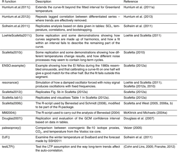
here. The details about the functions in replicationDemos are provided in Table 1, and when reference is made to Table 1 in the text below, it will serve as a description of which functions in the replicationDemos package that were used for a particular anal-ysis. More details about the methods are also given in the Appendix.

3 Replication demonstrations

15

3.1 Case 1: ignoring data which do not agree with the conclusions.

Humlum et al. (2011a) suggested that the moon and the giant planets in the solar system play a role a role in climate change on Earth, and that their influence is more important than changes in the GHG. A replication of their analysis can provide a means for turning these controversies into an educational exercise, and hence, provide a link

20

to agnotology.

The core of the analysis carried out by Humlum et al. (2011a) involved curve-fitting and tenuous physics, with a vague idea that the gravity of solar system objects

some-how can affect the Earth’s climate. The most severe problem with the paper, however,

1

(8)

ESDD

4, 451–505, 2013

Title Page

Tables Figures

◭ ◮

Back Close

Full Screen / Esc

Discussion

P

a

per

|

Dis

cussion

P

a

per

|

Discussion

P

a

per

|

Discussio

n

P

a

per

|

was that it had discarded a large fraction of data for the Holocene which did not fit their purports. Their reason for not showing the part of the data before 4000 BP was that

they “chose to focus on the most recent 4000 years of the GISP2 series, as the main

thrust of [their] investigation is on climatic variations in the recent past and their

poten-tial for forecasting the near future” (square brackets here denotes replacing “our” with

5

“their”). Humlum had also been a co-author on an older article in a popular technical magazine where this absent part of the data had been presented (Bye et al., 2011), and the data stretches almost 50 000 years back in time and is downloaded in one

single file2.

Humlum et al. (2011a) examined the last 4000 yr of the GISP2 (Greenland Ice Sheet

10

Project Two) record, and constructed a mathematical model based on a set of Fourier components and only three periods: 2804, 1186, and 556 yr (for Svalbard annual mean temperature since 1912, they found Fourier components of 68.4, 25.7, and 16.8 yr). Fourier series are often discussed in science textbooks and it is a mathematical fact that any finite series can be represented in terms of a series of sinusoids, which easily

15

can result in mere “curve-fitting” (Fourier expansion in this case). According to

Stephen-son (1973, p. 255), the sum of Fourier series is not necessarily equal to the functionf(x)

from which is derived, since the function given by the Fourier expansion is mathemati-cally bound to extend periodic regularity (known as the Dirichlet conditions). Moreover,

most functionsf(x), defined for a finite interval, are not periodic, although it is

possi-20

ble to find a Fourier series that represents this function in the given interval (Williams, 1960, p. 74). Pain (1983; p. 252) also clearly states that the Fourier series represent the

functionf(x) only within the chosen interval, and one can fit a series of observations

to arbitrary accuracy without having any predictability at all. This is a form of “over-fit” (Wilks, 1995), and therefore it is important to verify model to data outside the fitted

25

region.

2

(9)

ESDD

4, 451–505, 2013

Title Page

Tables Figures

◭ ◮

Back Close

Full Screen / Esc

Discussion

P

a

per

|

Dis

cussion

P

a

per

|

Discussion

P

a

per

|

Discussio

n

P

a

per

|

The underlying data used in (Humlum et al., 2011a) analysis violate the Dirichlet con-ditions, and their analysis is replicated here through replicationDemos. They claimed that they could “produce testable forecasts of future climate” by extending their statis-tical fit, and in fact, they did produce a testable forecast of the past climate by leaving out the period between the end of the last ice age and up to 4000 yr before present.

5

However, they did not state why the discarded data was not used for evaluation pur-poses, and the problem with their model becomes apparent once their fit is extended to the part of data that they left out.

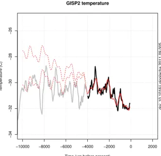
We extended their analysis back to the end of the last ice age. Figure 1 shows our replication of part of their results (Table 1). It clearly shows that the curve-fit for the

10

selected 4000 yr does not provide a good description for the rest of the Holocene. The

full red line shows their model results and the dashed red lines show two di_fferent

attempts to extend their model to older data. One initial attempt was made, keeping their trend; however this obviously caused a divergence. So in the second attempt, we removed the trend to give their model a better chance of making a good hindcast.

15

Again, the fit is no longer quite as good as presented in their paper. Clearly, their hypothesis of 3 dominant periodicities no longer works when extending the data period, and this is not surprising as this is explained in text books on Fourier methods.

In other words, the analysis made by Humlum et al. (2011a) was limited to a subset of the data, but they did not use the remaining part to evaluate their model. They

20

ignored the data which did not agree with their conclusions. Moreover, a lack of being universally valid suggests that the chosen method was not objective. Furthermore, they failed to acknowledge well-known shortcomings associated with curve-fitting, but rather based their analysis on unjustified fit to a set of Fourier series. Finally, their results lacked a well-formulated physical basis, and they failed to discuss past relevant

25

literature concerning the physics as well as mathematics.

(10)

ESDD

4, 451–505, 2013

Title Page

Tables Figures

◭ ◮

Back Close

Full Screen / Esc

Discussion

P

a

per

|

Dis

cussion

P

a

per

|

Discussion

P

a

per

|

Discussio

n

P

a

per

|

Scafetta (2012a, b, c) and Loehle and Scafetta (2011; henceforth “L&S2011”) fail to provide reliable answers.

3.2 Case 2: unclear physics and non-objective analytical design

Scafetta (2012a) too argued that celestial forcing in the form of gravitational forces from the giant gas planets explains most of the past climatic changes on Earth, and

5

especially fluctuations of ∼20 and ∼60 yr. He then evaluated how well global climate

models reproduce the amplitude and phase of∼20 and ∼60 yr periodicity, which he

attributed to the influence of gravity from celestial objects. In addition, he carried out an

evaluation of trends based on an arbitrary curve fitting, using di_fferent trend models for

different parts of the data, which apparently gave a good fit to the data. Although the

10

physics was vague, Scafetta argued that resonant response could amplify the weak

e_ffect from the planets, just like L&S2011. In addition to vague physics, many of the

statistics presented in the paper were miscalculated. By repeating the work done by Scafetta, we can understand why his purports diverge from the mainstream climate science. In this sense, this paper is a good agnotological example

15

Scafetta (2012a) can be reviewed in terms of the physics and the statistical analysis. The paper failed to acknowledge that resonance is an inherent property of a system, and will pick up any forcing with matching frequency. Our replications demonstrated that the paper presented an inappropriate analytical setup which favoured one outcome due to its design.

20

A weak forcing and a pronounced response would imply a positive feedback, or at least an optimal balance between forcing periodicity and damping rate (a 60 yr peri-odicity would suggest very weak damping, which seems unlikely, and hence the most convincing argument for resonance would involve a delayed positive feedback), and a preferred frequency would be an inherent characteristic of the earth climate system.

25

(11)

ESDD

4, 451–505, 2013

Title Page

Tables Figures

◭ ◮

Back Close

Full Screen / Esc

Discussion

P

a

per

|

Dis

cussion

P

a

per

|

Discussion

P

a

per

|

Discussio

n

P

a

per

|

if given a noisy forcing, even if the forcing itself has another dominant frequency (Ta-ble 1). Furthermore, a resonant system will respond to a trend in GHG forcings (in

mathematical terms, the forcing is proportional to ln|CO2|), and if such a resonance

implies positive feedbacks, these should also be present in a situation of GHG forc-ings. Hence it is extremely hard to attribute a cause for resonant response just from

5

analysing cycles when several forcings are present.

Another weakness in the analysis presented in Scafetta (2012a) is the handling of trends, as a quadratic trend that conveniently fitted the data was used for the

pe-riod 1850–2000, and then a linear fit with a warming rate of 0.009◦C yr−1 was used

after 2000. The quadratic equation for 1850–2000p(t)=4.9×10−5 x2–3.5×10−3x–

10

0.30 (Eq. 4, where x=t – 1850) gave a warming rate dp/dt=2 × 4.9 × 10−5x–

3.5×10−3₌0.011◦C yr−1for year 2000. Hence, the method used by Scafetta implicitly

assumed that the rate of warming was abruptly reduced in year 2000 for the future. It also implied that the future warming rate was smaller than the range reported in Solomon et al. (2007), and much of the recent warming was mis-attributed to natural

15

variations based on curve-fitting similar to that of Humlum et al. (2011a).

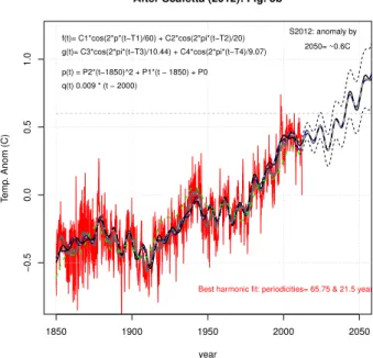
There seem to be a number of other results in Scafetta (2012a) which are difficult to

reproduce, as a replication of Fig. 5b in the paper (Table 1) suggests that it displays a lower projected trend than produced by the equations cited in the paper (Fig. 2). He also limited the confidence interval to one standard deviation (which implies a 68.6 %

20

confidence interval) in the evaluation to see whether the model results overlapped the observations (the more commonly used 95th confidence is roughly spanned by 2 times the error estimate). Other mistakes in the paper included a misapplication of the chi-squared test used to asses the global climate models (GCMs) against the ob-servations, where Scafetta used the squared error-estimates in the denominator;

con-25

ventional chi-squared tests do not square the denominator, see e.g. Wilks (1995) and Press et al. (1989).

The gravest issue with the Scafetta (2012a) analysis involved a series of tests which

(12)

ESDD

4, 451–505, 2013

Title Page

Tables Figures

◭ ◮

Back Close

Full Screen / Esc

Discussion

P

a

per

|

Dis

cussion

P

a

per

|

Discussion

P

a

per

|

Discussio

n

P

a

per

|

amplitude and phase of 20 and 60 yr oscillations in the global mean temperatures, assuming that these were due to the gravitational influence from celestial bodies. The phase and amplitudes found for the observations then were used as a yard stick for the GCM results, and a regression analysis was used where the covariates were the same as for the observations, with exactly the same phase and amplitude specified for the

5

20 and 60 yr oscillations. We know a priori that the planets are not accounted for in the CMIP3 climate simulations (Meehl et al., 2007), and hence Scafetta’s strategy is not suitable to provide an objective answer. A more appropriate null hypothesis would be that the amplitudes seen for the 20 and 60 yr variations would be due to noise. Hence, it is important to allow the phase to be unconstrained in the analysis, as we have

10

done (Fig. 3). When we repeat the analysis using a suitable setup, we do not see a falsification of the null-hypothesis, especially if we account for the fact that the analysis involves multiple tests and take the field significance into account (Wilks, 2006).

Scafetta (2012a) assumed that his method was validated if it was calibrated on one cycle of 60 yr and then was able to reproduce the next 60 yr cycle in the data that was

15

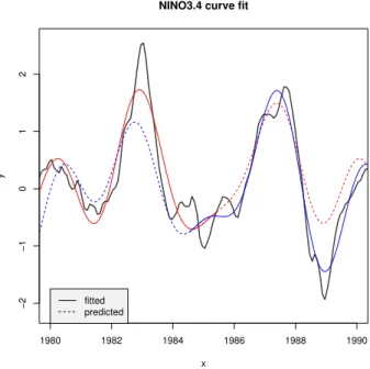
not part of the calibration. However, this argument is not justified, as this type of ap-proach fails for the El Ni ˜no Southern Oscillation (ENSO), for which it is well known that there were two El Ni ˜nos during the 1980s, which taken together, resemble two periods of a periodic cycle (Fig. 4). While each event provides a good fit for the other cycle, if calibration is performed on half of the decade and evaluated against the other, the

pre-20

dictions by this regression model fails to capture the variations outside this interval. It is therefore important to capture many cycles in a time series before one can establish a periodic signal, as only two cycles will likely not be representative of the entire system. In other words, the results in Scafetta (2012a) were incorrect due to inappropri-ate strinappropri-ategy for which the one answer was favoured, in addition to wrong statistics.

25

(13)

ESDD

4, 451–505, 2013

Title Page

Tables Figures

◭ ◮

Back Close

Full Screen / Esc

Discussion

P

a

per

|

Dis

cussion

P

a

per

|

Discussion

P

a

per

|

Discussio

n

P

a

per

|

4 Discussion and conclusions

More examples, listed in Table 1, are provided in the appendix. These involve issues

such as ignoring tests with negative outcomes, insufficient model evaluation, untested

presumed dependencies, misrepresentation of statistics, a failure to account for the actual degrees of freedom, lacking similarities, implausible physics, circular

reason-5

ing, incorrect interpretation of mathematical concepts, differences in data processing,

selective use of data, ignoring relevant scales, and contamination by external factors. Some common traits of unpersuasive papers may include speculations about cycles, and it is apparent from Table 2 that there are various claims which together involve a wide range of periodicities. Spectral methods tend to find cycles, whether they are real

10

or not, and it is no surprise that a number of periodicities appear when carrying out such analyses.

The merit of replication, by re-examining old publications in order to asses their ve-racity, is obvious. Published results in particular should be replicable, and access to open source codes and data should be regarded as a scientific virtue that facilitates

15

more reliable knowledge. Results are far more persuasive if one can reproduce them oneself, although replication of published results requires scientific training, numerical skill, and mastering of statistics. One concern is that modern research is veering away from the scientific virtue of replication and transparency. Open-source methodology of-ten does not belong to categories of articles in the scientific journals, and data is ofof-ten

20

inaccessible due to commercial interests and political reasons. Such limitations are

es-pecially unfortunate if the society at large has to make difficult choices depending on

nontransparent knowledge, information, and data. It is widely recognised that climate sciences have profound implications for society (Solomon et al., 2007), and that the communication of misleading claims is a case of agnotology. Furthermore, the

agno-25

(14)

ESDD

4, 451–505, 2013

Title Page

Tables Figures

◭ ◮

Back Close

Full Screen / Esc

Discussion

P

a

per

|

Dis

cussion

P

a

per

|

Discussion

P

a

per

|

Discussio

n

P

a

per

|

According to Sherwood (2011), unjustified claims and harsh debates are not new; history shows that they have been part of the scientific scene for a long time. Science is about trial and error, where errors and mistakes may be seen as an inevitable part of the process of learning, and may be valuable as a pedagogic tool to improve un-derstanding of the science (Bedford, 2010). Academic societies and institutions could

5

take a greater role in ensuring that the society gets the best information and knowl-edge that can be derived from science, by acting as trusted, respected, neutral and independent bodies replicating the results of high-profile papers or those influencing policy-makers, cited in the media and blogs. They could take science to the society (“domesticating science”), and show what kind of detective work lies behind the results.

10

Hence demonstrate how the conclusions are reached, based on the scientific virtues of transparency, replicability, testability, and objectivity. The interest in resolving con-tested issues by sharing analysis codes, however, has sometimes been low (Le Page, 2009), and the demonstrations provided here may serve as an example of how past work can be re-assessed (Pebesma et al., 2012). The IPCC could also have played

15

such a role; however, its target group has not been the general public, and critics argue that it has failed to correct the myths about climate research (Pearce, 2010). Another issue is that the source code used and data for producing the figures and tables in the IPCC’s assessment reports could be made openly available, in the same vein as the replicationDemos software and as proposed by Pebesma et al. (2012). There are

20

already some examples where there is free access to climate data (e.g. Lawrimore et al., 2013).

A1 Method – further details

All the data sets contained in replicationDemos are provided with the attribute “url” which identifies their data source on the Internet. The R-package contains examples

25

(15)

ESDD

4, 451–505, 2013

Title Page

Tables Figures

◭ ◮

Back Close

Full Screen / Esc

Discussion

P

a

per

|

Dis

cussion

P

a

per

|

Discussion

P

a

per

|

Discussio

n

P

a

per

|

The installation of the R-package can be done through a few command lines in R

(here the R-prompt “>” is shown) – start R and then write these lines in the R window:

> install.packages(“replicationDemos”)

> library(replicationDemos)

The installation of the R-package requires Internet access. Some of the functions also

5

read data directly over the Internet. Table 1 gives an overview of the cases which can be replicated through the replicationDemos package. Some of these may take some time if a large set of Monte-Carlo simulations is carried out. The replications should be

possible on different platforms (Linux, Mac, and Windows). The replications of case 1

can be implemented through typing the command line in R:

10

> Humlum.et.al.2011()

The source-code is produced with the following line (the name of the functions without the parentheses “()”):

> Humlum.et.al.2011

The manual page for the R-function replicating the predictions by Humlum et al. (2011)

15

are provided through:

> ?Humlum.et.al.2011

Likewise, cases 2–3 can be replicated and studied in further detail through the func-tions:

> LoehleScafetta2011()

20

> Scafetta2011()

User guides for R are freely available as PDF documents, e.g. from the CRAN site. The

(16)

ESDD

4, 451–505, 2013

Title Page

Tables Figures

◭ ◮

Back Close

Full Screen / Esc

Discussion

P

a

per

|

Dis

cussion

P

a

per

|

Discussion

P

a

per

|

Discussio

n

P

a

per

|

which provides an archive of up-to-date as well as a history of past version (older ver-sions of replicationDemos are already stored there). Although this archive is away from where the journal archives its papers, it ensures a wider visibility of the package among users of R. Any errors in the code may be fixed in new versions of the R-package that will be uploaded to the archive, however, the version control of the submitted

R-5

packages ensures traceability.

A2 Additional examples

Here an extended list of examples is provided, both which are included in the replica-tionDemos package and cases which do not need replication in order to assess. All of these relate to agnotology as they have been used to support arguments presented in

10

the media and on the Internet. Many of these have been compiled in reports such as the NIPCC (Idso and Singe, 2009) and several blogs.

A2.1 Case 3: unclear physics and misappropriate curve-fitting

Loehle and Scafetta (2011; L&S2011) purported that 20 and 60 yr natural cycles in the global mean temperature estimates were due to natural cycles which they explained in

15

terms of solar and astronomical influences. Furthermore, they claimed there was only a weak linear trend in the global mean temperature, and explained this in terms of a

slight negative feedback in the climate system to CO₂. At the same time, it is easy to

reproduce the analysis and demonstrate why the conclusions drawn by L&S2011 are at variance with most of the climate research community, which also makes this case

20

a good agnotological example.

The problem with the L&S2011 includes both a lack of clear physical basis and the analytical setup. L&S2011 assumed some kind of selective and potent resonance to

so-lar and astronomical forcing while a negative feedback was acting for CO₂. Resonance

is inherent to the system, and it is di_fficult to conceive what it would entail that di_ffered

25

(17)

ESDD

4, 451–505, 2013

Title Page

Tables Figures

◭ ◮

Back Close

Full Screen / Esc

Discussion

P

a

per

|

Dis

cussion

P

a

per

|

Discussion

P

a

per

|

Discussio

n

P

a

per

|

cycles were estimated from a mere 160 yr of data. In a complex and non-linear system such as Earth’s climate, such an exercise is prone to be non-robust and non-stationary. Furthermore, the analytical setup was not validated against independent data, and the skill of the model was not properly assessed.

L&S2011 assumed similar resonance as Scafetta (2012a), with the same

weak-5

nesses. Furthermore, the methods used in L&S2011 su_ffered from many of the similar

flaws as those in Humlum et al. (2011a), even though L&S2011 employed a diff

er-ent strategy for spectral analysis. The type of analysis in L&S2011 was repeated in Scafetta (2012a). Again, it is important to keep in mind that all curves (finite time series)

can be represented as a sum of sinusoids describing cycles with different frequencies

10

(Table 1). Furthermore, Fourier transforms are closely related to spectral analysis, but these concepts are not exactly the same. Spectral analysis also tries to account for mathematical artifacts, such as “spectral leakage” (Press et al., 1989), attribute proba-bilities that some frequencies are spurious, and estimate the significance of the results.

There is a number of di_fferent spectral analysis techniques, and some are more suitable

15

for certain types of data. Sometimes, one can also use regression to find the best-fit combination of sinusoids for a time series, as in L&S2011’s “empirical decomposition” (Table 1). It is typical, however, that geophysical time series, such as the global mean temperature, are not characterised by one or two frequencies. In fact, if we try to fit other sinusoids to the same data as L&S2011, we get many other frequencies which

20

fit equally well, and we see that the frequencies of 20 and 60 yr are not the most domi-nant ones. A trial with a range of periodicities for harmonic fitting in a similar regression analysis suggested that periodicities of 65.75 and 21.5 yr gave a better fit in terms of

value explained (R2) than 60 and 20 yr respectively (Table 1).

Fitting sinusoids with long time scales compared to the time series is careless, which

25

(18)

ESDD

4, 451–505, 2013

Title Page

Tables Figures

◭ ◮

Back Close

Full Screen / Esc

Discussion

P

a

per

|

Dis

cussion

P

a

per

|

Discussion

P

a

per

|

Discussio

n

P

a

per

|

that L&S2011 used to fit their model, and compare the fits for each segment (Table 1). The 20 and 60 yr amplitude estimates vary substantially from sequence to sequence when we adopt the same strategy as in L&S2011 (Table 1), and the amplitude for the fits to the shorter sequences will typically be 4 times greater than a similar fit gives for the original 10 000 yr long series. This is because there is a band of frequencies

5

present in random, noisy and chaotic data, which brings us back to our initial point: any

number or curve can be split into a multitude of different components, most of which

will not have any physical meaning.

The analysis presented in L&S2011 can be described as a curve-fitting exercise based on two periods and that assumed that cycles with constant frequency in a

non-10

linear and chaotic system. The paper also failed to provide a persuasive account of the physics behind the purported links.

A2.2 Case 4: ignoring negative tests

Solheim et al. (2011; SSH2011) argued that 60 % of the annual and winter temperature variations at Svalbard are related to the solar cycle length (SCL). The basis for their

15

conclusions was a high correlation estimated between SCL and the temperature esti-mates, and results from a Durbin-Watson test. The highest correlation reported were

−0.82 for the winter mean of the decade lagging one solar cycle. Repeating their

anal-ysis with our open-source agnotological toolkit gave different answers. The conclusions

from this paper has been disseminated by the organisation “klimarealistene”, who also

20

try to reach the Norwegian schools. In order to shed light on the agnotological aspects of this case, we need to replicate their work.

The conclusion of the paper lacked clear physical basis, as the chain of processes linking the solar cycle length and temperatures in the Arctic over the subsequent decade is not understood. Furthermore, the analysis was not objective, inflating the

25

(19)

ESDD

4, 451–505, 2013

Title Page

Tables Figures

◭ ◮

Back Close

Full Screen / Esc

Discussion

P

a

per

|

Dis

cussion

P

a

per

|

Discussion

P

a

per

|

Discussio

n

P

a

per

|

of the significance of the results. There is a good chance of seeing false fortuitous correlations if one examines enough local temperature records.

When we reconstructed their Table 1 we got nearly the same results, albeit not iden-tical. SSH2011 stated that they based their method for estimating SCL on a publication from 1939 (Waldmeier, 1961), however, more recent work on the estimation of SCL

5

account for uncertainties in estimating the true SCL as the sunspot record exhibits stochastic variations around the slow Schwabe cycle. Rather than estimating the SCL from the few data points around the solar minima, Benestad (2005) proposed to use a Fourier truncation to fit the sunspot record and hence use the entire data sample to estimate the SCL.

10

In particular, SSH2011’s estimate of the SCL for cycle 23 (12.2 yr) was substan-tially longer than the estimate of 10.5 yr reported by the Danish Meteorological Institute (based on Friis-Christensen and Lassen (1991) and follow-up studies) and 10.8 yr es-timated by Benestad (2005) (Table 1). Such a long cycle is the basis for their projected

cooling (a decrease from−11.2 to −17.2◦C with a 95 % confidence interval of−20.5

15

to−14◦C) at Svalbard over solar cycle 24 (starting 2008). The observed mean over

2008–2011 suggests a continued warming that reached −9.17◦C as an average for

the 4 yr, which means that the mean winter temperature of 2012–2018 (the next 7

win-ter seasons) must be−21.8◦C for a good prediction. An analysis of 7-season running

mean values of the Svalbard temperature reveals that it is rarely below−15◦C and has

20

never been as low as−21◦C since the measurements began.

SSH2011 used a weighted regression to account for errors of the mean temperature estimates over the periods corresponding to solar cycles. Hence they accounted for errors in the mean estimate, but neglected the errors associated with the SCL, which are more substantial than the errors in the mean seasonal or annual temperature over

25

10 yr segments. They also applied a bootstrapping approach to estimate the errors

in the correlation coe_fficients (between −0.52 and −0.97), as they argued that there

(20)

ESDD

4, 451–505, 2013

Title Page

Tables Figures

◭ ◮

Back Close

Full Screen / Esc

Discussion

P

a

per

|

Dis

cussion

P

a

per

|

Discussion

P

a

per

|

Discussio

n

P

a

per

|

a correlation for the winter of 0.37 with 95 % confidence interval between −0.39 and

0.83, and when using the previous cycle SCL, we got−0.84 with a confidence interval

between−0.39 and−0.96 (as opposed to−0.52 and−0.97 reported by SSH2011). The

“cor.test” test statistic is based on Pearson’s product moment correlation coefficient

“cor(x, y)” and follows a t-distribution with “length(x)-2” degrees of freedom, and an

5

asymptotic confidence interval is given based on Fisher’s Z transform. Hence, the claim made by SSH2011 that there is no analytical expression for estimating confidence intervals for correlation is false.

Their estimate of the errors in the correlation involved 1000 picks of random paired sub-samples from the SCL and temperatures, where the same pair sometimes were

10

picked more than once. A more appropriate strategy would be to carry out a set of

Monte-Carlo simulations accounting for the errors due to the SCL (η_S) and mean

temperature estimates (η_T). Here the symbol (subscripts) “S” refers to SCL and “T”

refers to the local winter mean temperature. We estimated the error in SCL from

the standard deviation of the di_fference between the SCL estimates from SSH2011

15

and Benestad (2005): η_S=σ_S, where σ_S is the standard deviation of the SCL

dif-ference: S_HSS2011–S_B2005. Then we re-calculated the 95 % confidence interval of the

correlation estimates by adding white noise to temperature and SCL with standard

de-viations ofσ_Sfor SCL, and for temperature we took the error of the mean estimate to

be σT/n1/2 where n is 10 for each 10 yr long segment. The Monte-Carlo simulation

20

of the correlations between temperature and SCL were then estimated as: cor(T+η_T,

S+η_S), and was repeated 30 000 times with different random realisations of the error

terms ηT and ηS (Table 1). The Monte-Carlo simulations gave a 95 % confidence

in-terval for the correlation between−0.85 to 0.08, substantially wider than both “cor.test”

and SSH2011. However, the latter two did not account for the uncertainties in the SCL

25

(21)

ESDD

4, 451–505, 2013

Title Page

Tables Figures

◭ ◮

Back Close

Full Screen / Esc

Discussion

P

a

per

|

Dis

cussion

P

a

per

|

Discussion

P

a

per

|

Discussio

n

P

a

per

|

The Monte-Carlo simulation also revealed that the SSH2011 correlation estimate was not centered in the simulated correlation error distribution, but was biased towards higher absolute values. The correlation estimate based on the Benestad (2005) SCL, on the other hand, gave a better match with the mean correlation from the Monte-Carlo simulation, although this too had a greater absolute value than the mean error

esti-5

mate. Furthermore, the bootstrapping approach adopted by SSH2011 seemed to give a biased error distribution, and we did not get the same 95 % confident limits as they did (we made 30 000 iterations). From just 9 data points, we find it quite incredible that the magnitude of their lower confidence limit was higher than 0.5. These results there-fore suggest that the choice made in SSH2011 of SCL was indeed “fortunate” within

10

the bounds of error estimates by getting correlations in the high end of the spectrum.

Since SSH2011 made at least 10 different tests (zero and one SCL lag and for 4

seasons plus the annual mean), the true significance can only be estimated by a field

significance test, e.g. the Walker test:p_W=1−(1−α_global)1/K (Wilks, 2006). The reason

is that from 100 random tests, about 5 % are expected to achieve scores that are at

15

the 5 % significance level. Another question is how many other temperature series that have been examined, as the appropriate number of tests to use in the Walker test should include all (also any unreported) tests in order to avoid a biased selection or lucky draw. When we estimate the p-value of their correlation from the null-hypothesis

derived from the Monte-Carlo simulations, we find that all the p-values exceedp_W, and

20

hence their results are not statistically significant at the 5 %-level.

Solheim et al. (2012) expanded the correlation exercises between SCL and tem-perature to include several locations in the North Atlantic region. The fact that several of these give similar results can be explained from the spatial correlation associated with temperature anomalies on time scales greater than one month. Their analysis

in-25

(22)

ESDD

4, 451–505, 2013

Title Page

Tables Figures

◭ ◮

Back Close

Full Screen / Esc

Discussion

P

a

per

|

Dis

cussion

P

a

per

|

Discussion

P

a

per

|

Discussio

n

P

a

per

|

and apply e.g. the Walker test. The failure to do so will give misleading results. The replication of SSH2011 is implemented with the following command lines in R:

> Solheim.et.al.2011()

The main problem with the analysis presented by SSH2011 was the lack of a

convinc-5

ing physical basis, inappropriate hypothesis testing, the inflation of significance, and a

small data sample insufficient to support the conclusions.

A2.3 Case 5: presumed dependencies and no model evaluation

Scafetta and West (2007, 2006a, b, 2005) argued that the recent increases in the global mean temperature were influenced by solar activity rather than increased GHG

10

concentrations.

The analysis, on which Scafetta and West based their conclusions, assumed that the global mean temperature was not influenced by factors other than solar variability on decadal to multi-decadal time scales. Furthermore, they dismissed the role of in-creased concentrations of GHG, based on the model fit to the solar trend, assuming

15

that a solar influence excludes the e_ffect from increased CO2-levels.

Scafetta and West assumed that all the climate variability over wide frequency bands spanning 11 and 22 yr were due to changes in the Sun. They developed a model which was not evaluated against independent data, and hence they had no information about its skill. Benestad and Schmidt (2009) demonstrated that the strategies employed in

20

Scafetta and West (2005, 2006a, b, 2007) were unsuitable for analysing solar-terrestrial relationships, and the source code for replicating these studies is included in replica-tionDemos (Table 1). Scafetta and West’s strategy failed to account for “spectral leak-age”, common trends, and the presence of a range of frequencies in chaotic signals. They applied a transfer function based on the ratio of the standard deviation for

respec-25

(23)

ESDD

4, 451–505, 2013

Title Page

Tables Figures

◭ ◮

Back Close

Full Screen / Esc

Discussion

P

a

per

|

Dis

cussion

P

a

per

|

Discussion

P

a

per

|

Discussio

n

P

a

per

|

filter (7.3–14.7 and 14.7–29.3 yr) to both. Moreover, their analysis a priori assumed that

no other factor was a_ffecting Earth’s climate over these wide ranges of time-scales, and

hence it is not surprising that they arrive at a misguided answer that seemed to suggest a strong solar influence.

The replication of the Scafetta and West papers, as done by Benestad and

5

Schmidt (2009), is implemented with the following command lines in R:

> Scafetta2006()

The Scafetta and West (2005, 2006a, b, 2007) papers demonstrate how potential mis-leading conclusions are drawn when the model has not been subject to careful

evalu-10

ation. Furthermore, their conclusions hinged on a set of assumptions which were not justified.

A2.4 Case 6: misinterpretation of statistics

Douglass et al. (2007) claimed that upper air trends predicted by global climate models were inconsistent with the trends measured by radiosondes and satellites. This

pur-15

ported discrepancy has been echoed on various Internet sites, been promoted by the

Norwegian organisation “klimarealistene”, and included in the NIPCC report. The flaw

in the analysis presented in this paper can easily be exposed through replication, and hence this is a perfect case in terms of agnotology.

The paper relied on an analysis which confused the confidence interval for the mean

20

estimate with the spread of a statistical sample, leading to a conclusion which was inconsistent with the results presented in the paper itself.

Douglass et al.’s (2007) conclusions were based on an inappropriate analytical set-up, and the flaw in their paper was caused by a confusion about the interpretation of

the error estimate±2σ_SE derived from the standard deviation σ of the di_fferent trend

25

(24)

ESDD

4, 451–505, 2013

Title Page

Tables Figures

◭ ◮

Back Close

Full Screen / Esc

Discussion

P

a

per

|

Dis

cussion

P

a

per

|

Discussion

P

a

per

|

Discussio

n

P

a

per

|

same notation as in the original paper, where the subscript “SE” denotes the error

estimate, andσ_SE=σ/(N-1)1/2, whereNis the sample (model ensemble) size.

Their invalid definition was taken to be the confidence interval of the data sample,

whereas the correct interpretation should the ∼95 % confidence interval for the

esti-mated mean value. The statistic that Douglass et al. (2007) wanted was an interval

5

describing the range of the data sample representing the trends predicted by climate models, in order to test whether the observed trends was distinguishable to any of the model results. To do so, the observations must be compared with the range of model results. However, the range of data samples cannot possibly decrease with increased

sample sizeN, which Douglass et al. (2007) implied when they used σ_SE to describe

10

confidence interval. On the other hand, the estimated mean value from a data sam-ple will become more accurate when estimated from a larger data samsam-ple, and the

confidence interval for this mean estimate is proportional toσ_SE.

In other words, Douglass et al. (2007) used the confidence interval for the mean value rather than for the sample and their test constituted an evaluation of how many

15

models were consistent with the mean of the ensemble. Hence, for some vertical lev-els their misconceived confidence limit excluded up to 59 % of the modlev-els from which it was derived (Table 1). Furthermore, if many more models with similar trend esti-mates had been added to the ensemble, the confidence interval for the mean value would diminish, however the spread would not necessarily be sensitive to the number

20

of models, and a larger sample would not imply that almost all the models fall outside the model spread. The replication of the Douglass et al. (2007) is implemented with the following command lines in R:

> Douglass2007()

25

(25)

ESDD

4, 451–505, 2013

Title Page

Tables Figures

◭ ◮

Back Close

Full Screen / Esc

Discussion

P

a

per

|

Dis

cussion

P

a

per

|

Discussion

P

a

per

|

Discussio

n

P

a

per

|

on the observations of the lower atmosphere also suggest even greater trends (Foster and Rahmstorf, 2011) and even better agreement between models and observations.

A2.5 Case 7: failure to account for the actual degrees of freedom

A paper by McKitrick and Michaels (2004a; MM2004) claimed that much of the histori-cal temperature trends could be explained from lohistori-cal economic activity, level of literacy,

5

and the heat island e_ffect. The analysis was based on a regression analysis between

local temperature trends and a set of economic co-variates.

MM2004 did not take into account the real degrees of freedom, as pointed out by Benestad (2004) who replicated their results. The economic co-variates would contain the same data within the border of each country, and temperature trends are smooth

10

functions in space. The analysis neither involved a proper validation of the regression model against independent data.

A simple test by splitting the data according to latitude and using one part for cal-ibration and the other for independent evaluation, demonstrated that the analysis of MM2004 was flawed (Table 1). Such a split-sample test had to make sure that there

15

were no dependencies between the samples used for calibration and evaluation, and

hence these samples would involve data from different regions.

A follow-up paper, McKitrick and Michaels (2007; MM07) involved similar flaws, re-vealed in Schmidt (2009) who concluded that the basis of their results was a set of correlations for a small selection of locations mainly from western Europe, Japan, and

20

the USA. Schmidt found that these projected strongly onto naturally occurring patterns of climate variability and their spatial auto-correlation implied reduced real degrees of freedom. Corresponding correlations from GCMs were found to vary widely due to the chaotic weather component in any short-term record, and the results of MM2007 did not fall outside the simulated distribution. There was therefore no evidence of any

25

(26)

ESDD

4, 451–505, 2013

Title Page

Tables Figures

◭ ◮

Back Close

Full Screen / Esc

Discussion

P

a

per

|

Dis

cussion

P

a

per

|

Discussion

P

a

per

|

Discussio

n

P

a

per

|

> MM2004()

MM2004 drew their conclusion based on inappropriate statistics, not recognising that the temperature trends vary slowly over space, and their regression analysis

misap-plied weights to the different covariates resulting in poor predictions of independent

5

data. Furthermore, recent studies indicates that the analysis for the ground tempera-tures is in accordance with the satellite-based analyses (Foster and Rahmstorf, 2011).

A2.6 Case 8: missing similarities

Veizer (2005) argued that galactic cosmic rays (GCR) are responsible for the most

re-cent warming. This conclusion assumes that the GCR affects cloudiness and hence the

10

planetary albedo, and provides a support for the purported dependencies by Svens-mark (1998) and Courtillot et al. (2007). The GCR have been introduced to the general society through popular science books (e.g. Svensmark, 2007) and videos (e.g. “The Cloud Mystery”), and have represented an important feature of agnotology in northern Europe. The influence of GHG has often been dismissed on grounds of the speculated

15

correlation between GCR and climate, assuming that the GCR-connection excludes

the effect of changes in the GHG concentrations.

Veizer (2005) failed to present any resemblance between the GCR-proxies discussed in the paper and a proxy for temperature, and he provided no quantitative statistical analysis on the correspondence between these quantities. Furthermore, the purported

20

dependency involved a neglect of the fact that many other factors may be more impor-tant in terms of generating cloud condensation nuclei.

The GCR are known to be modulated by solar activity through its influence on the inter-planetary magnetic field (IMF). In replicationDemos estimates based on Be-10 and temperature from the Vostoc ice cores can be shown together (Table 1), and any

25

(27)

ESDD

4, 451–505, 2013

Title Page

Tables Figures

◭ ◮

Back Close

Full Screen / Esc

Discussion

P

a

per

|

Dis

cussion

P

a

per

|

Discussion

P

a

per

|

Discussio

n

P

a

per

|

between Be-10 and the temperature proxy over the last 40 000 yr was−0.78 but this

number reflected the long time scales (greater than 5000 yr). The high frequency com-ponent was estimated by subtracting a low-pass filtered record, using a Gaussian win-dow with a width of 5000 yr. The correlation between the high-frequency components

were only−0.23 with a 95 % confidence interval of−0.65 to+0.30. The replication of

5

the Veizer (2005) is implemented with the following command lines in R:

> paleaoproxy()

In other words, it is di_fficult to discern any credible evidence linking GCR and recent

climate change, due to lacking correlation and the number of other factors present.

10

Veizer (2005) did not exclude other possibilities, but assumed that the other factors would be weak if there were a strong connection between GCR and climate.

A2.7 Case 9: looking at wrong scales

Humlum et al. (2013) argued that changes in CO₂follow changes in the temperature,

and that this implies that the increases seen in the Keeling curve are not man-made.

15

Their claims implicitly support the CO₂-curve presented by Beck (2008), and the meme

that the increase in the CO₂ concentrations seen in the Keeling curve is not due to

the burning of fossil fuels, has long been an aspect of agnotology surrounding the global warming issue. It is also acknowledged in Humlum et al. (2013) that their paper

had received inputs from “klimarealistene” and people with documented connections to

20

organisations such asThe Science & Environmental Policy Project (SEPP3) andThe

Heartland Institute4.

3

http://web.archive.org/web/20070215190653/http://www.sepp.org/Archive/NewSEPP/ ipccreview.htm

4