TEMA (São Carlos) vol.17 número3

(1)

Linear Algebra and Differential Calculus

in Pseudo-Intervals Vector Space

A. KENOUFI

Received on October 13, 2014 / Accepted on August 30, 2016

ABSTRACT.In this paper one proposes to use a new approach of interval arithmetic, the so-called pseudo-intervals [1, 5, 13]. It uses a construction which is more canonical and based on the semi-group completion into the group, and it allows to build a Banach vector space. This is achieved by embedding the vector space into free algebra of dimensions higher than 4. It permits to perform linear algebra and differential calculus with pseudo-intervals. Some numerical applications for interval matrix eigenmode calculation, inversion and function minimization are exhibited for simple examples.

Keywords:Pseudo-intervals arithmetic, free algebra, inclusion function, linear algebra, differential calcu-lus, optimization.

1 INTRODUCTION

Intervals are mathematical objects which allow to describe quantities with uncertainity due to the lack of knowledge of the studied phenomenon or experimental measurement accuracy. This is common in natural sciences and engineering. Even if nowadays we consider R.E. Moore [20, 21, 22, 29, 30] as the first mathematician who has proposed a rigorous framework for interval computations, the famous Archimedes from Syracuse (287-212 b.C) proposed 23 centuries be-fore a two-sides bounding ofπ: 3+10₇₁ < π <3+1₇.

Interval arithmetic, and interval analysis (IA) have been introduced as a computing framework which allows to perform analysis by computing mathematic bounds. Its extensions of the areas in applied and computational mathematics are important: non-linear problems, partial differential equations, inverse problems, global optimization and set inversion [1, 13, 14, 20, 21, 22, 30, 32]. It finds a large place of applications in controllability, automation, robotics, embedded systems, biomedical, haptic interfaces, form optimization, analysis of architecture plans, etc.

Several softwares and computational libraries to perform calculations with intervals such as

INTLAB[7], INTOPT90,GLOBSOL[12], and Numerica[27] have been developed those last

decades. But, due to the lack of distributivity ofIA, their Achille’s heel remains the construc-tion of the inclusion funcconstruc-tion from the natural one. Some approaches using boolean inclusion

(2)

tests, series or limited expansions of the natural function where the derivatives are computed at a certain point of the intervals, have been developed to circumvent this problem [1, 13, 14]. Nevertheless, those transfers from real functions to functions defined on intervals are not sys-tematic and not given by a formal process. This yields to the fact that the inclusion function definition has to be adapted to each problem with the risk to miss the primitive scope. Moreover, linear algebra and differential calculus need to be performed in the framework of vector space theory and not within semi-group one.

This article reminds first in Section 2 the definition and characteristics of the intervals semi-groupIR_{and the construction of its associated vector space}IR_{, and how to get an associative}

and distributive arithmetic of intervals, called pseudo-intervals arithmetic, by embedding the vector space into afree algebrawith dimension 4, 5, or 7 [1, 5, 13]. A systematic way to build inclusion functions, i.e. interval-valued functions defined onIR_{, is presented in Section 2. In}

Section 3, one shows thatIR_{can be endowed with a Banach space topology and allows}

differ-ential calculus. Since a new algorithm for set inversion within pseudo-intervals framework has already been presented in previous papers [1, 13], only examples of interval matrix eigenmode calculation, inversion, and minimization of interval functions are exhibited in each section. We have choosenpythonprogramming langage [28] to implement pseudo-intervals arithmetic. The main reason is that it is a free object-oriented langage, with a huge number of numerical libraries. Another advantage ofpythonis that first, it is possible to link the source code with others writ-ten in C/C++, FORTRAN, and second, it interacts easily with other calculations tools such as SAGE [31] and Maxima [19] in order to perform formal calculations. But here, one presents pure numerical applications inpython.

2 AN ALGEBRAIC APPROACH FOR INTERVALS

An interval X is defined as a non-empty, closed and connected set of real numbers. One writes real numbers as intervals with same bounds,∀a ∈ R ,a ≡ [a,a]. We denote by IR = P1

the set of intervals ofR_{. The arithmetic operations on intervals, called}_{Minkowski or classical}

operations, are defined such that the result of the corresponding operation on elements belonging to operand intervals belongs to the resulting interval. That is, if⋄ ∈ {+,−,∗, /}denotes one of the usual operations, one has, ifX and Y are bounded intervals ofR_,

X⋄Y = {x⋄y/x ∈X, y∈Y}, (2.1)

Although,IR_{is provided with a pseudo-inverse operation, it does not satisfy} X−X =0, and hence a substraction in the usual sense cannot be obtained. In many problems using interval arithmetic, that is the setIR_{with the Minkowski operations, there exists an informal transfers}

principle which allows, to associate with a real function f a function define on the set of intervals

IR_{which coincides with} f on the interval reduced to a point. But this transferred function is not unique. For example, if we consider the real function f(x)=x2+x=x(x+1), we associate naturally the functions f1, f2:IR−→IRgiven by f1(X)=X(X+1)and f2(X)=X2+X.

(3)

interesting transfers. But the qualitative “interesting” depends of the studied model and it is not given by a formal process.

In this paper, we determine a natural extensionIR_ofIR_{provided with a vector space structure.}

The vectorial substractionX Y does not correspond to the semantical difference of intervals and the intervalXhas no real interpretation. But these anti-intervals have a computational role.

An algebraic extension of the classical interval arithmetic, called generalized interval arith-metic [21, 32] has been proposed first by M. Warmus [33, 34]. It has been followed in the seventies by H.J. Ortolf and E. Kaucher [8, 9, 10, 11, 24]. In this former interval arithmetic, the intervals form a group with respect to addition and a complete lattice with respect to inclusion. In order to adapt it to semantic problems, Gardenes et al. have developed an approach called modal interval arithmetic [2, 3, 4]. S. Markov and others investigate the relation between general-ized intervals operations and Minkowski operations for classic intervals and propose the so-called directed interval arithmetic, in which Kaucher’s generalized intervals can be viewed as classic intervals plus direction, hence the name directed interval arithmetic [15, 16]. In this arithmetic framework, proper and improper intervals are considered as intervals with sign [17]. Interesting relations and developments for proper and improper intervals arithmetic and for applications can be found in literature [23, 26, 25].

Our approach [1, 5, 13], that we remind below in this article, is similar to the previous ones in the sense that intervals are extended to generalized intervals; intervals and anti-intervals correspond respectively to the proper and improper ones. However one uses a construction which is more canonical and based on the semi-group completion into a group, which allows then to build the associated real vector space, and to get an analogy with directed intervals.

2.1 The real vector spaceIR

LetIR_{be the set of intervals. It is in one to one correspondence and can be represented as a point}

in the half-plane ofR2_,_P₁_{= {}₍a,b)∈R2_,a ≤b}. The setP2= {(a,b)∈R2,a≥b}is the set

of anti-intervals.IR_{is closed for the addition and endowed with a regular semi-group structure.}

The multiplication∗is not globally defined.

We recall briefly the construction proposed by Markov [18] to define a structure of abelian group. As(IR_,₊₎_{is a commutative and regular semi-group, the quotient set, denoted by}IR_{, associated}

with the equivalence relations:

(A,B)∼(C,D)⇐⇒A+D=B+C,

for allA,B,C,D ∈IR_{, is provided with a structure of abelian group for the natural addition:}

(A,B)+(C,D)=(A+C,B+D)

where(A,B)is the equivalence class of(A,B). We denote by(A,B)the inverse of(A,B)

(4)

We have (A,B) =(B,A). If X = [a,a],a ∈ R_{, then}(X,0) = (0,−X)where−X = [−a,−a], and (X,0) = (0,X). In this case, we identifyX = [a,a]witha and we denote always byR_{the subset of intervals of type}[a,a].

Naturally, the group IR _{is isomorphic to the additive group} R2 _{by the isomorphism}

(([a,b],[c,d]) → (a −c,b−d). We find the notion of generalized interval and this yields immediately to the following result:

Proposition 1.LetX=(X,Y)∈IR, and l : IR−→Rwhich gives the interval length. Thus

1. If l(Y) <l(X), there is an unique A∈IR R such that X=(A,0),

2. If l(Y) >l(X), there is an unique A∈IR R such that X=(0,A)=(A,0),

3. If l(Y)=l(X), there is an unique A=α∈R such that X=(α,0)=(0,−α).

Any elementX =(A,0)withA ∈IR₋R_{is said positive and we write}_X_>_{0. Any element}

X = (0,A) with A ∈ IR−R _{is said negative and we write}_X _< _{0. We write} _X ≥ X′ if

XX′≥0. For example ifX andX′are positive,X≥X′⇐⇒l(X)≥l(X′). The elements

(α,0)withα∈R∗_{are neither positive nor negative.}

In [18], one defines on the abelian groupIR_{, a structure of quasi linear space. Our approach is a}

little bit different. We propose to construct a real vector space structure. We consider the external multiplication:

· :R×IR−→IR

defined, for allA∈IR_{, by}

α·(A,0)=(αA,0), α·(0,A)=(0, αA),

for allα >0. Ifα <0 we putβ = −α. So we put:

α·(A,0)=(0, βA), α·(0,A)=(βA,0).

We denoteαXinstead ofα·X. This operation satisfies

1. For anyα∈RandX∈IRwe have:

α(X)=(αX), (−α)X=(αX).

2. For allα, β∈R_{, and for all}X,X′∈IR_{, we have}

⎧ ⎪ ⎨ ⎪ ⎩

(5)

Theorem 1. The triplet(IR,+,·)is a real vector space and the vectorsX1 = ([0,1],0)and

X2=([1,1],0)ofIRdetermine a basis ofIR. SodimRIR=2.

Proof. We have the following decompositions:

([a,b],0) =(b−a)X1+aX2, (0,[c,d]) =(c−d)X1−cX2.

The linear map

ϕ :IR−→R2

defined by

ϕ( ([a,b],0) )=(b−a,a), ϕ( (0,[c,d]) )=(c−d,−c)

is a linear isomorphism andIR_{is canonically isomorphic to}R2_.

Definition 1.(IR,+,·)is called the vector space of pseudo-intervals.

2.2 A 4-dimensional free algebra associated withIR

Consider the following subset ofP1:

⎧ ⎪ ⎨ ⎪ ⎩

P1,1= {(a,b)∈P1,a≥0,b≥0}, P1,2= {(a,b)∈P1,a≤0,b≥0}, P1,3= {(a,b)∈P1,a≤0,b≤0}.

One observes that the semi-groupIR_{can be identified to}_P₁_,₁∪P1,2∪P1,3.Let us consider as

well the following vectors ofR2

⎧ ⎪ ⎪ ⎪ ⎨ ⎪ ⎪ ⎪ ⎩

e1=(1,1),

e2=(0,1),

e3=(−1,0),

e4=(−1,−1).

They correspond to the intervals[1,1],[0,1],[−1,0], and[−1,−1]. Any point ofP1,1∪P1,2∪ P1,3admits the decomposition

(a,b)=α1e1+α2e2+α3e3+α4e4

withαi ≥0. The dependance relations between the vectorsei are

e2=e3+e1

e4= −e1.

(6)

the free algebra of basis{e1,e2,e3,e4}whose products correspond to the Minkowski products.

The multiplication table is

e1 e2 e3 e4

e1 e1 e2 e3 e4

e2 e2 e2 e3 e3

e3 e3 e3 e2 e2

e4 e4 e3 e2 e1

Definition 2.This algebra is associative and its elements are called pseudo-intervals.

2.3 Pseudo-intervals product

Letϕ :IR−→A4the natural injective embedding,F ⊂A4the linear subspace generated by

{e1−e2+e3,e1+e4},ψthe canonical embedding fromA4toA4/Fandϕ′=ψ◦ϕ[1, 5, 13].

We identify an interval with its image inA4. The applicationϕis not bijective. Its image on the

elementsX=(X,0)=([a,b],0)is ⎧

⎪ ⎨ ⎪ ⎩

X= [a,b] ∈P1,1, ϕ(X)=ae1+(b−a)e2 (a ≥0,b−a ≥0) X= [a,b] ∈P1,2, ϕ(X)= −ae3+be2 (−a≥0,b≥0)

X= [a,b] ∈P1,3, ϕ(X)= −be4+(b−a)e3 (−b≥0,b−a≥0).

Theorem 2.The multiplication

X•Y=ϕ−1(ϕ′(X).ϕ′(Y))

is distributive with respect the addition.

Proof. Practically the multiplication of two intervals will so be made: let X,Y ∈ R_{. Thus}

X =αiei,Y =βiei withαi, βj ≥0 and we have the product

X•Y =ϕ−1(ϕ′(X).ϕ′(Y))

this product is well defined becauseϕ′₍_X_).ϕ′₍_Y₎_∈ _{I m}_ϕ_{. This product is distributive because}

X•(Y +Z) = ϕ−1(ϕ′(X).ϕ′(Y +Z))

= ϕ−1(ϕ′(X).(ϕ′(Y)+ϕ′(Z)) = ϕ−1(ϕ′(X).ϕ′(Y)+ϕ′(X).ϕ′(Z)) = X•Y +X•Z

Remark. We have

(7)

We shall be careful not to return inIR_{during the calculations as long as the result is not found.}

Otherwise we find the semantic problems of the distributivity.

We extend naturally the mapϕ:IR−→A4toIRby

ϕ(A,0)=ϕ(A) ϕ(0,A)= −ϕ(A)

for everyA∈IR_.

2.4 Pseudo-intervals division

Division between intervals can also be defined with solvingX ·Y = (1,0,0,0)inA4or in a

isomorphic algebraA′₄. InA4we consider the change of basis

⎧ ⎪ ⎨ ⎪ ⎩

e₁′ =e1−e2

e_i′ =ei,i =2,3

e₄′ =e4−e3.

This change of basis shows thatA4is isomorphic toA′₄

e1 e2 e3 e4

e1 e1 0 0 e4

e2 0 e2 e3 0

e3 0 e3 e2 0

e4 e4 0 0 e1

.

The unit ofA′₄is the vectore1+e2. This algebra is a direct sum of two ideals: A′4= I1+I2

whereI1is generated bye1ande4andI2is generated bye2ande3. It is not an integral domain,

that is, we have divisors of 0. For examplee1·e2=0.

Proposition 2. The multiplicative groupA∗₄of invertible elements ofA4is the set of elements

x=(x1,x2,x3,x4)such that

x4= ±x1,

x3= ±x2.

This means that the invertible intervals do not contain 0. If x∈A∗₄we have:

x−1= x1

x2₁−x2₄,

x2

x2₂−x2₃,

x3

x2₂−x₃2,

x4

x2₁−x₄2

.

2.5 Pseudo-intervals monotonicity property

Let us compute the product of pseudo-intervals using the product inA4and compare it with the

Minkowski product. LetX = [a,b]andY = [c,d]two intervals.

Lemma 1.If X and Y are not in the same pieceP1,i, then X•Y corresponds to the Minkowski

(8)

Proof. i) If X ∈ P1,1andY ∈ P1,2thenϕ(X) =(a,b−a,0,0)andϕ(Y) =(0,d,−c,0).

Thus

ϕ(X)ϕ(Y) = (ae1+(b−a)e2)(de2−ce3)

= bde2−cbe3

= (0,bd,−cb,0) = ϕ([cb,bd]).

ii) IfX ∈P1,1andY ∈P1,3thenϕ(X)=(a,b−a,0,0)andϕ(Y)=(0,0,d−c,−d). Thus

ϕ(X)ϕ(Y) = (ae1+(b−a)e2)((d −c)e3−de4)

= (ad−bc)e3−ade4

= (0,0,ad−cb,−ad) = ϕ([bc,ad]).

iii) IfX ∈P1,2andY ∈P1,3thenϕ(X)=(0,b,−a,0)andϕ(Y)=(0,0,d−c,−d). Thus

ϕ(X)ϕ(Y) = (be2−ae3)((d −c)e3−de4)

= ace2−bce3

= (0,ac,−cb,0) = ϕ([bc,ad]).

Lemma 2.If X an Y are both in the same pieceP1,1orP1,3, then the product X•Y corresponds to the Minkowski product.

The proof is analogous to the previous.

Let us assume that X = [a,b]andY = [c,d]belong toP1,2. Thusϕ(X) =(0,b,−a,0)and ϕ(Y)=(0,d,−c,0). We obtain

X Y =(be2−ae3)(de2−ce3)=(bd+ac)e2+(−bc−ad)e3.

Thus

[a,b][c,d] = [bc+ad,bd+ac].

This result is greater that all the possible results associated with the Minkowski product. How-ever, we have the following property:

Proposition 3.Monotony property: LetX1,X2∈IR. Then

X1⊂X2=⇒X1•Z⊂X2•Z for all Z∈IR.

ϕ(X1)≤ϕ(X2)=⇒ϕ(X1•Z)≤ϕ(X2•Z)

The order relation onA4that ones uses here is

⎧ ⎪ ⎪ ⎪ ⎪ ⎪ ⎨ ⎪ ⎪ ⎪ ⎪ ⎪ ⎩

(x1,x2,0,0)≤(y1,y2,0,0)⇐⇒y1≤x1 and x2≤y2, (x1,x2,0,0)≤(0,y2,y3,0)⇐⇒ x2≤y2,

(0,x2,x3,0)≤(0,y2,y3,0)⇐⇒x3≤y3 and x2≤y2, (0,0,x3,x4)≤(0,y2,y3,0)⇐⇒ x3≤y3,

(9)

Proof. Let us note that the second property is equivalent to the first. It is its translation in

A4. We can suppose thatX1 and X2 are intervals belonging moreover to P1,2: ϕ(X1) = (0,b,−a,0), ϕ(X2)=(0,d,−c,0). Ifϕ(Z)=(z1,z2,z3,z4), then

ϕ(X1•Z)=(0,bz1+bz2−az3−az4,−az1+bz3−az2+bz4,0), ϕ(X2•Z)=(0,d z1+d z2−cz3−cz4,−cz1+d z3−cz2+d z4,0).

Thus

ϕ(X1•Z)≤ϕ(X2•Z)⇐⇒

(b−d)(z1+z2)−(a−c)(z3−z4)≤0,

−(a−c)(z1+z2)+(b−d)(z3=z4)≤0.

But(b−d),−(a−c)≤0 and z2,z3≥0. This impliesϕ(X1•Z)≤ϕ(X2•Z).

2.6 The algebrasAnand a better result of the product

We can refine the product to become closer to Minkowski’s one. Consider the one dimensional extensionA4⊕Re5 =A5, wheree5is a vector corresponding to the interval[−1,1]ofP1,2.

The multiplication table ofA5is

e1 e2 e3 e4 e5

e1 e1 e2 e3 e4 e5

e2 e2 e2 e3 e3 e5

e3 e3 e3 e2 e2 e5

e4 e4 e3 e2 e1 e5

e5 e5 e5 e5 e5 e5

.

The pieceP1,2is writtenP1,2 =P1,2,1∪P1,2,1whereP1,2,1 = {[a,b],−a ≤b}andP1,2,2=

{[a,b],−a≥b}. IfX = [a,b] ∈P1,2,1andY = [c,d] ∈P1,2,2, thus

ϕ(X).ϕ(Y)=(0,b+a,0,0,−a).(0,0,−c−d,0,d)=(0,−(a+b)(c+d),0,0,a(c+d)+bd).

Thus we have

X•Y = [−bd−ac−ad,−bc].

Example. LetX = [−2,3]andY = [−4,2]. We haveX ∈P1,2,1andY ∈P1,2,2. The product

inA4gives

X•Y = [−16,14].

The product inA5gives

X•Y = [−12,10].

The Minkowski product is

(10)

Thus the product inA5is better than the product inA4with respect to the partial order. Let’s

go further. Considering a partition ofP1,2, we can define an extension ofA4of dimensionn,

the choice ofndepends on the approach wanted of the Minkowski product. For example, let us consider the vectore6corresponding to the interval[−1,1₂]. Thus the Minkowsky product gives e6·e6=e7wheree7corresponds to[−1₂,1]. This yields to the fact thatA6is not an associative

algebra but it is the case forA7whose table of multiplication is

e1 e2 e3 e4 e5 e6 e7

e1 e1 e2 e3 e4 e5 e6 e7

e2 e2 e2 e3 e3 e5 e6 e7

e3 e3 e3 e2 e2 e5 e7 e6

e4 e4 e3 e2 e1 e5 e7 e6

e5 e5 e5 e5 e5 e5 e5 e5

e6 e6 e6 e7 e7 e5 e7 e6

e7 e7 e7 e6 e6 e5 e6 e7

Example. Let X = [−2,3]andY = [−4,2]. The decomposition on the basis{e1, . . . ,e7}

with positive coefficients writes

X =e5+2e7, Y =2e6.

X•Y =(e5+2e7)(4e6)=4e5+8e6= [−12,8].

We obtain now the Minkowski product.

Remark 1.Pseudo-intervals division can be defined as well inA5andA7.

2.7 Inclusion functions

It is necessary for some problems to extend the definition of a function defined for real numbers

f :R→R_{to function defined for intervals}[f] :IR→IR_{such as}[f]([a,a])= f(a)for any

a∈R_{. It will be convenient to have the same formal expression for} f and[f]. Usually the lack of distributivity in Minkowski arithmetic does not give the possibility to get the same formal expres-sions. But with the pseudo-intervals arithmetic we have presented, there is no data dependency anymore and one can define easily inclusion functions from the natural one. For example, let’s extend to intervals the real functions f0(x)=x2−2x+1, f1(x)=(x−1)2, f2(x)=x(x−2)+1.

Usually, with the Minkwoski operations, the three expressions of this same function for the inter-valX = [3,4]are[f]0(X)= [2,11],[f]1(X)= [4,9]and[f]2(X)= [6,12]. Data dependancy

occurs when the variable appears more than once in the function expression. The deep reason of that is the lack of distributivity in Minkowski arithmetic. But within the arithmetic developed in

A4or higher dimension free algebras [5], this problem vanishes. For example: withX = [3,4]

and sinceX ∈P11,

(11)

Sincee1=(1,0,0,0),e2=(0,1,0,0)and with means of product table, one has

ϕ([f]0(X)) = (3e1+e2)2−2(3e1+e2)+1

= 9e2₁+2·3e1e2+e2₂−2·3e1−2e2+1

= 9e1+6e2+e2−6e1−2e2+e1=4e1+5e2

= ϕ([4,9]), (2.3)

ϕ([f]1(X)) = (3e1+e2−1)2

= (2e1+e2)2

= 4e2₁+4e1e2+e22

= 4e1+4e2+e2

= 4e1+5e2

= ϕ([4,9]), (2.4)

and

ϕ([f]2(X)) = (3e1+e2)·(3e1+e2−2)+1

= 9e1+3e1e2−6e1+3e1e2+e22−2e2+e1

= 4e1+3e2+3e2+e2−2e2

= 4e1+5e2

= ϕ([4,9]). (2.5)

Thus,[f]0(X)= [f]1(X)= [f]2(X)= [4,9]and the inclusion function is defined univoquely

regardless the way to write the original one.

On the other hand, the construction of the inclusion function depends on the type of problem one deals with. If one aims to perform set inversion for example, it has to be done in the semi-group

IR_{. But, the substraction is not defined in}IR_{. This problem can be circumvented by replacing}

it with an addition and a multiplication with the intervale4 = [−1,−1]. This maintains the

associativity and distributivity of arithmetic and permits to introduce a pseudo-substraction. For example: if f(x)=x2−x =x(x−1)for real numbers, one defines[f](X)=X2+e4·X. One

reminds the product[−1,−1] · [a,b]is equal to[−b,−a]. Due to the fact that the arithmetic is now associative and distributive, one does not have data dependency anymore and[f](X)=

X2+e4·X=X·(X+e4). The last term corresponds to the transfer ofx(x−1). Division can

be transferred to the semi-group in the same way by replacing 1_x =x−1withXe4_.

(12)

transferred to[f] : X ≡(X,0)→ \(X,0)≡ \X. This means that[a,b]substraction is the anti-interval[−a,−b]addition. One of the most important consequence is that it is possible to transfer some functions directly to the pseudo-intervals. For example, it is easy to prove analytically in

IR_that[exp](([a,b],0))=([exp(a),exp(b)],0)with means of Taylor expansion.

2.8 Numerical linear algebra examples

One uses theA7pseudo-intervals arithmetic for simple examples of linear algebra computations

where matrix elements are intervals.

2.8.1 Interval matrix diagonalization

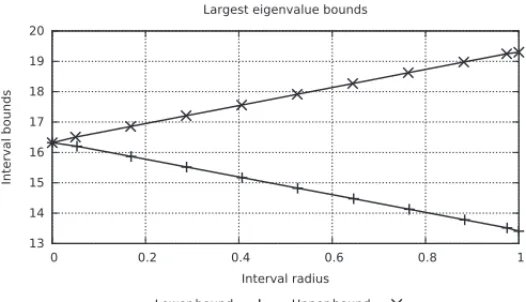
As an example, we would like to compute the largest eigenmode of the matrixMwhose elements are intervals centered around a certain real number with a radiusǫ:

M =

⎛ ⎜ ⎝

[2−ǫ,2+ǫ] [6−ǫ,6+ǫ] [5−ǫ,5+ǫ] [6−ǫ,6+ǫ] [2−ǫ,2+ǫ] [8−ǫ,8+ǫ] [5−ǫ,5+ǫ] [8−ǫ,8+ǫ] [6−ǫ,6+ǫ]

⎞ ⎟ ⎠.

If one usesscilabto compute the spectrum of the previous matrix without radius (ǫ =0), the highest eigenvalue is approximatively 16.345903 and the corresponding eigenvector is

(0.4728057,0.5716783,0.6705510). In order to show that arithmetics and interval algebra de-veloped above are robust and stable, let’s try to compute the highest eigenvalue of an interval matrix. One uses here the iterate power method, which is very simple and constitute the basis of several powerful methods such as deflation and others.

The Figures 1 and 2 show clearly for different value ofǫ the stability of the multiplication, and the largest eigenmode is recovered whenǫ = 0. The other eigen modes can be computed with the deflation methods for example which consists to withdraw the direction spanned by the eigenvector associated to the highest eigenvalue to the matrix by constructing its projector and to do the same. Several methods are available and efficient to achieve that [6, 35]. We have choosen to compute only the highest eigenvalue and its corresponding eigenvector in order to show simply the efficiency of our new arithmetic.

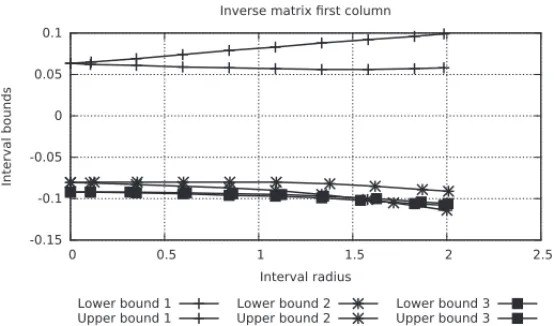
2.8.2 Interval matrix inversion

Let’s define the matrix X whose elements are intervals centered around a certain real number with a radiusǫ:

X =

⎛ ⎜ ⎝

[−2−ǫ,−2+ǫ] [−7−ǫ,7+ǫ] [4−ǫ,4+ǫ] [5−ǫ,5+ǫ] [−1−ǫ,−1+ǫ] [6−ǫ,6+ǫ] [9−ǫ,9+ǫ] [−8−ǫ,−8+ǫ] [3−ǫ,3+ǫ]

(13)

13 14 15 16 17 18 19 20

0 0.2 0.4 0.6 0.8 1

Interval bounds

Interval radius Largest eigenvalue bounds

Lower bound Upper bound

Figure 1: Largest eigenvalue convergence computed with iterate power method to the value computed withscilab16.345903.

0.45 0.5 0.55 0.6 0.65 0.7

0 0.1 0.2 0.3 0.4 0.5 0.6 0.7 0.8 0.9 1

Interval bounds

Interval radius

Component bounds of the eigenvector associated to the largest eigenvalue

Lower bound 1 Upper bound 1

Figure 2: Eigenvector components associated to the largest eigenvalue convergence computed with iterate power method to the eigenvector computed with scilab (0.4728057, 0.5716783, 0.6705510).

Scilabinversion function gives numerically forǫ=0

X−1=

⎛ ⎜ ⎝

−0.0924025 0.0225873 0.0780287 −0.0800821 0.0862423 −0.0657084 0.0636550 0.1622177 −0.0759754

⎞ ⎟

⎠. (2.6)

We would like to use the well-known Schutz-Hotelling algorithm [6, 35] to inverse the matrixX

since it uses simple arithmetic operations:

X0=

Xt

i,j A2i j

, Xj =Xj−1(2−A·Xj−1), ∀n ≥1 (2.7)

(14)

-0.15 -0.1 -0.05 0 0.05 0.1

0 0.5 1 1.5 2 2.5

Interval bounds

Interval radius Inverse matrix rst column

Figure 3: First column elements bounds convergence according interval radiusǫ.

0.02 0.04 0.06 0.08 0.1 0.12 0.14 0.16 0.18 0.2 0.22

0 0.2 0.4 0.6 0.8 1 1.2 1.4 1.6 1.8 2

Interval bounds

Interval radius Inverse matrix secund column

Figure 4: Second column elements bounds convergence according interval radiusǫ.

-0.1 -0.08 -0.06 -0.04 -0.02 0 0.02 0.04 0.06 0.08 0.1

0 0.2 0.4 0.6 0.8 1 1.2 1.4 1.6 1.8 2

Interval bounds

Interval radius Inverse matrix third column

(15)

3 TOPOLOGY OFIR

One shows in this section thatIR_{can be endowed with the metric topology of a Banach space.}

This permits to define correctly continuity and differentiability of functions.

3.1 Banach space structure ofIR

Any elementX ∈ IR _{is written}(A,0)or(0,A). We define its lengthl(X)as the length of A

and its center asc(A)or−c(A)in the second case.

Theorem 3.The map|| || :IR−→R+given by

||X|| =l(X)+ |c(X)|

for anyX∈IRis a norm.

Proof. We have to verify the following axioms: ⎧

⎪ ⎨ ⎪ ⎩

1) ||X|| =0⇐⇒X=0,

2) ∀λ∈R||λX|| = |λ|||X||,

3) ||X+X′|| ≤ ||X|| + ||X′||.

1) If||X|| =0, thenl(X)= |c(X)| =0 andX=0.

2) Letλ∈R_{. We have}

||λX|| =l(λX)+ |c(λX)| = |λ| ·l(X)+ |λ| · |c(X)| = |λ| · ||X||.

3) One considers thatI refers toXandJrefers toX′thusX=(I,0)or=(0,I). We have to study the two different cases:

i) IfX+X′=(I+J,0)or(0,I+J), then

||X+X′|| = l(I+J)+ |c(I+J)|

= l(I)+l(J)+ |c(I)+c(J)|

≤ l(I)+ |c(I)| +l(J)+ |c(J)|

= ||X|| + ||X′||.

ii) LetX+X′=(I,J). If(I,J)=(K,0)thenK +J =Iand

||X+X′|| = ||(K,0)||

= l(K)+ |c(K)|

(16)

that is

||X+X′|| ≤ l(I)+ |c(I)| −l(J)+ |c(J)|

≤ l(I)+ |c(I)| +l(J)+ |c(J)|

= ||X|| + ||X′||.

So we have a norm onIR_.

Theorem 4.The normed vector spaceIRis a Banach space.

Proof. In fact, all the norms onR2_{are equivalent and}R2_{is a Banach space for any norm. The}

vector spaceIR_{is then isomorphic to}R2_{. Thus, it is complete.}

Remarks.

1. To define the topology of the normed spaceIR_{, it is sufficient to describe the}ε -neighbor-hood of any pointχ0 ∈ IRforεa positive infinitesimal number. We can give a

geomet-rical representation, consideringχ0 = ([a,b],0)represented by the point(a,b) ∈ R2.

We assume thatχ0 = ([a,b],0)andεan infinitesimal real number. Let A1, . . . ,A4the

pointsA1=(a−ε,b−ε),A2 =(a+ε₂,b−₂ε),A3=(a+ε,b+ε),A4=(a−ε₂,b+ε₂).

If 0<a <b, then theε-neighborhood ofχ0 =([a,b],0)is represented by the

parallelo-grams whose vertices areA1,A2,A3,A4.

2. We can consider another equivalent norms onIR_{. For example}

||X|| = ||_X|| =max{|x|,|y|}

whereX=([x,y],0), but the initial one has a better geometrical interpretation.

3.2 Continuity and differentiability inIR

As IR _{is a Banach space, we can describe a notion of differential function on it. Consider}

X0=(X0,0)inIR. The norm||.||defines a topology onIRwhose a basis of neighborhoods is

given by the ballsB(X0, ε) = {X ∈IR,||XX0||< ε}. Let us characterize the elements of B(X0, ε).X0=(X0,0)=([a,b],0).

Proposition 4. ConsiderX0 = (X0,0) = ([a,b],0)in IR andε ≃ 0,ε > 0. Then every

element ofB(X0, ε)is of typeX=(X,0)and satisfies

l(X)∈ B_R(l(X0), ε1) and c(X)∈ BR(c(X0), ε2)

withε1, ε2≥0andε1+ε2≤ε, where BR(x,a)is the canonical open ball inRof center x and

(17)

Proof. First case:Assume thatX=(X,0)=([x,y],0). We have

XX0 = (X,X0)=([x,y],[a,b])

=

([x−a,y−b],0) if l(X)≥l(X0) (0,[a−x,b−y]) if l(X)≤l(X0)

Ifl(X)≥l(X0)we have

||XX0|| = (y−b)−(x−a)+

y−b+x−a

2 = l(X)−l(X0)+ |c(X)−c(X0)|.

Asl(X)−l(X0) ≥ 0 and |c(X)−c(X0)| ≥ 0, each one of this term if less thanε. If l(X)≤l(X0)we have

||XX0|| =l(X0)−l(X)+ |c(X0)−c(X)|.

and we have the same result.

Second case:ConsiderX=(0,X)=([x,y],0). We have

XX0=(0,X0+X)=([x+a,y+b])

and

||XX0|| =l(X0)+l(X)+ |c(X0)+c(X)|.

In this case, we cannot have||XX0||< εthusX ∈/B(X0, ε).

Definition 3.A function f :IR−→IRis continuous atX0if

∀ε >0,∃η >0 such that ||XX0||< η implies ||f(X) f(X0)||< ε.

Consider(X1,X2)the basis ofIRgiven in Section 2. We have

f(X)= f1(X)X1+ f2(X)X2 with fi :IR−→R.

If f is continuous atX0so

f(X) f(X0)=(f1(X)− f1(X0))X1+(f2(X)− f2(X0))X2.

To simplify notations letα= f1(X)−f1(X0)andβ=f2(X)−f2(X0). If||f(X)f(X0)||< ε,

and if we assume f1(X)− f1(X0) >0 and f2(X)− f2(X0) >0 (other cases are similar), then

we have

l(αX1+βX2)=l([β, α+β],0) < ε

thus f1(X)− f1(X0) < ε. Similarly,

c(αX1+βX2)=c([β, α+β],0)=

α

(18)

and this implies that f2(X)− f2(X0) < ε.

Corollary 1. f is continuous atX0if and only if f1and f2are continuous atX0.

Definition 4.ConsiderX0inIRand f :IR−→IRcontinuous. We say that f is differentiable

atX0if there exists a linear function g:IR−→IRsuch that

||f(X) f(X0)g(XX0)|| =o(||XX0||).

Examples.

• f(X) =X. This function is continuous and differentiable at any point. Its derivative is

f′(X)=1.

• f(X)=X2. ConsiderX0=(X0,0)=([a,b],0)andX∈B(X0, ε). We have

||X2_X2

0|| = ||(XX0)(X+X0)||

≤ ||XX0|| ||X+X0||.

Givenε >0, letη= ε ||X+X0||

, thus if||X_X₀_||_{< η}_{, we have}_||_X2_X2

0||< εand

f is continuous and differentiable. It is easy to prove that f′(X)=2Xis its derivative.

• Consider P = a0+a1X + · · · +anXn ∈ R[X]. We define f : IR −→ IR with

f(X) = a0X2+a1X+ · · · +annXn whereXn = X ·Xn−1. From the previous

ex-ample, all monomials are continuous and differentiable, it implies that f is continuous and differentiable as well.

• Consider the functionQ2given by Q2([x,y]) = [x2,y2]if|x| < |y| andQ2([x,y] =

[y2,x2]in the other case. This function is not differentiable.

3.3 Minimization examples

One uses theA7 pseudo-intervals arithmetic for simple examples of inclusion function

mini-mization with first and second order methods such as respectively fixed-step gradient descent and Newton-Raphson ones.

3.3.1 Fixed-step gradient descent method

(19)

-3.5 -3 -2.5 -2 -1.5 -1 -0.5 0 0.5 1

1 10 100 1000

Interval bounds

Iterations

Fixed step descent method with nite dierences

Figure 6: Convergence of the fixed-step gradient algorithm for the functionx −→x·exp(x)to an interval centered around[−1,−1] = −1.

-8 -6 -4 -2 0 2 4 6

1 10 100 1000

Gradient bounds

Iterations

Figure 7: Convergence of the fixed-step gradient algorithm for the derivative of the function

x−→x·exp(x)to an interval centered around[0,0] =0.

3.3.2 Newton-Raphson method

Let’s optimize the same functionx −→ x ·exp(x)with a second order method such as the Newton-Raphson one, which is the basis of all second order methods such as Newton or quasi-Newton’s ones [35]. One sets initial guess interval to[0,10], finite difference step to 10−3and accuracy of gradient to 10−9. One can state on Figures (8,9) that it finds the same minimum which is an interval centered around−1.

4 CONCLUSION

(20)

-2 0 2 4 6 8 10

1 10 100 1000

Interval bounds

Iterations

Figure 8: Convergence of the Newton-Raphson algorithm for the functionx −→ x·exp(x)to an interval centered around[−1,−1] = −1.

1e-06 0.0001 0.01 1 100 10000 1e+06

1 10 100 1000 10000

Gradient bounds

Iterations

Figure 9: Convergence of the Newton-Raphson algorithm for the derivative of the function

x−→x·exp(x)to an interval centered around[0,0] =0.

(21)

5 ACKNOWLEDGEMENTS

The author thanks Michel Gondran for useful and interesting discussions.

RESUMO.Neste artigo é proposto o uso de uma nova abordagem de aritmética intervalar, os chamados pseudo-intervalos [1, 5, 13]. Essa abordagem utiliza uma construção que é mais canônica e baseada na completude de semi-grupos em um grupo, e permite a construção de espaços vetoriais de Banach. Isso é alcançado através da imersão do espaço vetorial em uma álgebra livre de dimensão maior que 4. Desta forma é poss´ıvel realizar álgebra linear e cálculo diferencial com pseudo-intervalos. Algumas aplicações numéricas para o cálculo do espectro de matrizes intervalares, inversão e minimização de funções são mostradas como exemplos.

Palavras-chave: Aritmética pseudo-intervalar, álgebra livre, inclusão de funções, álgebra linear, cálculo diferencial, otimização.

REFERENCES

[1] B. Durand, A. Kenoufi & J.F. Osselin. System adjustments for targeted performances combining symbolic regression and set inversion.Inverse problems for science and engineering, (2013).

[2] A. Trepat, E. Gardenes & H. Mielgo. Modal intervals: Reason and ground semantics.Lecture Notes in Computer Science, Springer-Verlag, Berlin, Heidelberg,212(1986), 27–35.

[3] L. Jorba, R. Calm, R. Estela, H. Mielgo, A. Trepat, E. Gardenes & M.A. Sainz. Modal intervals. Reliable Computing,7(2001), 77–111.

[4] E. Gardenes. Fundamentals of sigla, an interval computing system over the completed set of intervals. Computing,24(1980), 161–179.

[5] N. Goze.PhD thesis, n-ary algebras and interval arithmetics. University of Haute-Alsace, (2011).

[6] A.S. Householder.The theory of matrices in numerical analysis. Dover Publications, (1975).

[7] http://www.ti3.tu-harburg.de/rump/intlab/.

[8] E. Kaucher.Ueber metrische und algebraische Eigenschaften einiger beim numerischen Rechnen auftretender Raume. Dissertation, Universitaet Karlsruhe, (1973).

[9] E. Kaucher. Algebraische erweiterungen der intervallrechnung unter erhaltung der ordnungs und ver-bandstrukturen computing.1(1977), 65–79.

[10] E. Kaucher. Ueber eigenschaften und en der anwendungsmoeglichkeiten der erweiterten intervall-rechnung und des hyperbolischen fastkoerpers ueber r computing.1(1977), 81–94.

[11] E. Kaucher. Interval analysis in the extended interval space ir computing.2(1980), 33–49.

[12] R.B. Kearfott.Rigorous Global Search: Continuous Problems. Academic Publishers, (1996).

[13] A. Kenoufi. Probabilist set inversion using pseudo-intervals arithmetic.Trends in Applied and Com-putational Mathematics,15(1) (2014), 97–117.

(22)

[15] S.M. Markov. Extended interval arithmetic involving infinite intervals.Mathematica Balkanica, New Series,6(3) (1992), 269–304.

[16] S.M. Markov. On directed interval arithmetic and its applications.J. UCS,1(7) (1995), 510–521.

[17] S.M. Markov.On the Foundations of Interval Arithmetic. Scientific Computing and Validated Numer-ics Akademie Verlag, Berlin, (1996).

[18] M. Markov. Isomorphic embeddings of abstract interval systems.Reliable Computing, (3) (1997), 199–207.

[19] http://maxima.sourceforge.net.

[20] R.E. Moore.PhD thesis. Standford university, (1962).

[21] R.E. Moore.Interval analysis. Prentice Hall, Englewood Cliffs, NJ, (1966).

[22] R.E. Moore. A test for existence of solutions to nonlinear systems. SIAM J. Numer. Anal., 14(4) (1977), 611–615.

[23] E. Popova, N. Dimitrova & S.M. Markov.Extended Interval arithmetic: New Results and Applica-tions. Computer Arithmetic and Enclosure Methods. Elsevier Sci. Publishers B.V., (1992).

[24] H.J. Ortolf. Eine verallgemeinerung der intervallarithmetik. geselschaft fuer mathematik und daten-verarbeitung.Bonn,11(1969), 1–71.

[25] E.D. Popova. All about generalized interval distributive relations. i. complete proof of the relations. Sofia, (2000).

[26] E.D. Popova. Multiplication distributivity of proper and improper intervals. Reliable Computing, 7(2) (2001), 129–140.

[27] Yves Deville, Pascal Van Hentenryck & Laurent Michel.Numerica: A Modelling Language for Global Optimization.MIT Press, (1997).

[28] http://www.python.org.

[29] C.T. Yang & R.E. Moore. Interval analysis i.LMSD-285875, Lockheed Aircraft Corporation, Missiles and Space Division, Sunnyvale, California, (1959).

[30] Wayman Strother, R.E. Moore & C.T. Yang. Interval integrals. LMSD-703073, Lockheed Aircraft Corporation, Missiles and Space Division, Sunnyvale, California,IX(4) (1960), 241–245.

[31] http://www.sagemath.org.

[32] T. Sunaga.Theory of an interval Algebra and its Application to Numerical Analysis.Number 2. RAAG Memoirs, (1958).

[33] Mieczyslaw Warmus. Calculus of approximations.Bull. Acad. Pol. Sci., C1, III(IV (5)) (1956), 253– 259.

[34] Mieczyslaw Warmus. Approximations and inequalities in the calculus of approximations. classifica-tion of approximate numbers.Bull. Acad. Pol. Sci. math. astr. & phys.,IX(4) (1961), 241–245.