Dispersionless Limit of Integrable Models
J. C. Brunelli
UniversidadeFederaldeSantaCatarina
DepartamentodeFsia{CFM
CampusUniversitario{Trindade
C.P.476, CEP88040-900
Florianopolis,SC{Brazil
brunellifs.ufs.br
Reeived7January,2000
Nonlineardispersionlessequationsariseasthedispersionlesslimitofwellknowintegrablehierarhies
ofequationsorbyonstrution,suhasthesystemofhydrodynamitype. Someoftheseequations
are integrable inthe Hamiltonian senseand appear in the studyof topologial minimalmodels.
Inthe rst part of the review, we will give abrief introdution to integrable models, mainly its
Laxrepresentation. Then,we willintroduethedispersionless limitandshowsomeofourresults
onerningthetwo-omponenthyperbolisystemofequationssuhasthepolytropigasand
Born-Infeldequations.
I Introdution
The study of integrable models or solvable
nonlin-ear partial dierential equations is an ative area of
researh sine the disovery of the inverse
satter-ing method [1-3℄. These models are in a sense
uni-versal sine they show up in many areas of physis
suh as solid state, nonlinear optis,
hydrodynam-is, eld theory just to name a few. Also,
inte-grablemodelsarelinkedtomanyareasofmathematis
(seethehartinhttp://www.ma.hw.a.uk/solitons/pros/
bullough1/bullough1/bullough1.html) andhavebeautiful
struturesbehindthem.
Inthisreview wewanttoapproahthe
dispersion-lesslimitofsomeintegrablemodelsanddesribesome
of our work on this subjet [4-7℄. This review is
or-ganized asfollows: In Setion II wereview or at least
introdue some basi fats on integrable models. We
usetheKorteweg-deVriesequation(KdV)asan
exam-ple. InSetionIIIweintroduethedispersionlesslimit
of anintegrablemodel using theKdV equationto
ob-tain theorrespondingRiemann equation. Setion IV
reviews ourwork witha speial lass of dispersionless
systems known as two-omponenthyperbolisystems.
WeshowourresultsonerningtheHamiltonian
stru-tures for the Riemann equation [4℄ the dispersionless
Laxrepresentationfor thepolytropigasdynamis [5℄
and Born-Infeldequation[6℄. Finally,in SetionV, we
onlude with some problems that deserve further
in-vestigations.
II Integrable Models
II.1 Solitons
We are interested in nonlinear partial dierential
equations suh as the sine-Gordon equation,
nonlin-earShrodinger equation, Korteweg-deVries equation
(KdV),et. These equations, aswewill see, are very
speialsinetheyareintegrable. Fromnowonwewill
illustrate themain results onerningintegrability
us-ingtheKdVequation.
The KdV equation has as solution what is alled
today a soliton. We an trae the disovery of
the soliton bak to 1834 with the Sott Russell's
experiment [8℄ to generate solitary waves in water,
i.e., loalized single entity waves. A modern
ver-sion of his experiment is shown in Fig. 1 (see
http://www.ma.hw.a.uk/hris/sott russel.html for an
attempttorereateSottRussell'ssoliton). Sott
Rus-sellfoundthat thevolumeV ofwaterwaveisequalto
thevolume ofwaterdisplaedand that thespeed of
thesolitarywaveisrelatedwithitsamplitudea,depth
ofwaterhandaelerationofgravityg by
2
=g(h+a) (1)
Thisequationshowsthathigherwavestravelfaster.
At-temptstoobtain(1)theoretiallyweredoneby
Boussi-nesq(1871)andLordRayleigh(1876)butanequation
foru(x;t) in thesmall amplitude (h a) and in the
u
t =uu
x +u
xxx
(2)
where u(x;t) is the wave prole and u
t =
u
t , u
x =
u
x ;:::.
Figure1. Generationofasolitarywave.
Theinterestinthe KdVequation(2) wasresumed
after studies of Fermi, Pasta and Ulam in 1955 [10℄
onnumerialmodelsofphonons in non-linearlatties,
whih are models losely related with the
disretisa-tionof theKdVequation. Motivated bythese results,
Zabusky andKruskalin 1965 [11℄ studied numerially
equations like (2) with periodi boundary onditions
and were led to introdue theonept of\soliton"
so-lutions. In1967 Gardner,Greene, Kruskaland Miura
[12℄ solved equation (2) exatly, introduing the
\In-verseSatteringTransformMethod"(ISTM),andwere
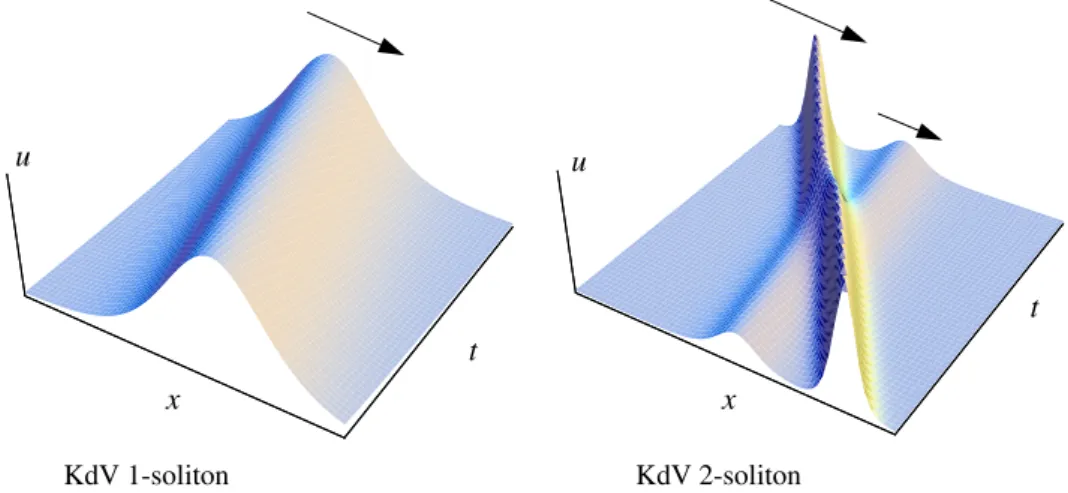
abletoobtainitsanalytiexpression. Thesoalled
1-solitonand2-solitonsolutionsoftheKdVequation(2),
forrapidlydereasingboundaryonditions
u(x;t)!0 for x!1;
are
u(x;t)= 1
2
2
seh 2
1
2 (x+
2
t)
! 1 soliton
u(x;t)=12
3+4osh(2x 8t)+osh(4x 64t)
f3osh(x 28t)+os(3x 36t)g 2
! 2 soliton (3)
d
In Fig. 2 we have pitures for the time
evolu-tion of the KdV solitons (3) (for some brief
soli-tons movies see http://www.ma.hw.a.uk/solitons and
http://www.physis.otago.a.nz/Physis100/ simulations/
Gamelan/java/toda). The1-solitonsolutionin Fig. 2is
thesolitarywaveobtainedintheSottRussell's
exper-iment. Observethatasthetimeevolvesthewavekeeps
itsform. Forthe2-solitonsolutioninFig. 2,sinethe
taller the soliton thefaster it moves, the twosolitons
will interat nonlinearly when they meet. But, the
amazing fat is that the twosolitons will almost keep
theirinitialform afterinteration, therewillbeonlya
shiftintheirpositions. Thispartile-likeharaterand
ability to retain its identity after interations is what
haraterize asoliton solution of anonlinearequation
suhastheKdVone.
x
t
x
t
x
t
x
t
KdV 1-soliton
KdV 2-soliton
u
x
t
u
x
t
II.2 Inverse Sattering
Thenext breakthroughin thesoliton thread ame
in 1968withtheLax[13℄disoveryaboutthemeaning
oftheISTM.HisobservationisthattheKdVequation
hastherepresentation
L
t
=[B;L℄
(4)
where
L = 2
+ 1
6 u
B =4 3
+ 1
2
(u+u) (5)
are operators. Here
x
satises f = f
x +f.
We all Lthe Laxoperator andin somesense wean
ndaLaxrepresentationsuhas(4)foranyintegrable
system. In this way, starting from (4), we an apply
theISTMforothernonlinearequations.
We an write the followingeigenvalueproblem for
theLaxoperatorL
L = (6)
Itis easytosee that sineLevolvesin time as(4) we
have
t
=0,i.e.,theeigenvalueproblem isisospetral.
FortheKdVequation(6)assumestheform
2
x 2
+
1
6
u(x;t)+
=0 (7)
whih is the time-independent Shrodinger equation
and where t is a parameter (not the time in the
Shrodinger equation). Now we an obtain a
solu-tion u(x;t) as follows: For some given initial
ondi-tionu(x;0)wesolve(7)andobtainthesatteringdata
S(t = 0), sine u satises the KdV equation we an
obtainthe sattering data for any t, so from S(t) we
use the inverse sattering (as we usually do in
quan-tummehanis)tondthe\potential"u(x;t)fromthe
satteringdataS(t). ThisistheISTMroutineandthe
mainstepsareillustratedinthediagrambellow.
initial ondition satteringdataan
(given) bealulated
* *
u(x;0) ! S(t=0)
" # )KdV
u(x;t)
S(t)
inverse
sattering
Inverse SatteringTransform Method
II.3 Hamiltonian Systems
In1970Gardner[14℄showedthattheKdVequation
isaHamiltonianintegrablesystem. Then,Faddeevand
Zakharovin 1971[15℄wereableto interprettheISTM
as ahange of variables to the ationangle variables.
Infat,therepresentationofintegrablemodelsas
inte-grableHamiltoniansystemsisthestartingpointtothe
\Quantum InverseSatteringMethod". Beforewesee
howtheKdVequationanbeexpressedinHamiltonian
formletusreviewthesympletiformalismfor
Hamil-toniansystems. AHamiltoniansystemis desribedby
a phase spae q
i ;p
i
, with i = 1;:::;N, and a
Hamil-tonianfuntion H(p;q). Theequationsofmotionare
thengivenbytheHamilton'sequations
_ q
i =
H
p
i
_ p
i =
H
q
i
(8)
Alternatively,weandesribeaHamiltoniansystem
us-ingPoissonbrakets,forthedynamialvariablesA(q;p)
andB(q;p), denedby
fA;Bg= A
q
i B
p
i A
p
i B
q
i
(9)
whih isskew-symmetri andsatisestheJaobi
relationsfq
i ;q
j g=fp
i ;p
j
g=0andfq
i ;p
j g=Æ
ij . The
Hamilton'sequations(8)assumetheform
_ q
i =fq
i ;Hg
_ p
i =fp
i
;Hg (10)
Puttingthevariablesq
i andp
i
inan2N dimension
olumnz theequations(8) assumetheform
d
dt 0
B
B
B
B
B
B
B
q
1
.
.
.
q
N
p
1
.
.
.
p
N 1
C
C
C
C
C
C
C
A
| {z }
z =
0 I
I 0
| {z }
J 0
B
B
B
B
B
B
B
B
=q
1
.
.
.
=q
N
=p
1
.
.
.
=p
N 1
C
C
C
C
C
C
C
C
A
| {z }
~
r
H (11)
or
_ z a
=J ab
b
H a;b=1;:::;2N (12)
andevenin amoreompatform as
_ z=J
~
rH
(13)
This is the sympletiformalismfor Hamiltonian
sys-tems. ThePoisson braketsanbewrittenas
fA;Bg=
~
r A
t
J
~
rB
(14)
whereJ ab
= J ba
and P
J ab
d J
b
+yli
=0. The
anonialrelationsaregivenbyfz;zg=J and(10)by
_
z=fz;Hg
(15)
Weanperformsomegeneralizations,allowingJ to
dependonz,J(z),andgoing fromadisretsympleti
spae, of dimension 2N, to the ontinuum where we
havenowaeldu(x;t)insteadofz(t). Then, wehave
thefollowing\ditionary"
z(t) ! u(x;t)
H(z) ! H[u℄funtional
~
r H !
ÆH
Æu
funtionalderivative
J(z)skew-symmetrimatrix ! D(u)skew-adjointoperator
_ z=J
~
rH ! u_ =D
ÆH[u℄
Æu
fz;zg=J(z) ! fu(x);u(x 0
)g=DÆ(x x 0
)
fA;Bg=
~
rA
t
J
~
rB
! fA[u℄;B[u℄g= Z
dx ÆA
Æu D
ÆB
Æu
If there is aJ 1
we say that we are in asympleti manifold, otherwise weare in amoregeneral situation of a
Poissonmanifold. Notethatthefuntionalderivative ÆH[u℄
Æu
isdened as
ÆH[u(x)℄
Æu(y)
=lim
!0
H[u(x)+Æ(x y)℄ H[u(x)℄
(16)
whihforH[u℄=u(x)yields
ÆH[u(x)℄
Æu(y)
=Æ(x y)
andforH[u℄= R
dxh(x;u;u
x ;u
xx ;:::)
ÆH[u(x)℄
Æu(y) =
u
x
u
x +
2
x 2
2
u 2
xx +:::
Now, let us return to the KdV equation (2) and
observethatitanberewrittenas
u
t =uu
x +u
xxx
=
x
1
2 u
2
+u
xx
(17)
IntroduingtheHamiltonian
H
2 =
Z
dx
1
3! u
3 1
2 u
2
x
(18)
weseethat ÆH2
Æu =
1
2 u
2
+u
xx and
dH2
dt
=0. The
opera-tor
D
1 =
x
(19)
is skew-adjoint and satises the Jaobi identity. So,
(17)anbewrittenin Hamiltonianformas
u
t =D
1 ÆH
2
Æu
=fu(x);H
2 g
1
(20)
where
fu(x);u(y)g
1 =D
1
Æ(x y) (21)
andweareomittingtheexpliitdependene ont.
Besides (18) the KdV equation (2) has an innite
numberofonservedharges
H
0 =
Z
dxu
H
1 =
Z
dx 1
2 u
2
H
2 =
Z
dx
1
3! u
3 1
2 u
2
x
H
3 =
Z
dx
1
4 u
4
3uu
x +
9
5 u
2
xx
H
4 =
Z
dx
1
5 u
5
6u 2
u 2
x +
36
5 uu
2
xx 108
35 u
2
xxx
.
.
. (22)
d
anditanbeshownthatthesehargesareininvolution,
i.e.,
fH
n ;H
m g
1
=0 (23)
makingtheKdVequationintegrableinLioville'ssense.
In 1978 Magri [16℄ disovered that equations like
KdVhaveaseondHamiltonianstruture. The
opera-tor
D
2 =
3
x 3
+ 1
3
x u+u
x
(24)
is skew-adjoint and satises Jaobi identity, and the
KdVequationanbewritteninthealternative
Hamil-tonianform
u
t =D
2 ÆH
1
Æu
=fu(x);H
1 g
2
(25)
where
fu(x);u(y)g
2 =D
2
Æ(x y) (26)
These harges(22) arealso in involution withrespet
to thisseondHamiltonianstruture
fH ;H g =0 (27)
WesaythattheKdVequationisabi-Hamiltonian
sys-tem. Ingeneralwesaythatasystemisbi-hamiltonian
if there are Hamiltonian operators D
1
and D
2 whih
areompatible,i.e.,suhthatD
1 ,D
2 and
1 D
1 +
2 D
2
satisfytheJaobiidentity. Itanbeshown[16℄thatif
asystemisbi-Hamiltonian itis integrablein Lioville's
sense.
Starting with theworks of Gel'fand and Dikeyin
1975 [17℄, Adler in 1979 [18℄ and many others,
alge-braidevelopmentsstartedto takeplae. Thekeyrole
played by the Lax operator L, in obtaining the
on-servedhargesH
n
,theHamiltonianstrutures, the
hi-erarhyofequations thatshare H
n
wasthenrevealed.
Inthenextsetionswewillintrodueand applysome
ofthesetehniquesin thedispersionlesssituation.
III Dispersionless Limit
We have seen that solitons preserve their shape and
speedafterollision. Thesolitonsolutionhasa
areabsentbut beausethereis aompensation bythe
nonlinearities of the system. Let us look at the KdV
equation(2)moreloselly. Ifweeliminatethenonlinear
termin(2)wegetthelineardispersiveequation
u
t =u
xxx
(28)
whihadmitsthesolution
u(x;t)= Z
dkA(k)e
i(k x w(k )t)
(29)
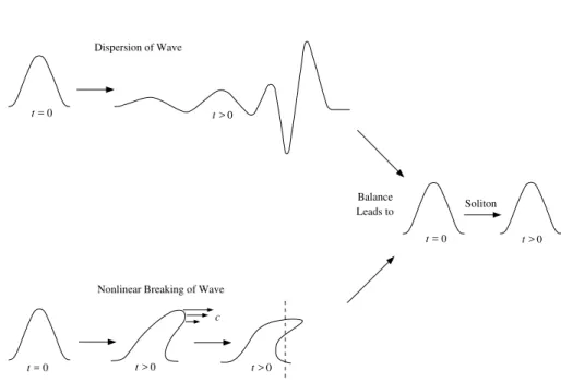
Thisisapuredispersivesolution. InFig. 3weseethat
a initial onguration at t = 0 will disperse as time
goes on. Eliminating the dispersive term we get the
purenonlinearequation
u
t =uu
x
(30)
Itanbeeasilyhekedbysubstitutionthat
u(x;t)=f(x ut) (31)
with f arbitrary,satises (30). From this solutionwe
onludethattheveloityof apointof thewave,with
onstantamplitudeu,isproportionaltoits amplitude
leadingtothe\breaking"ofthewave,asshowninFig.
3. Thewavealsodevelopsdisontinuities(indiatedby
thevertialdashedlineinFig. 3)in itsevolution. The
\mirale"ofthesolitonsolutionisduetoabalane
be-tweenthedispersionandthebreakingofthewave,both
phenonemaplaedtogetherleadtothewaveproleto
propagatewithouthangingitsshape.
t =
0
t >
0
t =
0
t >
0
t >
0
t =
0
t >
0
Nonlinear Breaking of Wave
Dispersion of Wave
Soliton
Balance
Leads to
c
Figure3.Thebalaneeetsofdispersionandbreakinginasoliton.
Equation (30) is alled the dispersionless KdV or
Riemann equation [19℄. The interesting fat is that
this equation is aintegrable Hamiltoniansystem. We
will return to study this equation in the next setion
but for themoment letus analysehowweget
disper-sionlessequations. Dispersionlessequationsanbe
ob-tained by onstrution oras a quasi-lassial limit of
integrable ones [20℄ . In the latter ase we make the
saling
t
!
t ,
x
!
x
andtakethelimit!0.
FortheKdVequation(2)(wewillhangetheonstant
fatorsonit, soinsteadof(5)wehaveL= 2
+uand
B= 3
+ 3
4
(u+u))
4u
t =u
xxx +6uu
x
) 4u
t =
3
% 0
u
xxx +6u
x u
+ u
t =
3
2 uu
x
KdV +
Riemann
This is like the WKB aproximation in quantum
me-hanisandwewilluseitasourguideline[20℄.
Dispersionless integrable systems were introdued
by Lebedev and Manin [21℄ and Zakharov [22℄, and
although interesting on their own started to appear
netion between2-dimensional eld theories and
inte-grableequationsofhydrodynamialtype[23-25℄(whih
are dispersionless systems). In2-dimensional
topolog-ialeld theories[26℄ we areinterested in alulating,
from thepartition funtion
Z
M =
Z
[d℄e S[℄
(32)
theorrelationfuntions
h
(x)
(y)i
M =h
i
M
(33)
whihdependonlyonthetopologyofthemanifoldM.
The2-pointand3-pointorrelationfuntionsaregiven
respetivelyby[27℄
h
i=
=nondegenerateonstant
h
i=
(t)=
3
F(t)
t
t
t
;;=1;2;:::;n (34)
where t = (t 1
;t 2
;:::;t n
) are the oupling onstants and F(t) is the free energy. The orrelations (34) dene a
ommutativeandassoiativealgebra(withanidentity)
e
Æe
=
e
(35)
withe
deningabasisforthealgebra. Theassoiativityofthealgebra,(e
Æe
)Æe
=e
Æ(e
Æe
),gives
3
F(t)
t
t
t
3
F(t)
t
t Æ
t
=
3
F(t)
t
t
t
3
F(t)
t
t Æ
t
(36)
d
These are the Witten-Dijkgraaf-Verlinde-Verlinde
(WDVV) equations [26,27℄and an beidentied with
equations of hydrodynami type. So, solutions of
hy-drodynamiequation anbeidentied with partiular
solutionsofthetopologialeld theory[25℄.
IV Two-Component
Hyper-boli Systems
In a series of papers [28-31℄Nutku and ollaborators
started to study dispersionless systems of equations
that arein-betweenthesimple Riemann equation[19℄
and themoregeneralequationsofhydrodynami type
[24℄
Riemann
TwoComponentHyperboli
Equationsof HydrodynamiType
u i
t =V
ij
(u)u j
x
i;j=1;:::;n
InFig. 4weanndahartwiththemainequations,
of thetwo-omponenthyperbolisystemtype,studied
onthesepapers.
A wealth of results onerning the integrabilityof
these systems were revealled. Innitely many
onser-vation lawsandmulti-Hamiltonian strutureswere
ob-tained. Inthissetionwewillbeinterestedinreprodue
someof these resultsfrom analgebraipoint of view.
InordertoahivethisgoalwemustunderstandtheLax
representationforthesesystems.
IV.1 Riemann Equation
TheRiemannequation
u
t =
3
2 uu
x
(37)
istheprototypeforthehyperbolisystems. Weaddress
thefollowingquestion: IsthereaLaxrepresentationfor
(37)? Yes, and we anobtainit performing the
semi-lassial limit [20℄ explained in Setion 3. So, if the
KdV equation goes to the Riemann equation (37) in
the semilassial limit, the Lax operator L = 2
+u
and B = 3
+ 3
4
(u+u) goesto thepolynomialsin
thevariablep
E =p 2
+u
M =p 3
+ 3
2
up (38)
andtheLaxrepresentation(4)goesto
E
alled dispersionless Lax representation (note the
re-semblanewhenwepassfromquantumtolassial
me-hanisdoing!pand[; ℄!f;g). Here
fA(x;p);B(x;p)g= A
p B
x B
p A
x
(40)
is thedispersionless Poisson braket[21,22℄. So, ifwe
substitute(38)in(39)weget(37).
Fromnowonwewill apply someof thetehniques
desribedin [17℄and[18℄ inaveryinformalway, sine
we wantto giveonly aavor of howthe \mahinery"
works.
Let us alulate the square root of E in (38). So,
wewritetheLaurentpolynomial
E 1=2
=p+a
0 +a
1 p
1
+a
2 p
2
+a
3 p
3
+ (41)
andfrom E=E 1=2
E 1=2
weobtaina
0 ;a
1 ;a
2 ;a
3 ;:::,or
equivalently,weperformaseriesexpansionforp!1
E 1=2
=
p 2
1+ u
2 1=2
p!1
= p+ 1
up 1
1
u 2
p 3
+ 1
u 3
p 5
5
u 4
p 7
Nowwealulate E 3=2 =E 1=2 E, E 5=2 =E 1=2 E 2 and soon E 3=2 =p 3 + 3 2 up+ 3 8 u 2 p 1 +::: E 5=2 =p 5 + 5 2 up 3 + 15 8 u 2 p+ 5 16 u 3 p 1 + . . . (43)
ThesetofgeneralLaurentpolynomialA= P +1 i= 1 a i p i
givesrisetoanassoiativealgebrag=fAg. This
alge-braanbewritten asadiretsumg=g
+
g ,where
g
+ =fA
+
gand g =fA gwith A
+ = P i0 a i p i and A = P i<0 a i p i
, respetively. Weanreognize M in
(38)as
M=(E 3=2
)
+
(44)
Infat,from(39)wearemotivated towrite
E t =f(E 1=2 ) +
;Eg ) u
t =u x E t =f(E 3=2 ) +
;Eg ) u
t = 3 2 uu x E t =f(E 5=2 ) +
;Eg ) u
t = 15 8 u 2 u x . . . (45)
and we havea hierarhy of equations. We all it
dis-persionlessKdV(orRiemann)hierarhyandwewrite
E t k =f(E 2k +1 2 ) +
;Eg; k=0;1;2;3;::: (46)
treatinguasafuntion ofk+1variables
u=u(x;t
0 ;t
1 ;t
2
;:::) (47)
Foreaht
k
wehavewhatisalledaowanditanbe
shownthattheyommute
2 E t ` t k = 2 E t k t ` (48)
onsequently, the whole set of equations (45) is
inte-grable sine, as wehavealreadypointed out,the
Rie-mannequationisanintegrableHamiltoniansystem(all
the equations in (45)share thesame set of onserved
harges).
TheRiemann equationanbeputintheform
u t = 3 2 uu x = 3 4 (u 2 ) x (49)
It followsthat thequantity H / R dxu 2 isonserved. R n
Theseonservedhargesanalso beobtainedfrom E.
LetbeAanygeneralLaurentpolynomial
A=+a
1 p
1
+ (50)
following[18℄weintroduetheAdler'straeas
TrA= Z
dxResA= Z
dxa
1
(51)
whihsatisestheusualrelationTrAB=TrBA. From
(42)and(43)weseethat
TrE 1=2 = 1 2 Z dxu TrE 3=2 = 3 8 Z dxu 2 TrE 5=2 = 5 16 Z dxu 3 . . .
andwehave
H n = 2 n TrE n=2
| {z }
p!1 (52) with _ H n
= 0. From a Hamiltonian point of view the
Riemannequationisaquadri-Hamiltoniansystem[30℄.
ThereareHamiltonianoperatorsD
1 ,D 2 ,D 3 whihare
ompatibleandanotherHamiltonianoperatorE whih
isompatibleonlywithD
1
. Weanwrite
u t =D 1 ÆH 5 Æu =D 2 ÆH 3 Æu = 3 4 D 3 ÆH 1 Æu = 35 8 E ÆH 9 Æu (53) where H 1 = R
dxu; D
1 =2 H 3 = 1 4 Z dxu 2 ; D 2
=u+u
H 5 = 1 8 Z dxu 3 ; D 3 =u 2 +u 2 H 9 = 7 128 Z dxu 5
; E = 1 u x 1 u x (54)
Hamiltonianstrutures analso beobtained from the
Lax operator L (E in the dispersionless ase). They
arethesympletistruturesofKostant-Kirillov[32℄on
theorbitsoftheoadjointrepresentationofLiegroups
[18,33℄. Fordispersionlessequationstheorresponding
Liealgebrais givenby theassoiativealgebraof
Lau-rent polynomialsendowed with the braket (40). For
theKdVequationtheLiealgebraisgivenbythe
struturesD
1 ,D
2 ,D
3
anbederived(see[4℄fordetails)
whilewewere notabletoobtainE fromthissheme.
IV.2 Polytropi Gas Equation
WewilltrytoapplytheresultsofthelastSetionto
someothers dispersionlessequations, suhasthe ones
in the hart of Fig. 4. The polytropi gas dynamis
equation
u
t +uu
x +v
2
v
x =0
v
t +(uv)
x =0
2 (55)
was studied from aHamiltonian pointof view in [30℄.
In (55) u is the veloity of the uid, v is its density,
f =v 2
andis relatedto thepressure(f(v)= p
0
(v)
v )
andistheratioofspei heats(weallanidealgas
polytropiifthespeiheatsareonstantoveralarge
rangeoftemperature).
TherststepwillbetoderiveaLaxrepresentation
for(55). Wegetahintifweonsider=2in(55). In
this asewehavetheshallowwater equation[19℄ also
known astheirrotational Benney equation [34℄. Even
though we do not know the dispersive system whih
originates (55) for any we do know it for the ase
=2. This is thedispersive shallowwater[35℄
equa-tion,alsoalledthetwobosonequationineld theory
J
0
t
=(2J
1 +J
2
0 +J
0
0 )
0
J
1
t
=(2J
0 J
1 +J
0
1 )
0
(56)
This equationhas thefollowingnonstandardLax
rep-resentation[36,37℄
L= J
0 +
1
J
1
L
t
=[L;(L 2
)
1
℄ (57)
where(L 2
)
1
standsforthepurelynonnegative
(with-outp 0
terms)partof thepolynomialin pandJ
0 /u,
J
1
/v are the twobosonselds. Now, if we perform
thesemilassiallimitand dotheappropriate
identi-ations(56)yields(55)for=2andfrom(57)weget
thefollowingdispersionlessLaxrepresentation
L =p+u+vp 1
L
t =
1
2 f(L
2
)
1
;Lg (58)
For any wean use(58) asan ansatzto obtain the
dispersionless Laxrepresentationfor (55)and itreads
[5℄
L = p 1
+u+ v
1
( 1) 2
p ( 1)
L
t =
( 1)
L
1
1 ;L
(59)
In[30℄twosetsofonservedhargeswerederivedfor
(55) when 6=2. So,if (59)is really the orret Lax
pairitmustsomehowprovidebothsets aordinglyto
the algebraisheme desribed in the last setion. In
fat, sineL hassingularities in p=0and p=1we
an expand L 1
1
in powers of p in the twofollowing
ways
L 1
1
=p (
1+ 1
1
up ( 1)
+ v
1
( 1) 2
p 2( 1)
+
(2 )
2( 1) 2
h
i
2
+
+
(2 )(3 2)
6( 1) 3
h
i
3
+ )
p!1 (60a)
L 1
1
= vp
1
( 1) 2
1 (
1+ 1
1
h
( 1) 2
v ( 1)
up ( 1)
+p 2( 1)
i
+
+
(2 )
2( 1) 2
h
i
2
+
(2 )(3 2)
6( 1) 3
h
i
3
+ )
p!0 (60b)
So,therstsetofhargesfollowsfrom
H
n =TrL
n+ 2
1
| {z }
p!1 =
R
dxH
where therstdensitiesare
H
0 =
( 2)
( 1) u
H
1 =
(2 3)( 2)
( 1) 2
1
2! u
2
+
1
( 1)( 2) v
1
H
2 =
(3 4)(2 3)( 2)
( 1) 3
1
3! u
3
+
1
( 1)( 2) uv
1
.
.
.
H
n
=(n+1)!C
(n+1)( 1) 1
( 1)
n+1
H
n+1
(62)
and
H
n =
[ n
2 ℄
X
m=0 m
Y
k =0 1
k( 1) 1
!
u n 2m
m!(n 2m)! v
m( 1)
( 1) m
(63)
whiharetherstsetofhargesobtainedin [30℄. Theseond setfollowsfrom
e
H
n =TrL
n+ 1
1
| {z }
p!0 =
R
dx e
H
n
n=0;1;2;3;::: (64)
andtherstdensitiesare
e
H
0
=( 1) 2
1
v
e
H
1
=( 1) 2
1
( 1) uv
e
H
2
=( 1) 2
1
(2 1)
( 1) 2
1
2! u
2
v+ v
( 1)
.
.
.
e
H
n =
n!
( 1) 2
1 C
n( 1)+1
( 1)
n
e
H
n
(65)
where
e
H
n =
[ n
2 ℄
X
m=0 m
Y
k =0 1
k( 1)+1 !
u n 2m
m!(n 2m)! v
m( 1)+1
( 1) m
(66)
d
istheseondset ofhargesobtainedin[30℄
In(59)L 1
1
wasexpandedin p=1,aexpansion
around p=0provides aseond onsistent
dispersion-lessLaxequation
L
t =
L 2
1
0 ;L
(67)
whihyields(withtheproperresaling)theequations
u
t =v
3
v
x
v
t =u
x
(68)
FromthehartinFig. 4wereognizethisequationsas
IV.3 Born-Infeld Equation
WiththeLaxrepresentationforthepolytropigas,
obtainedinthelastsetion,weangetaLax
represen-tation forthe Born-Infeld equation given in the hart
ofFig. 4
u
t =
1
u 2
+ 1
v 2
u
x 2u
v 3
v
x
v
t =
1
v 2
+ 1
u 2
v
x 2v
u 3
u
In(69)theBorn-Infeldequationisexpressedinthe
so alled null oordinates version [31℄. If we perform
thetransformation u= x v = x p 1+ x t (70)
weobtaintheBorn-Infeldequationwrittenasa
seond-orderequationin nulloordinates
2 x tt + 2 t xx
(4+2
x
t )
xt
=0 (71)
ALaxrepresentationfor(69)anbeobtainedasfollows
[6℄. Intherstplaeifwedothehange ofvariables
e u= (u
2 +v 2 ) e v= 1 2 uv (72)
alledVeroskytransformation[31℄,wewillendupwith
theequation
e u
t +ueeu
x + e v x e v 3 =0 e v t +(euev)
x
=0 (73)
knownastheChaplygingas. Inviewofthisitwouldbe
desirabletorstobtainaLaxdesriptionofthe
Chap-lygingaslikeequations
e u
t +eueu
x + e v x e v +2
=0; 1
e v
t +(eu ev)
x
=0 (74)
Thisisindeedpossibleifweset! ,1in(59),
so(74)anbeobtainedfrom
L=p (+1)
+ue+ e v
(+1)
(+1) 2 p +1 L t =
(+1)
n L +1 1 ;L o (75) whereL 1 +1
isexpandedaroundp=0and L
+1
1 is
thepolynomialinpthatproduesonsistentequations,
instead of the purely nonnegative polynomial used in
(59). For=1theLaxoperator
L=p 2 1 u 2 + 1 v 2 + 1 u 2 v 2 p 2 L t =2 L 1 2 1 ;L (76)
reprodues(69). Again,onservedhargesfollowsfrom
e
H
n =TrL
n 1
2
| {z } = Z dx e H n
n=0;1;2;3;::: (77)
andtherstBorn-Infeldhargesare
e H 0 = uv e H 1 = 1 2 u v + v u e H 2 = 3 4 u 2v 3 + 3 uv + v 2u 3 . . . (78)
and these areexatlythe hargesderivedin [31℄.
An-otherset isobtainedfrom
H
n =TrL
n+ 3
2
| {z }
p!0 =
Z
dxH
n
n=0;1;2;3;::: (79)
andtherstonesare
H 0 = 3 2 1 u 2 + 1 v 2 H 1 = 15 8 1 u 4 + 11 6 1 u 2 v 2 + 1 v 4 H 2 = 35 16 1 u 6 1 u 4 v 2 1 u 2 v 4 + 1 v 6 . . . (80)
Thisisanewsetofonservedharges,forthe
Born-Infeldequation(69),notfoundpreviouslyin [31℄.
V Conlusions
Webelieve,from theresultsof theSetion 4,that the
studyofdispersionlesssystemsviaaLaxrepresentation
is worthwhile. So, the searh for a dispersionless Lax
representationfortheequationsintheupperpartofthe
hartinFig. 4isbeingpursued. Also,thederivationof
the multi-Hamiltonian strutures of these systems, as
desribedin[28-31℄,isunderinvestigationfollowingthe
oadjointorbitmethod [32,33℄. Anotherquestionthat
omesto mindisthedispersivegeneralizationofthese
equations. Attemptsin this diretion anbefound in
[38℄.
Sometopologialequationsarealsorelatedwiththe
systems disussed here. For instane, the hyperboli
Monge-Ampereequation
U tt U xx (U tx ) 2
= 1 (81)
mayberelatedwiththeBorn-Infeldequationasfollows.
a=U
x
b=U
t
(82)
the Monge-Ampere equation an be written as a
rstordersystem
a
t =b
x
b
t =
b 2
x 1
a
x
(83)
and thisequation anberelated totheChaplygin gas
equation(73)throughthefollowinghangeofvariables
e u=
b
x
a
x
e v =a
x
(84)
Thus, we an give a Lax desription for the
hyper-boliMonge-Ampere equation throughthe Lax
repre-sentation derivedin Setion 4.3. Finally, the
Witten-Dijkgraaf-Verlinde-Verlinde (WDVV) equations (36),
forn=3,with
F(t 1
;t 2
;t 3
)= 1
2 (t
1
) 2
t 3
+ 1
2 t
1
(t 2
) 2
+f(t 2
;t 3
) (85)
where t 2
xandt 3
t,yieldsthethird order
Monge-Ampere equation
f
ttt =f
2
xxt f
xxx f
xtt
(86)
Thisequationisabi-Hamiltoniansystemandhasa
ma-trixLaxrepresentation. Itisthenpossibleto generate
awholesetofnonloalhargesmuhlikethenonlinear
sigmamodel(details aregiven in[7℄). It islikelythat
adispersionlesssortofLaxrepresentationfor(86)may
exist.
Aknowledgments
Iwouldliketo thankAshokDasandCelsoM.
Do-riaforusefuldisussions. This workwassupported by
CNPq, Brazil.
Referenes
[1℄ L.D.FaddeevandL.A.Takhtajan,Hamiltonian
Meth-odsintheTheoryof Solitons,Springer-Verlag,1987.
[2℄ A.Das,Integrable Models,WorldSienti,1989.
[3℄ P.G.DrazinandR.S.Johnson,Solitons: an
Introdu-tion,CambridgeUniversityPress, 1989.
[4℄ J.C.Brunelli,HamiltonianStruturesforthe
General-ized Dispersionless KdV Hierarhy, Rev.Math. Phys.
[5℄ J.C.BrunelliandA.Das,ALaxDesriptionfor
Poly-tropi Gas Dynamis, Phys. Lett. A235, 597 (1997)
(solv-int/9706005).
[6℄ J.C. Brunelli and A. Das, A Lax Representation for
theBorn-InfeldEquation,Phys.Lett.B426,57(1998)
(hep-th/9712081).
[7℄ J.C.BrunelliandA.Das,Non-loalChargesandtheir
AlgebrainTopologialFieldTheory,Phys.Lett.B438,
99(1998)(hep-th/9802070).
[8℄ J.Sott-Russell,ReportonWaves,14thMeetingofthe
British Assoiation for the Advanement of Siene,
JohnMurray,London,1844,p.311.
[9℄ D.J.KortewegandG.deVries,OntheChangeofForm
ofLongWavesAdvaninginaRetangularCanal,and
onaNewTypeofLongStationaryWaves,Philos.Mag.
39,422(1895).
[10℄ E. Fermi,J. Pasta and S.M. Ulam,Studies in
Non-linearProblems,Teh.Rep.LA-1940,LosAlamosSi.
Lab.(alsoinColletedPapersofEnrioFermi,Vol.II,
1965,p.978,ChiagoUniversityPress).
[11℄ N.J.ZabuskyandM.D.Kruskal,Interationof
\Soli-tons"inaCollisionlessPlasmaandtheReurrene of
InitialStates, Phys.Rev.Lett.15,240(1965).
[12℄ C.S. Gardner, J. M. Greene, M. D. Kruskaland R.
M. Miura, Method for Solving the Korteweg-de Vries
Equation,Phys.Rev.Lett.19,1095(1967).
[13℄ P.D. Lax,Integrals ofNonlinearEquations of
Evolu-tionandSolitaryWaves,Comm.PureAppl.Math.21,
467(1968).
[14℄ C.S.Gardner,Korteweg-de Vries Equation and
Gen-eralizations.IV.TheKorteweg-deVriesEquationasa
HamiltonianSystem,J.Math.Phys.11,1548(1970).
[15℄ V.E.ZakharovandL.D.Faddeev,Korteweg-de Vries
Equation: A Completely Integrable Hamiltonian
Sys-tems,Fun.Anal.Appl.5,280(1971).
[16℄ F.Magri, A Simple Model of the Integrable
Hamilto-nianEquation, J.Math.Phys.19,1156 (1978).
[17℄ I. M. Gel'fand and L. A. Dikey, Asymptoti
Be-haviourof theResolvent of Sturm-LiouvilleEquations
and the Algebra of the Korteweg-de Vries Equation,
Russ.Math.Surveys30,77(1975).
[18℄ M.Adler,On aTraeFuntionalforFormal
Pseudod-ierential Operators and the Sympleti Struture for
theKorteweg-de Vries Type Equations, Invent.Math.
50,403(1979).
[19℄ G. B. Whitham, Linear and Nonlinear Waves, John
Wiley&Sons,1974.
[20℄ V.E.Zakharov,Benney Equations andQuasilassial
Approximationin the Method of the Inverse Problem,
Funt.Anal.Appl.14,89(1980).
[21℄ D.LebedevandYu.I.Manin, ConservationLawsand
LaxRepresentationonBenney'sLongWaveEquations,
Phys.Lett. 74A,154(1979).
[23℄ I. Krihever, The Dispersionless Lax Equations and
TopologialMinimalModels,Comm.Math.Phys.143,
415(1992);The-Funtion oftheUniversalWhitham
Hierarhy, Matrix Models and Topologial Field
The-ories, Commun. Pure Appl. Math. 47, 437 (1994);
WhithamTheory forIntegrableSystemsandTopolo
gi-alQuantumFieldTheories,inNewSymmetry
Prini-plesinQuantumField Theory,p.309,ed.J.Frohlih
etal.,PlenumPress,NewYork,1992.
[24℄ B.A.Dubrovinand S.P.Novikov, Hydrodynamis of
Weakly Deformed SolitonLatties. Dierential
Geom-etry andHamiltonian Theory, Russ. Math. Surv. 44,
35(1989).
[25℄ B. Dubrovin, Integrable Systems in Topologial Field
Theory,Nul.Phys.B379,627(1992);Geometryof2D
TopologialFieldTheories,preprintSISSA-89/94/FM,
SISSA,Trieste,1994, hep-th/9407018.
[26℄ E. Witten, On the Struture of the Topologial Phase
of Two-Dimensional Gravity, Nul. Phys.B340, 281
(1990).
[27℄ R.Dijkgraaf,H.VerlindeandE.Verlinde,Topologial
Stringsind<1,Nul.Phys.B352,59(1991).
[28℄ Y. Nutku, On a New Class of Completely Integrable
NonlinearWaveEquations.I.InnitelyMany
Conser-vationLaws,J.Math.Phys.26,1237(1985).
[29℄ Y. Nutku, On a New Class of Completely Integrable
Nonlinear Wave Equations. II. Multi-Hamiltonian
Struture,J.Math.Phys.28,2579(1987).
[30℄ P.J.OlverandY.Nutku, HamiltonianStrutures for
Systems of Hyperboli Conservation Laws, J. Math.
Phys.29,1610(1988).
[31℄ M. Arik, F. Neyzi, Y. Nutku, P. Olver and J. M.
Verosky, Multi-Hamiltonian Struture of the
Born-InfeldEquation, J.Math.Phys.30,1338 (1989).
[32℄ A.A. Kirillov,Elementsof theTheory of
Representa-tions,SpringerVerlag,1976;B.Kostant,Quantization
and Unitary Representation, part I: Prequantization,
Let. Notes in Math. 170, 87 (1970); J. M. Souriau,
Struturedes SystemsDynamiques,Dunod,1970.
[33℄ B.Kostant,Quantization and Representation Theory,
London Math. So. Let. Notes 34, 287 (1979); A.
G. Reyman, M. A. Semenov-Tian-Shansky and I. B.
Frenkel, Graded Lie Algebras and Completely
Inte-grableSystems,Sov.Math.Dokl.20,811(1979);A.G.
ReymanandM.A.Semenov-Tian-Shansky,Redution
of Hamiltonian Systems, AÆneLie Algebrasand Lax
Equations. I andII,Invent. Math. 54,81(1979) and
63,423(1981);W.W.Symes,Systems ofToda Type,
Inverse SpetralProblems andRepresentationTheory,
Invent.Math.59,13(1980);D.R.LebedevandYu.I.
Manin,Gelfand-DikiiHamiltonianOperatorand
Coad-joint Representation of Volterra Group, Funt. Anal.
Appl.13,268(1980).
[34℄ D. J. Benney, Some Properties of Long Nonlinear
Waves,Stud.Appl.Math.52,45(1973).
[35℄ L.J.F.Broer,ApproximativeEquationsforLong
Wa-terWaves,Appl.Si.Res.31,377(1975);D.J.Kaup,
AHigher-OrderWater-WaveEquationandtheMethod
forSolvingIt,Progr.Theor.Phys.54,396(1975).
[36℄ B.A.Kupershmidt,Mathematis ofDispersiveWater
Waves,Commun.Math.Phys.99,51(1985).
[37℄ J.C.Brunelli,A.DasandW.-J.Huang,Gelfand-Dikii
Brakets for Nonstandard Lax Equations, Mod.Phys.
Lett.9A,2147(1994).
[38℄ B.Enriquez,A.YuOrlov andV.N.Rubtsov,
Disper-sionfulAnaloguesof Benney'sEquations andN-Wave