Current Distribution in Fused Electrical Networks
J.S. Espinoza Ortiz
1and Gemunu H. Gunaratne
1,21
Department of Physics, University of Houston, Houston, TX77204
2
The Institute of Fundamental Studies, Kandy 20000, Sri Lanka
Received on 27 December, 2002
Electrical networks provide a natural model to study transport processes such us dielectric breakdown and metal insulator transition in disordered inhomogeneous conductors. We present a calculation for current distribution on an infinite hyper-cubic network due to an external applied current. This is used to compute, analytically, the redistribution of current due to variations in the conductance of a finite number of elements of the network.
1
Introduction
Electrical network models can be used to study transport phenomena in disordered systems. Examples of such sys-tems include compacted mixtures of conducting and non-conducting materials or homogeneous multi-phase system with varying conductivity. Applications to disordered net-works cover dielectric breakdown [1, 2, 3], metal-insulator transitions [4], and brittle fracture in disordered solids [5, 6, 7, 8]. In particular,such models have provided insights on critical phenomena [9], scale-invariant disorder [10, 9, 3], and size-dependence of the system [11]. In this paper we introduce an exact analytical technique to compute current distributions on model networks.
In the “Effective Medium Theory”, the distribution of current in a random network of conductances to which an external current has been applied along a fixed direction must be regarded as due to both an “external field” which in-creases the mean current, and a “fluctuating local field” due to deviations from a uniform medium. The “mean current” is chosen so that the average of these fluctuation vanish.
We consider fused-conducting networks, where the breakdown currents of an element is assumed to be propor-tional to its conductance; i.e., breakdown of any conductor occurs when the potential difference across it reaches a fixed pre-set value. In the simplest case, conductances along each axis of a hyper-cube are set equal. In Section II, we calculate how an external current introduced at a node and removed from an adjacent node is distributed on the network [12, 13]. The Green’s Function derived for this case can be used to calculate the current distribution due to an external field on a network from which a finite number of conductances are removed. Several examples are shown in Section III, for two and three dimensional networks. Subsequently, in section IV, this method is generalized to consider networks where conductances are reduced (as opposed to vanishing) beyond a critical current. Section V presents discussions and con-clusions.
2
Green’s Functions for Hyper-cubic
Network
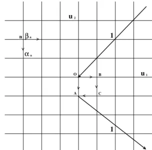
Lets us consider an infinited-dimensional hyper-cubic net-work where all conductances along themth direction (uˆ
m)
are assumed to be equal to σm(m = 1,2, ..., d). In this section we calculate the distribution of current on this net-work due to a unit external current introduced at the ori-gin and removed from an adjacent node, say a. This result
was obtained by using a Green’s function method by Kirk-patric [12, 11] and is reproduced here for completeness.
u1
u2
O
A B
C
1
1 β
α
n
n
n
Figure 1. Scheme to compute the current distribution due to a unit external current introduced at the origin and removed from an ad-jacent node.
Denote the potential at the node n= (n1, n2, ..., nd),
by V(n) and the current on the conductor joining nodesn
andn+uˆm by Jm(n); then,
The potentials V(n) can be obtained using the Kirchhoff’s rule at each node; i.e., d
m=1 σm {[V(n)−V(n+ˆum)]
+ [V(n)−V(n−uˆm)]}= (δn,0−δn,a),
(2)
where the term in the right side is the externally applied current. Eqn. (2) is easily solved by using the Fourier transform
ˆ
V(k) =
ne−
in k
V(n),which satisfies d
m=1 2σm[1−cos(ˆum·k)] ˆV(k) =1−e−ia k.
Thus
ˆ
V(k) = (1−e
−ia k)
d
m=12σm[1−cos(km)], (3)
wherekm=uˆm·k. Hence
V(n) = 1/2
(2π)d
π −π dke
in k ˆ
V(k), (4)
and
Jm(n) = σm 2 (2π)d
π
−π eink
1−e−ika−eikm+ei(km−ka) d
m′=1σm′[1−cos(km′)]
dk. (5)
Next, let us specialize to networks in two dimensions with equal conductances (σm = 1), and definea = ˆu2, α(n) ≡
Jy(n) and β(n) ≡ Jx(n), see Fig. 1. In order to obtain expressions forα′sandβ′sis also necessary to consider implicit symmetries on the networks; i.e.,
α(nx,ny)= α(nx,−ny)= α(−nx,ny)= α(−nx,−ny),
β(nx,ny)= −β(nx,−ny)= −β(−nx,ny)= β(−nx,−ny).
(6)
These are easily obtained by taking into account the flux of current in theOABCcell and by reflecting it with respect toOA, see Fig. 1.
Combining Eqns. (5) and (6) gives α(n)=π12
π 0
[1−cos(ky)] cos(nxkx) cos(nyky)
2−cos(kx)−cos(ky) d k,
β(n)=π22
π 0
sin(kx/2) sin(ky/2) sin [(nx+1/2)kx]
2−cos(kx)−cos(ky)
×sin [(ny+ 1/2)ky]dk.
(7)
This analysis can be easily extended to compute theα’s andβ’s in three dimensions. These are calculated using configu-ration analogous to Fig. 1 with the unit external current is introduced along theuˆ3direction. Then
α(n)= π13
π 0
[1−cos(kz)] cos(nxkx) cos(nyky) cos(nzkz)
3−cos(kx)−cos(ky)−cos(kz) d k,
βx (n)=
2 π3
π 0
sin(kx/2) sin(kz/2) sin[(nx+1/2)k] cos(nyky)
3−cos(kx)−cos(ky)−cos(kz)
×sin[(nz+ 1/2)k]dk,
βy(n)=
2 π3
π 0
sin(ky/2) sin(kz/2) cos(nxkx) sin[(ny+1/2)k]
3−cos(kx)−cos(ky)−cos(kz)
×sin[(nz+ 1/2)k]dk.
(8)
⌈
Notice, now there are two possible directions forβ′s (i.e. x andy, respectively).
Values of α’s and β’s given by Eqn. (7-8) for several
nare given in the Appendix, and will be used for
computa-tion to follow. In particular α0= 1/2and 1/3 in two and
three dimensions respectively, as can be easily confirmed us-ing arguments based on symmetry and superposition [12] .
expanding the denominator as a series in powers of coskj. Expansion to fourth order gives results that are accurate to within2%.
3
Removal of Conductors in
Net-works
In this section we introduce a method to calculate the current distribution on the network when a finite number of
conduc-tances are removed.
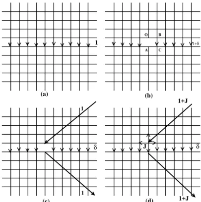
Consider a two dimensional isotropic(σx = σy = 1) network with an externally applied unit electric field in the y−direction. The currents on this configuration are Jx(n) = 0, Jy(n) = 1,see Fig. 2(a).
(a) (b)
(c) (d)
δ
1
1+δ
1
1
J δ
1+J
1+J
O
A B
C
Figure 2. Scheme to compute the current distribution when a single conductance is removed. In sequence:(a) an isotropic network with a current flow along they−direction. In (b) a conductance is removed , andδis the excess of current in a remaining element. Next in (c) , a
unit external current is introduced in order to computeδ. Finally (d) shows the configuration from whichδcan be evaluated.
First, we enumerate changes in the current distribution due to the removal of the conductor joining the origin to
(0,−1), the linkOAin Fig. 2(b). The excess currentδon any remaining element can be considered to be the redistri-bution of the current that originally passed through the link OA , i.e.(0,0)−(0,−1), see Fig. 2(c). δ can be evalu-ated using specific values of α’s and β’s by the following procedure. Consider the complete network, with and exter-nal current(1 +J)introduced at(0,0)and removed from
(0,−1), as shown in Fig. 2(d). (1 +J)is chosen so that a currentJpasses through(0,0)−(0,−1), and the remainder
(= 1)passes through the rest of the network; i.e., this sec-ond part is the solution to the problem illustrated in Fig. 2(c). But from the discussion in Section II, the current passing through(0,0)−(0,−1)isα(0,0)×(1 +J). Hence,
J =α(0,0)×(1 +J). (9)
Sinceα(0,0)= 1/2, we find thatJ = 1and that the changes
of current in the network are given by,
△Jy(n) = (1 +J)α(nx,ny) = 2α(nx,ny),
△Jx(n) = (1 +J)β(nx,ny) = 2β(nx,ny).
(10)
In particular , the current on conductances adjacent to that removed in Fig. 2(b) is
Jmax = 1 + 2α(1,0) = 4/π ,
as was given by Duxbury et. al. [11]
Finally, we provide results from the analogous calcula-tion for cubic networks of fused conductances. For a single fracture like in Fig. 2,J = 1/2 and the value of maxima current for adjacent links are,
Jmax = 1 +α(1,0,0)(1 +J) = 1 +α(0,1,0)(1 +J)
= 1 +α(0,0,1)(1 +J) = 1.092625. (11)
4
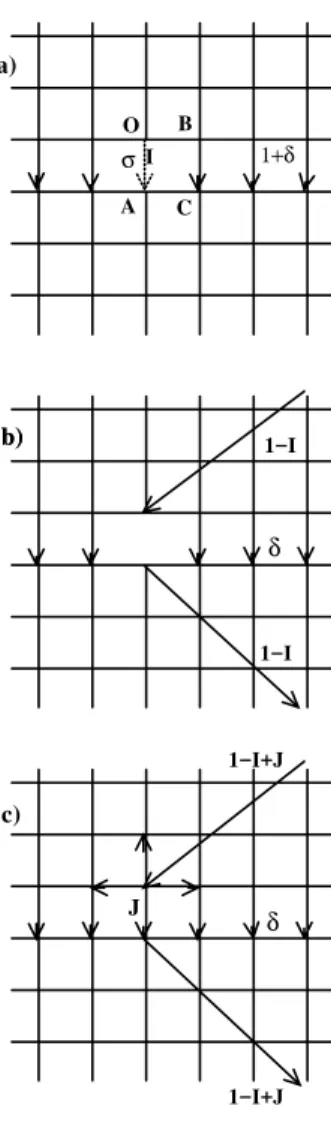
Reduction of Conductances
The next problem we address is how the current distribu-tion of the network changes if the conductance of one bond changes to σ <1,while the remaining conductors are left unchanged. The current passing thorough this link will de-crease causing the remainder to be re-distributed onto the rest of the network. We show how the values of these cur-rents can be calculated.
In Fig. 3(a) we consider the bondOAhas its conduc-tance reduced toσ, and there is a currentIpassing through it. The remainder(1−I)is redistributed into the network causing an excess of currentδon remaining elements. This is evaluated using a procedure schematically depicted in Fig. 3(c). Consider the complete network, and an external current(1−I+J)is applied atOand removed fromA. It is chosen so that a currentJ passes through the linkOAand the remainder(1−I)passes through the rest of the network. Because of this construction, the changes in the current on the cellOABC (in terms ofα′s and β′s) are (as was dis-cussed in Section II) ,
O B A C I 1−I 1−I 1−I+J 1−I+J δ δ 1+δ a) b) b) c) σ J
Figure 3. Procedure to compute the current distribution when a central conductance is reduced toσ(< 1). In (a) the conductance on the linkOAis set up to beσ and its current isI. Then the extra current around its neighborhood isδ. An external current(1−I)is
introduced in order to computeδ, in Figure (b). Finally (c) shows the configuration from whichδis evaluated.
J = α(0,0)(1−I+J), △Jx = β(0,0)(1−I+J), △Jy = α(1,0)(1−I+J), △J−x = −β(0,−1)(1−I+J).
(12)
Notice that in order to compute the variations of currents we introduced an auxiliary variable, and the solution require an additional condition. This is obtained by applying Kirck-off’s rule into the cellOABC. Thus,
VOA = VOB+VBC+VCA
I/σ = △Jx+ [1 +△Jy] +△J−x. (13)
Solving (12) and (13), we find
J= (1−σ)/(1 +σ), (14) and the changes in currents are:
I = 2σ/(1 +σ),
△Jx = 2β(0,0)(1−σ)/(1 +σ), △Jy = 2α(1,0)(1−σ)/(1 +σ), △J−x = −2β(0,0)(1−σ)/(1 +σ).
(15)
Notice that when σ = 0, we retain the results derived in Section III. O A B C D J J J 1 2 3
J −I
1+J −I 1+J −I
1 1 2 2 3 3 0.072 0.154 0.002 a) b) 0.17 0.173 0.017 1.137 0.877 1.031 1.116 I I I 1 2 3
Figure 4. A network with the three conductances (in dashed lines) set up equal to0.5, and current distributions on the boundary of this region. The scheme to compute the redistribution of current is shown in (b).
J1 = α(0,0)(J1−I1) +β(0,0)(1 +J2−I2) +β(1,0)(1 +J3−I3) ; J2 = −β(−1,0)(J1−I1) +α(0,0)(1 +J2−I2) +α(1,0)(1 +J3−I3) ; J3 = −β(−1,−1)(J1−I1) +α(−1,0)(1 +J2−I2) +α(0,0)(1 +J3−I3)
and,
I1/σ1 = [−β(0,0)+α(1,0)−β(0,−1)](J1−I1) + [−α(0,1)+β(0,1)
+ α(1,1)](1 +J2−I2) + [−α(1,1)+β(1,1)+α(2,1)](1 +J3−I3) ;
I2/σ2 = [−α(0,1)+α(−1,1)](J1−I1) + [−β(−1,0)+β(−1,−1)](1 +J2−I2) +I3
+ [−β(0,0)+β(0,−1)](1 +J3−I3) ;
I3/σ3 = [−α(0,2)−β(−1,2)+α(−1,2)](J1−I1) + [−β(−2,0)+α(−2,0)+β(−2,−1)](1 +J2−I2)
+ 1 + [−β(−1,0)+α(−1,0)+β(−1,−1)](1 +J3−I3).
⌈
The first set of equations are obtained imposing balance of current, and the last ones from applying Kirchoff’s laws. For particular case which considersσ1 =σ2 = σ3 = 0.5, some of the currents on the network are given again in Fig. 4(a) and their values were confirmed through numer-ical integrations on 100× 100 networks. Values for cur-rents on dashed bounds are:J1= 0.225;J2= 0.495;J3=
0.476,andI1 = 0.113;I2 = 0.748;I3 = 0.738, respec-tively.
Next let us provide another application considering two
clusters interacting, in Fig. 5. Setting up the following val-ues to conductivities: σ1 = 0.09, σ2 = 0.15, σ3 = 0.6, andσ4 = 0.9, we have solved numerically 8 linear equa-tions to obtain several values of currents which are shown in the same Figure. The respectiveJ’s values were: J1 =
0.0287, J2= 0.0133, J3= 0.2483, andJ4= 0.0767. Finally we consider the three dimensional fractured net-work depicted in Fig. 6. Using analogous arguments above, the currents are computed from:
⌋
J1 =α(0,0,0)(J1−I1) +β(y−1,0,0)(J2−I2) +β(0,1,y −2)(1 +J3−I3) ; J2 =β(0,1,0)x (J1−I1) +α(0,0,0)(J2−I2) +β(0,1,x −1)(1 +J3−I3) ; J3 =−βy(0,1,1)(J1−I1)−βx(0,−1,0)(J2−I2) +α(0,0,0)(1 +J3−I3),
and
I1/σ1 = [β(0,0,0)x +α(1,0,0)−β(0,0,x −1)](J1−I1) + [α(−1,0,0)+βy(−1,0,−1)−α(−1,1,0)](J2−I2)
+ [β(0,1,x −2)+β(1,1,y −2)−β(0,2,x −2)](1 +J3−I3),
I2/σ2 = [α(0,1,0)+β(0,1,x −1)−α(1,1,0)](J1−I1) + [βy(0,0,0)+α(0,1,0)
+ β(0,0,y −1)](J2−I2)−[βy(0,1,−1)+βx(0,2,−1)−β y
(1,1,−1)](1 +J3−I3), I3/σ3 = [β(0,2,1)x −β
y
(1,1,1)−β x
(0,1,1)](J1−I1) + [α(1,−1,0)−β(0,x −1,−1)−α(0,−1,0)](J2−I2)
+ [β(0,0,0)x +α(1,0,0)−β(0,0,x −1)](1 +J3−I3) + 1.
⌈
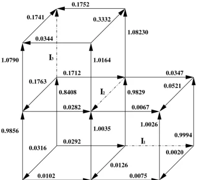
Setting up conductivities to beσ1= 0.5, σ2= 0.25 and σ3= 0.1we have obtainedI1 = 0.0091, I2 = 0.0083 and
0.0 2.0 4.0 6.0 0.0
2.0 4.0 6.0
0.0030 0.0867
0.0034 0.0868 0.0933 0.0233
0.0270 0.0027 0.0021
0.7545 1.0840
0.9698
0.9346 1.0056 1.0029 0.9775 0.9860
σ1 σ2
σ3 σ4
Figure 5. A network with four (reduced) conductances set up toσ1 = 0.09,σ2 = 0.15,σ3 = 0.6andσ4 = 0.9(in dashed lines). Some
currents on their neighborhood are also shown.
I
I
I
1 23
0.1741 0.3332
1.08230
1.0164 1.0790
0.1763
0.1712
0.0282
0.9856
0.8408
0.0316
0.0292
0.0067
0.0347
0.9829
0.0020
0.0075 0.0126 1.0035
0.9994 0.0521
1.0026 0.0344
0.1752
0.0102
Figure 6. A three-dimensional fractured network with three conductances settled up toσ1 = 0.5, σ2 = 0.25 andσ3 = 0.1(in dashed
5
Discussions and Conclusions
We have presented a method to compute current distribu-tions on infinite two and three dimensional networks, a fi-nite number of whose conductances differ from unity. The method can be used to calculate (for example) how break-down strength of a networks reduces due to a “fracture” of κcongruent locations whose conductances have “burned”. The expression obtained from this calculation can be
gen-eralized to elastic networks, one of whose applications is the determination of a relationship between the strength and density of the trabecular bone, with possible applications in using bone strength as a non-invasive diagnostic tool to iden-tify patients with osteoporosis [15, 16].
We would like to thank discussions with C. Rajapakse. This work is partially funded by the Office of Naval Research, the National Science Foundation and the ICSC -World Laboratory.
6
Appendix
Table 1: Values of severalα(nx, ny)’s. In particular α(0,0) = 1/2, and α(1,0) = 1/2(4/π−1). ny
nx 0 1 2 3 4 5
0 0.50000 0.13662 0.04648 0.02019 0.01080 0.00670 1 0.13662 0.00001 0.01455 0.01174 0.00816 0.00571 2 0.04648 0.01455 0.00000 0.00404 0.00441 0.00383 3 0.02019 0.01174 0.00404 0.00000 0.00162 0.00208 4 0.01080 0.00816 0.00441 0.00162 0.00000 0.00080 5 0.00670 0.00571 0.00383 0.00208 0.00080 0.00000 6 0.00457 0.00413 0.00314 0.00205 0.00113 0.00045
Table 2: Values of β for the first pairs of (nx, ny). ny
ny 0 1 2 3 4 5
0 0.18169 0.04507 0.01315 0.00469 0.00205 0.00106 1 0.04507 0.03052 0.01596 0.00826 0.00451 0.00264 2 0.01315 0.01596 0.01192 0.00789 0.00510 0.00334 3 0.00469 0.00826 0.00789 0.00626 0.00464 0.00337 4 0.00205 0.00451 0.00510 0.00464 0.00384 0.00304 5 0.00106 0.00264 0.00334 0.00337 0.00304 0.00259 6 0.00062 0.00165 0.00225 0.00244 0.00236 0.00214
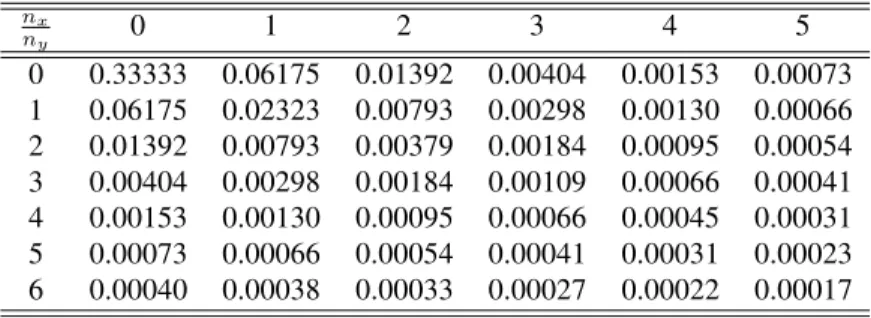
Table 3: Values ofα’s on the planez= 0, for pairs of(nx, ny). nx
ny 0 1 2 3 4 5
0 0.33333 0.06175 0.01392 0.00404 0.00153 0.00073 1 0.06175 0.02323 0.00793 0.00298 0.00130 0.00066 2 0.01392 0.00793 0.00379 0.00184 0.00095 0.00054 3 0.00404 0.00298 0.00184 0.00109 0.00066 0.00041 4 0.00153 0.00130 0.00095 0.00066 0.00045 0.00031 5 0.00073 0.00066 0.00054 0.00041 0.00031 0.00023 6 0.00040 0.00038 0.00033 0.00027 0.00022 0.00017
References
[1] H. Takayasu, Phys. Rev. Lett.54, 1099 (1985). [2] J.C. Dyre. and Th. Schroder B, Rev. of Modern Phys.
72, 873 (2000).
[3] A. Hansen, E.L. Hinrichsen and S. Roux, Phys. Rev. B
[4] V.K.S. Shante and S. Kirkpatric, Adv. Phys.
20, 325 (1971).
[5] M. Sahimi and J.D. Goddard, Phys. Rev. B
32, 1869 (1985).
[6] J.W. Chung, A. Ross, J. Th. De Hosson and E van der Giessen, Phys. Rev. B 54, 15094 (1996-I).
[7] P. Ray and B.K. Chakrabarti, Phys. Rev. B
38, 715 (1988).
[8] Y. Kantor and I. Webman, Phys. Rev. Lett.
52, 1891 (1984).
[9] H.J. Herrmann, A. Hansen and S. Roux, Phys. Rev. B39, 637 (1989).
[10] B.K. Chakrabarti and L.G. Benguigui, “Statistical Physics of Fracture and Breakdown ind Disordered Systems”, Oxford University Press, Inc. N. Y., 1997.
[11] P.M. Duxbury, P.D. Beale and P.L. Leath, Phys. Rev. Lett 57, 1052 (1986) and in Phys. Rev. B
36, 367 (1986).
[12] S. Kirkpatric, Rev. of Modern Phys. 45, 574 (1973). [13] J. Bernasconi, Phys. Rev. B 9, 4575 (1974).
[14] D.G. Harlow and S.L. Phoenix, Int. J. Frac.
17, 601 (1981).
[15] J.S.Espinoza Or-tiz ,Chamith S. Rajapakse, and Gemunu H.Gunaratne, Phys. Rev. B.66, 144203 (2002) and in Virtual Journal of Biological Physics Research-Multicellular Phenom-ena4, issue 9, (2002).
[16] G.H. Gunaratne, C.S. Rajapakse, K.E. Bassler, K.K. Mohanty and S.J. Wimalawansa, Phys. Rev. Lett.