Non-Twist Field Line Mappings for Tokamaks with
Reversed Magnetic Shear
M. Roberto
1, E. C. da Silva
2, I. L. Caldas
2, and R. L. Viana
3 1. Instituto Tecnol´ogico de Aeron´autica, Centro T´ecnico Aeroespacial,Departamento de F´ısica, 12228-900, S˜ao Jos´e dos Campos, SP, Brazil
2. Instituto de F´ısica, Universidade de S˜ao Paulo, 05315-970, S˜ao Paulo, S˜ao Paulo, Brazil
3. Departamento de F´ısica, Universidade Federal do Paran´a, 81531-990, Curitiba, PR, Brazil
Received on 4 February, 2004; revised version received on 7 June, 2004
The structure of magnetic field lines in a tokamak with reversed magnetic shear is investigated by means of analytically derived area-preserving non-twist Poincar´e maps. The basic configuration is the magnetic field produced by an ergodic limiter, superimposed to the tokamak equilibrium field in suitable coordinates. We consider the cases of one and two resonant modes, focusing on magnetic island dimerization and the formation of a transport barrier in the chaotic layer of field lines.
1
Introduction
The Poincar´e map obtained through considering the inter-sections of the magnetic field line flow - in the equilibrium configuration of a tokamak - with a surface of section, is a nice example of twist map. Since, in the equilibrium MHD approach, magnetic field lines are constrained to lie on flux surfaces, if we use as an action variable any surface label, such as the magnetic flux or even a radial-like coordinate, it turns out that the action variable is constant for succes-sive piercings of the field line with the surface of section. On the other hand, the canonically conjugated angle (which can be a poloidal angle, for example) varies according to the rotational transform of the field lines on that surface. This makes for a twist map, which is the starting point of discrete-time Hamiltonian treatments of magnetic field line structure [1, 2]. In this way, plasma physicists have the sin-gular opportunity of facing abona-fidearea-preserving ca-nonical map, which comes directly from the physical setting of a problem.
One result which comes from the Hamiltonian treatment of field line flow is the creation of a chaotic magnetic field line layer in the plasma due to the interaction between reso-nant perturbing fields and the tokamak equilibrium magnetic field. Here the wordchaosmust be intended in its Lagran-gian sense: two field lines, very close to each other, depart exponentially as we follow their revolutions along the toroi-dal chamber. In terms of the field line map, chaos means an area-filling orbit in the surface of section, through which a field line can wander erratically. This affects in a non-trivial way the transport properties of the tokamak plasma, in a way that is only partially understood at present. Field line chaos can be one of the reasons to explain anomalous transport in tokamaks [3].
The presence of chaotic magnetic field lines in a
cer-tain plasma region within the tokamak implies in the loss of the plasma confinement, due to the absence of flux surfa-ces. Thus we could be mislead to conclude that chaos would be necessarily bad to the fusion program. This is not so, however, because the chaotization of a limited plasma re-gion, if properly handled, can be beneficial to the plasma confinement, as exemplified by the ergodic magnetic limi-ter [4]. Another situation in which the presence of magnetic field chaos can help plasma confinement is the creation of a transport barrier to reduce particle escape in tokamaks. It has been recently observed that this may occur if there is a negative magnetic shear region within the plasma column [5, 6]. Such a region is created by means of a non-peaked plasma current density, corresponding to a non-monotonic radial profile for the safety factor [7].
Unlike most area preserving maps used to investigate fi-eld line behavior, negative shear configurations are best des-cribed by non-twist area-preserving maps[8, 9]. Such maps violate the non-degeneracy condition for the Kolmogorov-Arnold-Moser (KAM) theorem to be valid, so that many well-known results of canonical mappings no longer apply to them [10, 11]. For example, it may happen that two neigh-bor island chains approach each other without being des-troyed through the breakup of KAM curves [12]. The trans-port barrier arises from a combination of typical features of non-twist maps: reconnection and bifurcation, occurring in the reversed shear region [13]. This barrier is embedded in a chaotic field line region located in the tokamak periphe-ral region, and which is generated by an ergodic magnetic limiter [14].
to numerically evidence the formation of a transport barrier
0.00 0.10 0.20 0.30 0.40 0.50
R (m) −0.25
−0.15 −0.05 0.05 0.15 0.25
Z (m) θt=0,00
rt=0,14
rt=0,10
θt=π/2
Figure 1. (a) Basic geometry of the tokamak; (b) Scheme of an ergodic magnetic limiter.
barrier due to a reconnection-bifurcation mechanism, and its effect on the plasma transport can be inferred from the study of field line diffusion by using the obtained map. Since the chaotic region generated by a limiter reaches the tokamak wall, the transport barrier we obtain is effective for a limited time-span, such that field lines are eventually lost due to ra-dial diffusion and eventual collision with the wall. However, as a consequence of island reconnection and bifurcation, fi-eld lines are effectively trapped due to the stickiness effect of the magnetic islands, provided the duration of a discharge is less than the average escape time.
The rest of this paper is organized as follows: in section II we present the equilibrium and perturbing equilibrium fi-elds. Section III shows the area-preserving non-twist map obtained for one and two resonant perturbations, and the field line behavior involving reconnection and bifurcation processes. Our conclusions are left to the last section.
2
Equilibrium and perturbing
mag-netic fields
We will use a suitable coordinate systems to describe mag-netic field line geometry in a tokamak:(rt, θt, ϕt), given by [15]
rt=
R′
0
coshξ−cosω, (1)
θt=π−ω, ϕt= Φ, (2)
in terms of the more familiar toroidal coordinates(ξ, ω,Φ). The meaning of these variables is the following: rtis rela-ted to the radial coordinate of a field line with respect to the magnetic axis, which is a circle with radiusR′
0(Fig. 1(a)).
θt andϕtare the poloidal and toroidal angles of this field line, respectively,
The tokamak equilibrium magnetic field B0 = (B0
rt, B
0
θt, B
0
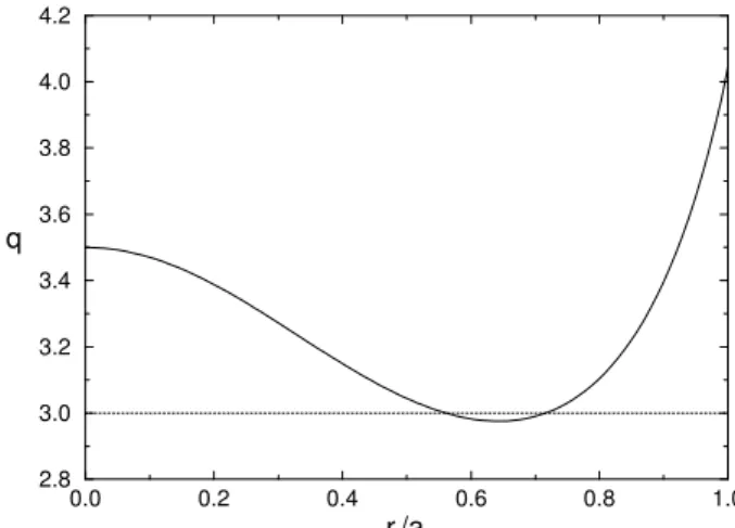
ϕt) is obtained from an approximated analy-tical solution of the equilibrium magneto-hydro-dynamical equation in these coordinates [16]. In order to generate the reversed shear region we have considered a toroidal current density profile with a central hole [17]. There results that the safety factor of the magnetic surfaces, defined as [18]
q(rt) =
1 2π
2π
0 B0
ϕt(rt, θt)
B0
θt(rt)
dθt, (3)
has a non-monotonic profile. For some values of the safety factor there are two magnetic surfaces with different radii within the plasma column with radiusa[17] [see Fig. 2].
0.0 0.2 0.4 0.6 0.8 1.0
rt/a
2.8 3.0 3.2 3.4 3.6 3.8 4.0 4.2
q
The ergodic magnetic limiter consists of Nr current rings of lengthℓlocated symmetrically along the toroidal di-rection of the tokamak [Fig. 1(b)]. These current rings may be regarded as slices of a pair of external helical windings located atrt=b, conducting a currentIhin opposite senses for adjacent conductors. The role of these windings is to in-duce a resonant perturbation in the tokamak, and to achieve this effect we must choose a helical winding with the same pitch as the field lines in the rational surface we want to per-turb. This has been carried out by choosing the following winding law [16]ut=m0θt−n0ϕt=constant. In this pa-per we will consider an ergodic limiter consisting ofNr= 4 rings with mode numbers(m0, n0) = (3,1)each, carrying
a currentIh.
The magnetic fieldB1
produced by the resonant helical winding, from which we build the EML rings, is obtained by neglecting the plasma response and the penetration time th-rough the tokamak wall. We were able to obtain an approxi-mated analytical solution in lowest order for the limiter field, through solving the corresponding boundary value problem. The model field to be used in this paper will be the superpo-sition of the equilibrium and limiter fields: B=B0+
B1
.
Since the equilibrium field is axisymmetric, we may set the azimuthal angle,ϕt=t, as a time-like variable, and put the magnetic field line equations in a Hamiltonian form
[19]
dJ
dt = −
∂H
∂ϑ, (4)
dϑ
dt =
∂H
∂J, (5)
where(J, ϑ)are the action-angle variables of a Hamiltonian
H, its explicit form being given in Ref. [20]. In that paper we analyzed exact but numerically obtained maps, whereas in this work we derive analytical, albeit approximate, forms of these maps.
The addition of the magnetic field produced by a reso-nant helical winding may be regarded as a Hamiltonian per-turbation. In order to include the effect of the finite lengthℓ
of each EML ring, which is typically a small fraction of the total toroidal circumference2πR′
0, we model its effect as a
sequence of delta-functions centered at each ring position. The Hamiltonian for the system is thus
⌋
H(J, ϑ, t) =H0(J) + ℓ R′
0
H1(J, ϑ, t) +∞
k=−∞
δ
t−k2π Nr
, (6)
We consider the perturbing Hamiltonian as a periodic function in bothϑandtvariables, such that it can be written as a Fourier series in these variables. There results a model Hamiltonian
H(J, ϑ, t) =H0(J) +ǫ 2m0
m=0 H∗
m(J) cos(mϑ−n0t) +∞
k=−∞
δ
t−k2π Nr
, (7)
⌈
where H∗
m are Fourier coefficients, whose detailed forms can be found in Ref. [20], and the perturbation strength is expressed by the parameter
ǫ=−2
ℓ 2πR′
0 Ih
Ie
, (8)
which is usually small, since in experiments we have
ℓ ≪ 2πR′
0 andIh ≪ Ie, whereIe is the coil current producing the toroidal equilibrium field.
3
Non-twist maps for one and two
re-sonant modes
The non-monotonicity of the radial safety factor profile ma-kes possible to have two resonant surfaces with the same value of the safety factor. From the Hamiltonian theory of
quasi-integrable systems we know that there appear two is-land chains centered at these radii. A periodic isis-land results from the resonance between the equilibrium tokamak field and one mode of the perturbation field. Let us suppose that we are dealing with a resonant perturbation with (positive integer) mode numbers(m0, n0), such that the safety factor m0/n0 is a rational number. In terms of the action-angle
variables of the unperturbed Hamiltonian, corresponding to the tokamak equilibrium field, this is a frequency, which is the same for the two island chains centered atJ∗
1 andJ
∗
2
ω0(J
∗
1) =ω0(J
∗
2) = ∂H0
∂J =
n0 m0
. (9)
The dynamical behavior in the vicinity of the resonant surfaces located atJ∗
1 andJ
∗
2 can be investigated by
pic-king up from the model Hamiltonian, Eq. (7), the resonant term corresponding to the frequencyn0/m0:
⌋
H(J, ϑ, t) =H0(J) +ǫH
∗
m0(J) cos(m0ϑ−n0t)
+∞
k=−∞
δ
t−k2π Nr
and expanding the Hamiltonian in the neighborhood of the rational surface beyond the cubic approximation. This is actually necessary for taking into account the fact that the unperturbed HamiltonianH0fails to satisfy KAM theorem,
due to the non-monotonicity of the frequency. As a
conse-quence, the island chains are not pendular (i.e., their widths do not increase as the square root ofǫ), and we need a higher order approximation in order to capture the essentials of the twins islands’ behavior.
After dropping the constant terms, we obtain
⌋
H(∆J, ϑ, t) ≈ ω0(J
∗
)∆J +1
2 dω0 dJ J=J∗
(∆J)2+1 6
d2ω 0
dJ2 J=J∗
(∆J)3+· · ·
+ ǫH∗
m0(J ∗
) cos(m0ϑ−n0t) +∞
k=−∞
δ
t−k2π Nr
, (11)
⌈
where∆J =J − J∗ .
We can simplify this expression by performing a cano-nical transformation to new action-angle variables(J′, ϑ′) which eliminates the explicit time-dependence, what can be done through the generating function
S(J′
, ϑ, t) =
ϑ− n0
m0 t
J′
, (12)
leading to the local Hamiltonian
H′(J′, ϑ′) = M
2 J
′2
−W
3 J
′3
+Kcos(m0ϑ
′
) +∞
k=−∞
δ
t−k2π Nr
, (13)
in which we have defined
M(J∗
) ≡ dω0
dJ J=J∗
, (14)
W(J∗
) ≡ 1
2 d2ω
0
dJ2 J
=J∗
, (15)
K(J∗
) ≡ ǫH∗
m0(J ∗
1,2). (16)
After dividing both sides of Eq. (13) by M, what amounts to re-scale the field line Hamiltonian, we have
H(J′
, ϑ′
) =1
2J
′2
−α
3J
′3
+κcos(m0ϑ
′
) +∞
k=−∞
δ
t−k2π Nr
, (17)
whereα=W/Mandκ=K/M.
In theα = 0 limit, the Hamiltonian above reduces to that of a nonlinear pendulum, which is the standard proce-dure used in perturbation theory to describe the phase-space structure near a given resonance [2]. Hence,αmeasures, so as to speak, the non-pendular character of the island chains. The corresponding Hamilton equations are
dJ′
dt = m0κsin(m0ϑ
′
) +∞
k=−∞
δ
t−k2π Nr
, (18)
dϑ′
dt = J
′
(1−αJ′
). (19)
Writing down the summation in t as a Fourier series and isolating the resonant term, we can use these equations to predict the widths of each non-pendular island as well as to make an estimation of the critical value of the limiter current necessary to their reconnection [20].
The fact that the “time”-dependence of the Hamilton equations is in the form of a periodic sequence of delta func-tion kicks enables us to define discretized variables [21]
ϑ′
k = lim ǫ→0ϑ
′
(t=tk+ǫ) (20)
J′
k = lim ǫ→0J
′
(t=tk+ǫ) (21)
as the angle and action, respectively, just after the k-th kick, which occurs at timetk = k(2π/Nr)(note that one Poin-car´e section of the field line flow is done afterNrm0turns
around the torus, rather than simply sampling out the field line position after each turn, as usually done). The resulting field line map is thus
J′
k+1 = J
′
k+m0κsin(m0ϑ
′
k+1), (22)
tk+1 = tk+
2π Nr
, (23)
ϑ′
k+1 = ϑ
′ k+
2π Nr
J′
k(1−αJ ′
k) (mod2π).(24)
If we switch off the perturbation(κ= 0), the map above reduces to a simple non-twist map, for which all trajecto-ries are bound to invariant tori with constantJ′
. The non-monotonic character of the equilibrium field is expressed in theαterm which appears in the winding number term in Eq. 24. From now on we choose an ergodic limiter withNr= 4 rings, uniformly spaced from each other along the tokamak torus (i.e. with angular separationπ/2), each of them with
m0= 3pairs of wires. The plasma current density profile is
supposed to yield a non-monotonic profile for the winding numberω=∂H0(J′)/∂J′, such that there are two values
of the action variable forω= 1/3.
If we pick up two resonant modes from the model Hamiltonian (7), there will appear terms in cos[m0ϑ′ − (n0/m0)t]andcos[(m0+ 1)ϑ′−(n0/m0)t]. The derivation
J′
k+1 = J
′
k+m0κsin(m0ϑ′k+1) + (m0+ 1)˜κsin
(m0+ 1)ϑ′k+1
, (25)
ϑ′
k+1 = ϑ
′ k+
2π Nr
J′
k(1−αJ ′
k) (mod2π) (26)
tk+1 = tk+
2π Nr
, (27)
⌈
whereκ˜ = κ1Ih,κ1 being the amplitude of the second
re-sonant mode. The map is obtained for eachm0turns around
the tokamak torus.
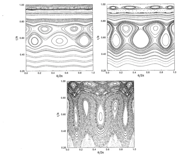
For small limiter currents [Fig. 3(a)] we have: (i) two chains of non-pendular islands centered at the points J∗
1
andJ∗
2, due to the non-monotonic character of the safety
factor profile [see Fig. 2]; (ii) a third chain of pendular islands centered at the position of the second resonance
(m0+ 1)/n0 = 4/1, since for this value ofqwe have just
one resonant surface, according to Fig. 2.
In the region of reversed magnetic shear, due to the lo-cally KAM nature of the Hamiltonian, the map is non-twist. Hence, the two non-pendular islands of the3/1-chain can approach each other without destruction of tori. For a perturbation strong enough [Fig. 3(b)] the island chains di-merize, forming a unique sequence of islands which share a common separatrix. This is called reconnection, but it is rather a topological effect, involving no dissipative breakup and re-wiring of the field lines, as it occurs in astrophysical and fusion situations. After the reconnection takes place we find curves (meanders) which encircle both sets of islands, forming a unique path which will be the foundation of the transport barrier to be described.
The action of an ergodic limiter actually produces an in-finite number of resonant modes due to the localized nature of the generated fields in the toroidal direction (note the infi-nite terms in the summation in Eq.(17), for example). Since the magnetic field generated by a magnetic limiter falls off rapidly as we move apart from the tokamak wall [16], the amplitudes of the corresponding resonant modes also decre-ase as we go into the tokamak center. Hence, the main reso-nance is just that produced near the tokamak wall, the others having exponentially smaller widths.
In fact, as the limiter currentIhincreases, all mode am-plitudes are augmented, yet not in the same proportion. For many purposes these higher modes are not important and hence it suffices to pick up just one resonant mode from the field line Hamiltonian (17). However, in order to study the formation of a large chaotic region inside the tokamak plasma, it is necessary to take into account a second resonant mode from the infinite number of possible modes. Since this second chain is now pendular, they will not dimerize with the first resonant mode. As the perturbation strength increa-ses both islands become wider and they interact as predicted by the global stochasticity mechanisms widely studied in the literature [Fig. 3(c)] [2].
As the limiter current increases further [Fig. 3(c)] we can see that: (a) the twin chains of the first mode have already dimerized and suffered reconnection, with open surfaces ex-ploring the former twin chains (this is actually necessary for the transport barrier be present); and (b) there are visible chaotic layers surrounding both sets of islands. However, as the limiter current is still not high enough, there are many surviving invariant curves between the sets of islands. This is, in fact, a result from KAM theorem which applies here because this region has a monotonic frequency profile and, at least locally, the conditions for the KAM theorem to be valid are fulfilled.
Even higher limiter currents will destroy entirely the in-variant curves between both chains and a wide chaotic layer appears surrounding both modes. At least in principle, Chi-rikov’s criterion for global stochasticity applies in this case and predicts the formation of such layer [1]. The transport barrier appears embedded in this large chaotic layer and is structured around the path of open curves which encir-cled the formerly dimerized islands after reconnection. This layer acts as an effective transport barrier since it hampers the radial diffusion of field lines, and arises from the “stic-kiness” effect that the region near the former separatrices of islands exert on the chaotic trajectories. This effect has been related to manifold reconnection in Ref. [13] occurring in-side the chaotic region. This barrier is effective provided the duration of a typical tokamak plasma discharge is less than the average escape time.
4
Conclusions
Figure 3. Poincar´e maps (in scaled toroidal coordinates) for two resonant modes with (a)κ0=−6.33101×10⁻⁶,κ1= 2.91385×10⁻⁶;
(b)κ0=−1.477235×10⁻⁵,κ1= 6.798983×10⁻⁶; (c)κ0=−8.441344×10⁻⁵,κ1= 3.885133×10⁻⁵.
This layer works like an effective transport barrier, with respect to the typical plasma duration. The trapping is more intense around the shearless plasma, and results from the properties of field line trajectories in the vicinity of separa-trices of islands bordering the chaotic region. This transport barrier can help plasma confinement preventing energetic charged particles from escaping out radially to an eventual collision with the tokamak inner wall.
Acknowledgments
This work was made possible with partial financial sup-port of the following agencies: CNPq and FAPESP.
References
[1] B. Chirikov, Phys. Reports (1979)
[2] A. J. Lichtenberg and M. A. Lieberman,Regular and Chaotic Dynamics, 2nd. Edition (Springer-Verlag, New York-Berlin-Heidelberg, 1992).
[3] J. D. Meiss, Rev. Mod. Phys.64, 796 (1992). Neoclassical transport, (North Holland Publ., Amsterdam, 1988).
[4] J. E. S. Portela, R. L. Viana, and I. L. Caldas, Physica A317, 411 (2003).
[5] F. M. Levinton, M. C. Zarnstoff, S. H. Batha, et al., Phys. Rev. Lett.75, 4417 (1995).
[6] E. J. Strait, L. L. Lao, M. E. Manel,et al., Phys. Rev. Lett.
75, 4421 (1995).
[7] E. Mazzucato, S. H. Batha, M. Beer,et al., Phys. Rev. Lett.
77, 3145 (1996).
[8] P. J. Morrison, Phys. Plas.7, 2279 (2000).
[9] R. Balescu, Phys. Rev. E58, 3781 (1998).
[10] D. Castillo-Negrete, J. M. Greene, and P. J. Morrison, Phy-sica D91, 1 (1996).
[11] E. Petrisor, J. H. Misguich, and D. Constantinescu, Chaos, Solit. & Fract.18, 1085 (2003).
[12] J. E. Howard and S. M. Hohs, Phys. Rev. A29, 418 (1984).
[13] G. Corso, F. B. Rizzato, Phys. Rev. E58, 8013 (1998).
[14] E. C. da Silva, I. L. Caldas, and R. L. Viana, Phys. Plasmas
8, 2855 (2001); Chaos, Solit. & Fract.14, 403 (2002).
[16] E. C. da Silva, I. L. Caldas, and R. L. Viana, IEEE Trans. Plas. Sci.29, 617 (2001).
[17] G. A. Oda and I. L. Caldas, Chaos, Solit. & Fract. 5, 15 (1995); G. Corso, G. A. Oda, and I. L. Caldas, Chaos, So-lit. & Fract.8, 1891 (1997).
[18] J. Wesson,Tokamaks(Oxford University Press, 1987).
[19] I. L. Caldas, R. L. Viana, M. S. T. Araujo,et al., Braz. J. Phys.
32, 980 (2002).
[20] M. Roberto, E. C. da Silva, I. L. Caldas, and R. L. Viana, Phys. Plasmas11, 214 (2004).