Bounds on functionals of the distribution treatment effects

Bounds on Functionals of the Distribution

of

Treatment Effects

S

ERGIO

F

IRPO

G

EERT

R

IDDER

Setembro

de 2008

T

T

e

e

x

x

t

t

o

o

s

s

p

p

a

a

r

r

a

a

D

D

i

i

s

s

c

c

u

u

s

s

s

s

ã

ã

o

o

T

D

201

•

2008

•

1

Os artigos dos

Textos para Discussão da Escola de Economia de São Paulo da Fundação Getulio

Vargas

são de inteira responsabilidade dos autores e não refletem necessariamente a opinião da

FGV-EESP. É permitida a reprodução total ou parcial dos artigos, desde que creditada a fonte.

Escola de Economia de São Paulo da Fundação Getulio Vargas FGV-EESP

Bounds on Functionals of the Distribution of

Treatment Effects

∗

Sergio Firpo

Escola de Economia de S˜

ao Paulo, FGV-Brazil

Geert Ridder

Department of Economics, University of Southern California

September 22, 2008

Abstract

Bounds on the distribution function of the sum of two random vari-ables with known marginal distributions obtained by Makarov (1981) can be used to bound the cumulative distribution function (c.d.f.) of indi-vidual treatment effects. Identification of the distribution of indiindi-vidual treatment effects is important for policy purposes if we are interested in functionals of that distribution, such as the proportion of individuals who gain from the treatment and the expected gain from the treatment for these individuals. Makarov bounds on the c.d.f. of the individual treat-ment effect distribution are pointwise sharp, i.e. they cannot be improved in any single point of the distribution. We show that the Makarov bounds are not uniformly sharp. Specifically, we show that the Makarov bounds on the region that contains the c.d.f. of the treatment effect distribution in two (or more) points can be improved, and we derive the smallest set for the c.d.f. of the treatment effect distribution in two (or more) points. An implication is that the Makarov bounds on a functional of the c.d.f. of the individual treatment effect distribution are not best possible. Keywords: Treatment effects, bounds, social welfare.

JEL-code: C31

∗_{Financial support for this research was generously provided through NSF grant}

SES 0452590 (Ridder) and by CNPq (Firpo). We thank Rustam Ibragimov, Guido Imbens, Yanqin Fan and seminar and conference participants at Harvard Econometrics Lunch, IZA-Bonn, 2007 North American Winter Meeting of the Econometric Society and UFRJ-Brazil for comments.

†_{Rua Itapeva 474, S˜ao Paulo, Brazil, 01332-000. Electronic correspondence:}

ser-gio.firpo@fgv.br.

‡_{Kaprilian Hall, Los Angeles, CA 90089. Electronic correspondence:}

1

Introduction

The key problem when estimating the effect of a treatment or intervention on a population is that we cannot observe both the treated and non-treated out-comes for a unit in the population, but at most either its treated or non-treated outcome. As a consequence, we can only identify treatment effect parameters that depend on the marginal distributions of the treated and control outcomes and, in general, not parameters that depend on the distribution of individual treatment effects. The only exception is the mean of the individual treatment effect distribution, the Average Treatment Effect (ATE), which, given linearity of expectations, can be identified from the marginal distributions of treated and control outcomes.

Under the assumption that the social welfare function (SWF) is a functional of the distribution of outcomes, gains or losses in social welfare due to an in-tervention can be measured as the difference of functionals on the marginal distributions of treated and non-treated outcomes. For instance, we may be interested in the effect of a program on the inequality of outcomes in the pop-ulation. If we choose some inequality measure, say the variance, then the effect of the program on the variance is equal to the difference of the variances of the marginal distributions of the treated and control outcomes. Such an approach has been used, for example, in Imbens and Rubin (1997), Abadie, Angrist Im-bens (2002), Abadie (2002, 2003) and Firpo (2007). Therefore, if our goal is to assess the effect of an intervention on social welfare and not individual welfare, then the marginal outcome distributions suffice.

There are some other treatment effect parameters that are defined as tionals of the distribution of individual treatment effects. Examples of func-tionals of the distribution of individual treatment effects are the fraction of the population that benefits from a program, the total and average gains of those who benefit from the program, the fraction of the population that has gains or losses in a specific range, and the median (or other quantile) of the treatment effect distribution.1 _{Heckman, Smith and Clements (1997) discuss a number of}

parameters that depend on the distribution of individual treatment effects. We show that a general reason why we should be interested in functionals of the distribution of individual treatment effects is that individuals in a pop-ulation may be loss averse. Loss aversion has been shown to be a feature of individual preferences if an individual faces an uncertain outcome (e.g. Tversky and Kahneman (1991) and the large literature on non-expected utility). With loss aversion at the individual level a utilitarian social welfare function will ex-hibit aversion to redistribution. As a consequence the social welfare function depends on the distribution of individual treatment effects.

Point identification of parameters that depend on the distribution of individ-ual treatment effects requires knowledge of the joint distribution of treated and non-treated outcomes, as the marginal themselves do not contain enough

infor-1

mation to identify the distribution of the difference. If the treatment effect is the same for all members of the population or of subpopulations characterized by a vector of observable variables, this (conditional) joint distribution is singular and the (conditional) distribution of individual treatment effects is degenerate. However, in most cases the observed (conditional) marginal distributions are not related by a simple location shift. In that case we can either introduce addi-tional information that allows us to point identify the distribution of treatment effects, or we can as e.g. Heckman, Smith and Clements (1997) derive bounds on the distribution of treatment effects.

Bounds on the cumulative distribution function (c.d.f.) of the sum of two random variables with known marginal distributions were first obtained by Makarov (1981) and the generalization to the difference is trivial. Fan and Park (2007) were the first to apply these bounds to the distribution of treatment effects with an emphasis on the statistical inference for these bounds.

This paper will disregard inference completely and will focus instead on the nature of the Makarov bounds. An important property of a bound is whether it is sharp or best possible. Our results show that Makarov bounds arepointwise

but not uniformly sharp. This implies that Makarov bounds on functionals of the distribution of individual treatment effects are in general not sharp. In the case of a scalar parameter bounds are defined by a set of restrictions on the parameter. Assume for simplicity that these restrictions imply that the parameter is in a closed connected interval. A lower bound on the parameter is sharp if every parameter value that satisfies the restrictions is not smaller than the bound and the bound itself satisfies all the restrictions. In the case that we bound a function defined on some domain the definition of a sharp bound is not as simple. Again the bounds are defined by a set of restrictions. In our case we consider all c.d.f. of a distribution ofY1−Y0whereY0, Y1have a

joint distribution with given marginal distributions. If the bounding functions satisfy all the restrictions we call them uniformly sharp. This corresponds to the usual definition of sharpness for a scalar parameter. The Fr´echet (1951) (see also Hoeffding (1940)) bounds on the joint distribution of two random variables with given marginal distributions are uniformly sharp. It is however possible that the bounding functions do not satisfy all the restrictions. This is the case with the Makarov bounds. In that case it is possible that the bounds are best possible in a point (and every point) of the domain. This occurs if there is a function that satisfies all the restrictions and is equal to the bounding function at that point (and such a function exists at every point)2. We call such a bound pointwise sharp. The Makarov bounds are pointwise, but not uniformly sharp. If a bound is uniformly sharp, then the joint bound on the set of function values in two (or more) points on the domain derived from the uniformly sharp bound and possible other restrictions like monotonicity is also sharp. This is not true if the bounds are pointwise sharp.

In this paper, we show that a joint bound of c.d.f. points using the Makarov bounds is not best possible. Moreover, we derive more informative joint bounds,

2

i.e. a smaller region, for the c.d.f. of the individual treatment effect in two (or more) points. This result is not at odds with the sharpness of the Makarov bounds in a single point, because the projections of the smaller higher-dimensional region coincides with the one-dimensional Makarov bounds. Bounds on the treatment effect c.d.f. in two (or more) points imply bounds on functions of the treatment effect c.d.f in those points. We consider linear functionals of the treatment effect c.d.f. and derive conditions under which the bounds on this functional can be improved.

A second contribution of this paper is that we show that if the outcomes are correlated with covariates, then averaging the bounds obtained from the condi-tional (on these covariates) outcome distributions gives bounds that are more informative than the bounds obtained from the unconditional outcome distribu-tions. This result holds both for the one-dimensional pointwise Makarov bounds and for the improved higher dimensional regions. Hence, even if treatment is randomly assigned it is useful to have covariates that are correlated with the outcomes in order to improve the bounds on (functionals of) the distribution of the individual treatment effects.

There is a small literature on bounds on the treatment effect c.d.f. in a point for given marginal outcome distributions. None of it considers bounds on the c.d.f. in two or more points or bounds on functionals of the c.d.f. We already mentioned Fan and Park (2007) who use the pointwise sharp Makarov bounds. Most papers introduce additional restrictions, as a factor structure or rank preservation that narrow the bounds or even lead to point identification of the treatment effect distribution. In chronological order contributions can be found in Heckman and Smith (1993, 1998) and in particular Heckman, Smith and Clements (1997), Aakvik, Heckman and Vytlacil (2005), Carneiro, Hansen and Heckman (2003), and Wu and Perloff (2006). Djebbari and Smith (2008) use the Heckman-Smith-Clements bounds3_{in an empirical study of the distribution}

of treatment effects in a conditional cash transfer program in Mexico.

The plan of he paper is as follows. In section 2 we show that if individuals are loss averse then the social welfare function is a functional of the distribution of individual treatment effects. In section 3 we discuss the Makarov bounds on the cdf of treatment effects and we introduce the concepts of pointwise and uniformly sharp bounds. Section 4 establishes that the Makarov bounds are pointwise, but in general not uniformly sharp. In section 5 we show that averaging over covariates that are correlated with the outcomes improves the bounds. In section 6 we obtain higher dimensional Makarov bounds and we derive a necessary condition for a vector of function values to be compatible with a treatment effect distribution. We then use this necessary condition to show that the higher dimensional Makarov bounds are in general not sharp and we derive improved bounds. In section 7 we use these improved bounds to obtain improved bounds on functionals of the treatment effect distribution. Section 8 concludes.

3

2

Welfare and the distribution of treatment

ef-fects

Consider an intervention with potential outcomes Y0i and Y1i for individual i of the population. The individual has a vector of characteristics Xi. An

experiment is performed in a randomly selected sample from this population and treatment assignmentTi in the sample is either random or unconfounded

givenX. Hence, if the sample is large we can identifyF0(.|x) andF1(.|x) for all

x∈ X withX the support of the distribution ofX. Let us defineDi=Y1i−Y0i

and assume that alli know Y0i, their non-treated or status quo outcome, but

not necessarilyY1i, their treated outcome at the time of treatment. In general Y1i can be thought of as a function of Xi and εi, where Xi is a vector of

characteristics that is known to the individual and εi is a random term that

may or may not be known to individualiat the time of the intervention. We assume thatY0i is known to the individual at the time of the intervention even

ifiundergoes the intervention. Ifiundergoes the intervention, then Y0i is not

known to the econometrician or the social planner. The vectorXi is observed

irrespective of treatment assignment (and not affected by that).

Note that the treated and control outcomes are treated asymmetrically. Of-ten individuals can predict their outcome under the status quo accurately but not necessarily their outcome under the treatment. We consider both the case thatY1i is known at the time of the treatment and the case that this outcome

is not known at that time. Moreover, we consider two types of preferences. The first type corresponds to expected utility in the case that Y1i is unknown toi

at the time of the treatment. The second type assumes that individuals are loss averse, as introduced by Tversky and Kahneman (1991) and extensively discussed by Rabin (1998). For the second type of preferences we need the dis-tribution ofD at the time of treatment. We also consider the utilitarian social welfare functions corresponding to these individual preferences.

The social welfare functions are our main focus in this section. They are the same irrespective which assumption we make on knowledge of Y1 at the time

of treatment (we consider the unknownY1case only for expositional purposes).

If we start from individual preferences that exhibit loss aversion we obtain a social welfare function that has redistribution aversion. In particular, if we fix the average benefit of an intervention, i.e. the Average Treatment Effect (ATE), then society will prefer an intervention that spreads the gains evenly in the population over an intervention that achieves the same ATE with large losses for some and slightly larger gains for others in the population. Easterlin (2008) discusses the relevance of the distribution of gains and losses for social welfare in a transition economy.

First, we assume thatY1i is not known (but Y0i is) toi at the time of the

treatment. Both outcomes are net of the private cost of treatment and non-treatment. If the utility of outcomeY isu(Y) withuconcave ifiis risk averse, then the expected utility of treatment foriisE_[u(Y1i)|Y0i, Xi] and the expected

individual preferences over all members of the population is

W1=E[E[u(Y1)|Y0, X]] =E[u(Y1)]

and

W0=E[u(Y0)]

Both individual and social welfare only depend on the marginal distributions of Y0 and Y1 (given X). If we assume that both Y0i and Y1i are known to i at the time of treatment then the individual utilities of treatment and non-treatment areu(Y0i) and u(Y1i), respectively. Therefore, the utilitarian social

welfare function assignsW1andW0to treatment and non-treatment, which are

the same values as in the case thatY1i is not known at the time of treatment.

The obvious conclusion is that utilitarian social welfare depends only on the marginal outcome distributions and the distribution ofD does not play a role4_.

As Tversky and Kahneman (1991) have pointed out, individual preferences are actually not as in the standard expected utility theory. In (cumulative) prospect theory preferences exhibit the so-called “framing effect”, because peo-ple tend to think of possible outcomes relative to a reference value. In the simple potential outcome model the natural choice for the reference value is the status quo outcome Y0i. Moreover, individuals have different risk

atti-tudes towards gains Y1i −Y0i > 0 and losses Y1i −Y0i < 0 and the

disutil-ity of a loss is in general larger than the utildisutil-ity of an equal gain. This is called loss aversion. If we denote the valuation function of gains/losses by

v(Y1−Y0) = v+(Y1−Y0)1(Y1−Y0 > 0) +v−(Y1−Y0)1(Y1−Y0 ≤ 0) then

the utility of non-treatment is 0 (essentially a normalization) and the utility of treatment is5

E_v+_{(Y1i−Y0i)1(Y1i−Y0i>0)|Y0i, Xi+}E_v−

(Y1i−Y0i)1(Y1i−Y0i≤0)|Y0i, Xi

.

Hence the utilitarian social welfare isV0= 0 and

V1=E

v+(Y1−Y0)1(Y1−Y0>0)

+E_v−

(Y1−Y0)1(Y1−Y0≤0)

.

Two interesting particular cases of valuation functions are the following. If

v+_(Y

1−Y0) = 1 andv−(Y1−Y0) =−1 thenV1is the difference of the fractions

of the population with a positive and a negative treatment effect respectively. This majority parameter is mentioned by Heckman, Smith and Clements (1997). If

v+_(Y

1−Y0) =v−(Y1−Y0) =u(Y1)−u(Y0),

then the expected utility and loss aversion social welfare functions are the same (up to normalization).

In general, the valuation functions are such thatv+_{(0) =v}−

(0) = 0,v+_(z)≥

0 for z ≥ 0, v−

(z) ≤ 0 for z < 0, and v+_{(z) < −v}−

(−z), where the final

4

We could also let the utility function depend onX, i.e., consideru(Y, X). In that case knowledge of the conditional distributions ofY0 andY1givenX is sufficient.

5

condition is loss aversion. Also, it is often assumed thatv+ _{is concave andv}− is convex, and both are increasing inz.

Now, suppose we want compare two possible treatments, A and B. Both treatments have the same ATE,E_[Y1]−E_{[Y0]. However, for treatment Aevery}

individual has a gain equal to the ATE and for treatmentB some individuals have a large loss while an equal fraction of the population has a gain that exceeds the (opposite of the) loss by the ATE. It is obvious that treatmentAis preferred over treatmentB if individuals are loss averse. TreatmentAdoes not involve any redistribution of gains while under treatmentBgains and losses are unequal. Therefore we can say that a social welfare function derived from loss averse individual preferences showsredistribution aversion.

The loss aversion social welfare function is also relevant if individual treat-ment effects are nonnegative, i.e. if all individuals benefit from the treattreat-ment. Individuals may still use the status quo outcome as a reference. As a conse-quence, society may prefer less variation in the distribution of individual gains. Although we derived the social welfare function on the assumption that individuals use the known non-treated outcome as a reference, the analysis is also relevant in the case that treated individuals only learnY1 (so that the reference

value is unknown) and control individuals only learnY0. Let us first assume

that the identifiedF0 andF1are known. For individuals who are in the control

group the expected utility under loss aversion is as above (the expectation is over F1). For individuals who are treated the expected utility is of the same

form except that the expectation is overF0. The social welfare function does not

change. If individuals only learnY0or Y1 and not their marginal distributions,

then the social planner may still care about the distribution of gains and use the redistribution averse social welfare function. Of course, because onlyF0andF1

are identified the social planner can only prefer treatmentAover treatmentB

if the lower bound on the social welfare ofA exceeds the upper bound on the social welfare ofB. If the bounds overlap the social planner has to use some criterion to rank the treatments, e.g. the largest lower bound.

The social welfare function that assumes that individual preferences exhibit loss aversion depends in general on the distribution of the individual treatment effectD. By partial integration we find

V1=

Z ∞

0

v+′

(z)·(1−G(z))dz−

Z 0

−∞

v−′

(z)·G(z)dz

wherev+′ (z),v−′

(z) are the derivatives ofv+_(z),v−

(z) andGis the cdf ofD. As noted, the functionsv+_andv−

are in general nonlinear increasing functions. An obvious specification is a linear spline with nodes 0 =d0< d1< . . . < dK=∞

andv+₀ = 0,vk+>0

v+(z) =

K

X

k=1

[vk+(z−dk−1) +vk+−1dk]1(dk−1≤z < dk)

and a similar specification forv−

andv−

are step functions so that

Z ∞

0

v+′(z)(1−G(z))dz=

K

X

k=1

v+k

Z dk

dk₋1

(1−G(z))dz

In section 7 we consider bounds on integralsRdk

dk₋1(1−G(z))dz.

3

Pointwise and uniformly sharp bounds on the

distribution of treatment effects

LetG be a set of distribution functions on ℜ, i.e. a set of non-decreasing and right-continuous functions onℜthat are 0 in−∞and 1 in∞. All distribution functions inG satisfy a set of restrictions. In this paper the restriction is that eachG ∈ G is the c.d.f. of D =Y1−Y0 for given marginal c.d.f. of Y1,

de-noted byF1, andY0, denoted byF0, but unspecified joint distribution ofY0, Y1.

We are interested in bounds on the distribution functions in G, which is the set of distributions of individual treatment effects for given marginal outcome distributions. We often have a vector of covariatesX with a distribution with supportX that are correlated withY1andY0, so that in the statement above we

can replace the treatment effect distribution by the conditional treatment effect distribution givenX and the outcome distributions by conditional outcome dis-tributions. The bounds on the distribution of the treatment effect are obtained by averaging the conditional bounds over the distribution ofX. Sometimes it is convenient to ignore the fact that we are dealing with conditional distributions and only to introduce the covariates in the final result. In general, averaging makes the bounds more informative.

An upper and lower bound onG(d) forG∈ Gwas derived by Makarov (1981) (see also Frank, Nelsen, and Schweizer, 1987). Note that this is a bound for the c.d.f. in a single point. We extend the Makarov bound to the case that we observe conditional marginal distributions of the outcomesF0(.|x) andF1(.|x).

Theorem 3.1 (Makarov, 1981) Let the conditional c.d.f. ofY0|X andY1|X be F0(.|X) and F1(.|X) and G ∈ G be the c.d.f. of D = Y1−Y0, then for

−∞< d <∞

GM L(d)≡E

sup

t

max{F1(t|X)−F0(t−d|X)−,0}

≤G(d)≤

Eh_inf

t min{F1(t|X)−F0(t−d|X)−+ 1,1}

i

≡GM U(d)

(1)

withF0(.)−the function of left-hand limits of the c.d.f.. The boundsGM L(d), GM U(d)

are c.d.f., i.e. non-decreasing, right-continuous, and 0 and 1 for d↓ −∞ and

Proof:See Appendix B.

Are the Makarov bounds on the treatment effect c.d.f. the best possible bounds? The answer to this question depends on our definition of best possible bounds. Because we are bounding a function we can consider bounds in each point d or joint bounds for all d. If we consider bounds in a single point d, then the relevant notion is pointwise sharpness. To keep the notation simple the discussion is for unconditional c.d.f. but it applies directly to conditional c.d.f.

Definition 3.1 (Pointwise sharp bounds on a c.d.f.) LetGbe a set of c.d.f. and letGL(d)≤G(d)≤GU(d) for alld∈ ℜand G∈ G. We say that GL is a

pointwise sharp lower bound onG, if for all d0 there is a c.d.f. Gd0L ∈ G such that GL(d0) =Gd0L(d0). GU is a pointwise sharp upper bound on G, if for all

d0 there is a c.d.f. Gd0U ∈ G such thatGU(d0) =Gd0U(d0). 6

Note that the c.d.f. that supports the lower bound may depend on d0. If

for alld0 the supporting c.d.f. does not depend ond0 we call the lower bound uniformly sharp. A uniformly sharp upper bound is defined analogously.

Definition 3.2 (Uniformly sharp bounds on a c.d.f.) LetGbe a set of c.d.f. and letGL(d)≤G(d)≤GU(d) for alld∈ ℜand G∈ G. We say that GL is a

uniformly sharp lower bound on G, ifGL∈ G. GU is a uniformly sharp upper

bound onG, ifGU ∈ G.

It should be noted that if the bounds are uniformly sharp they have all the properties of the setG. If they are pointwise sharp, the bounds will have some but not all properties ofG.

Theorem 3.2 If G is a set of c.d.f. with pointwise sharp boundsGL, GU, then GL, GU are non-decreasing, right-continuous and 0 and 1 at −∞ and ∞,

re-spectively, i.e. the bounds are themselves c.d.f.7

Proof:See Appendix B.

4

Makarov bounds are pointwise sharp

We are now able to answer the question whether the Makarov bounds are best possible. Frank, Nelsen, and Schweitzer (FNS) (1981) construct for anyd0joint

distributionsHd0LandHd0U ofY0, Y1such that

GM L(d0) =

Z ∞

−∞ Z v+d0

−∞

dHd0L(u, v) GM U(d0) =

Z ∞

−∞ Z v+d0

−∞

dHd0U(u, v)

6

Although we define these concepts for sets of c.d.f. they apply to any set of functions on

ℜ.

7

i.e. these joint distributions support the lower and upper bounds. It is instruc-tive to show the result of the construction, because it clearly illustrates that the supporting c.d.f. are local, i.e. they depend on d0, so that the Makarov

bounds are pointwise sharp. To keep the notation simple we consider the case that the marginal c.d.f. F0andF1are strictly increasing on the respective

sup-ports. We only consider the supporting c.d.f. Gd0L of the lower Makarov bound

in d0. Instead of the joint c.d.f. of Y1, Y0, Hd0L, we consider that of Y1,−Y0,

˜

Hd0L that has a simpler form. Define u0=F

−1

1 (GM L(d0)) ,v0=d0−u0, and

v1 = −F

−1

0 (1−GM L(d0)) where v1 ≤ v0. The supporting c.d.f. is obtained

from

e

Hd0L(u, v) = F1(u) u < u0, v > v0

= min{F1(u),1−F0(−v)} u≤u0, v≤v0

= min{1−F0(−v), GM L(d0)} u > u0, v≤d0−u

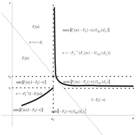
= max{F1(u)−F0(−v), GM L(d0)} u≥u0, v≥v0 oru≥d0−v, v1≤v < v0

= 1−F0(−v) u≥d0−v, v < v1

The regions are as in Figure 1. Using this figure it is easily checked that the c.d.f. has the correct marginal distributionsF0(y) and 1−F1(−y).

The joint distribution of Y1,−Y0 is singular, because all probability is

con-centrated on two curves

S1={(u, v)|v=−F

−1

0 (1−F1(u)), u≤u0}

and

S2={(u, v)|v=−F

−1

0 (F1(u)−GM L(d0)), u > u0}

If GM L(d0) > 0 (we only consider this case; if GM L(d0) = 0 the analysis is

slightly different), the curveS1 is increasing in uand is equal to v1 if u=u0.

The curve S2 is ∞ if u = u0 and converges to v1 as u → ∞. Moreover if

˜

uminimizesF1(u)−F0(−(d0−u)) (the minimand need not be unique), then

F1(˜u)−F0(−(d0−u˜)) =GM L(d0)) so that

d0−u˜=−F

−1

0 (F1(˜u)−GM L(d0))

and we conclude thatS2 touches the line u+v =d0 at all minimands ˜u. The

same argument shows that S2 cannot be below the line u+v = d0. The two

curves are drawn in Figure 1 for the case that there is a unique minimand ˜u. The c.d.f. Gd0L(d) that supports the lower Makarov bound ind0is obtained

by computing the probability mass in the set{(u, v)|u+v≤d}. Ford≤d0

Gd0L(d) = GM L(d0) u0+v1≤d≤d0

= F1(u(d)) d < u0+v1 (2)

withu(d) the solution to

Fig 1. Definition and support ofGd0L if there is a unique minimand.

i.e. S1 intersects u+v = dat u= u(d), v =d−u(d). Note that Gd0L(d) is

constant ifu0+v1 ≤d≤d0, because the line u+v=u0+v1 intersects S1 at

u=u0, v=v1 and

Gd0L(u0+v1) =Hed0L(u0, v1) =F1(u0) =GM L(d0)

Ford > d0

Gd0L(d) =F1(u2(d))−F0(−(d−u1(d))) (4)

whereu1(d)≤u2(d) are the two solutions to

u=d+F−1

0 (F1(u)−GM L(d0))

i.e. the two points of intersection ofS2andd−u.

Note that ford0, d1Gd0L(d) =Gd1L(d) for alld∈ ℜiffGM L(d0) =GM L(d1).

Therefore

Theorem 4.1 The lower Makarov bound GM L is uniformly sharp on a set

whereGM L is constant. The same holds for the upper Makarov bound. On sets

Although according to Theorem 2.2 pointwise sharp bounds are c.d.f. they need not have all the properties ofG. We show this in an example which we will use as an illustration throughout this paper.

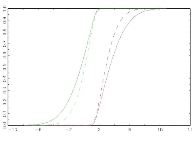
Example 1: Difference of normals with the same variance. Consider

Yk∼N(µk, σ2) k= 0,1

Define the ATE byθ=µ1−µ0. The lower bound on the c.d.f. of the treatment

effect is

GM L(d) = 0 ifd < θ

= 2Φ

d−θ

2σ

−1 ifd≥θ

The corresponding density is

gM L(d) = 0 ifd < θ

= 1

σφ

_d

−θ

2σ

ifd≥θ

Note that this is the density of a halfnormal distribution with begin point θ. Hence the mean of the lower bound distribution is

θ+σ2

√

2

√

π > θ

and the mean of the lower bound distribution is strictly larger that the mean of the distribution ofY1−Y0. The upper bound is

GM U(d) = 2Φ

d−θ

2σ

ifd < θ

= 1 ifd≥θ

The corresponding density is

gM U(d) =

1

σφ

_d

−θ

2σ

ifd < θ

= 0 ifd≥θ

which is the density of a halfnormal distribution distribution with end pointθ, so that the mean of the upper bound distribution is equal to

θ−σ2

√

2

√

π < θ.

Fig 2. Makarov bounds on the treatment effect c.d.f.: Normal outcome distri-butions with equal varianceθ= 1, σ= 3.

It is also illustrative to give the supporting c.d.f. that passes through the lower boundGM L(d0). For d≤d0 from (3)8

u(d) = d+µ0+µ1 2

Also

u0=µ1+σΦ

−1_(G

M L(d0)) v0=d0−u0 v1=−µ0−σΦ

−1₍₁

−GM L(d0))

8

Therefore

Gd0L(d) = Φ

_d

−θ

2σ

d < u0+v1

= 2Φ

d0−θ

2σ

−1 u0+v1≤d≤d0

= Φ

u2(d)−µ1

σ

−Φ

−(d−u1(d))−µ0

σ

d > d0

withu1(d)< u2(d) the solutions to

u=d+µ0+σΦ

−1

Φ

u−µ1

σ

−GM L(d0)

✷.

The conclusion is that although all c.d.f. in the set of treatment effect distributions have meanθ, the c.d.f. that correspond to the lower and upper Makarov bounds have a mean that is strictly larger and smaller thanθ. Hence they do not have all the properties of the set of c.d.f. that they bound. The Makarov bounds are envelopes of the c.d.f. that support them, i.e. the c.d.f. in (2) and (4). These envelopes need not have a mean equal toθ.

5

Averaging over covariates

The conditional onXMakarov bounds on the conditional treatment effect distri-bution in a pointdare pointwise sharp. If we average these conditional pointwise sharp bounds overX we obtain pointwise sharp bounds on the unconditional treatment effect distribution. To see this we construct the supporting joint c.d.f. conditional onX as in the previous section where we substitute condi-tional outcome distributions for uncondicondi-tional ones. Averaging this supporting conditional joint c.d.f. overX we obtain the unconditional joint c.d.f. that has marginal distributions equal to the given (unconditional) outcome distributions ofY0 andY1. The distribution ofY1−Y0 derived from this average supporting

c.d.f. has a c.d.f. that is equal to the lower or upper average Makarov bounds ind, depending on which supporting c.d.f. we use.

The pointwise sharp average Makarov bounds improve on the bounds derived from the average, i.e. unconditional, outcome distributions.

Theorem 5.1 Averaging over covariates gives tighter bounds, that is,

sup

t

max{E_[F1(t|X)]−E_{[F0(t−d|X)]−,0} ≤}E

sup

t

max{F1(t|X)−F0(t−d|X)−,0}

(5)

Eh_inf

t min{F1(t|X)−F0(t−d|X)−+ 1,1}

i

≤inf

t min{

Proof:See Appendix B.

The theorem shows that the average Makarov bounds are more informative than the Makarov bounds on the average distribution. This means that even in a randomized experiment covariate information can be useful in narrowing the bounds on the c.d.f.. The next example illustrates the role of averaging for normal outcome distributions.

Example 2: Conditional normal outcome distributions. The conditional outcome distributions are

Yk|X ∼N(αk+βkX, σ2) k= 0,1

i.e. they are obtained from linear regression models with normal errors with the same variance that does not depend onX. The ATE given X is θ(X) =

α1−α0+ (β1−β0)X. The conditional lower Makarov bound is

GM L(d|X) = 0 ifd < θ(X)

= 2Φ _d

−θ(X) 2σ

−1 if d≥θ(X)

and the conditional upper Makarov bound is

GM U(d|X) = 2Φ

d−θ(X) 2σ

ifd < θ(X)

= 1 ifd > θ(X)

Hence the average lower bound is

E_{[GM L(d|X)] =}E

I(d≥θ(X))

2Φ _d

−θ(X) 2σ

−1

and the average upper bound is

E_[GM U(d|X)] =E

2I(d≤θ(X))Φ

d−θ(X) 2σ

+I(d > θ(X))

IfX is itself normally distributed then the unconditional outcome distributions are normal

Yk∼N(αk+βkµX, βk2σ2X+σ2)

The Makarov bounds for normal outcome distributions with different variances have an explicit expression that is given in Appendix A. In Figure 3 we plot the average bounds (dashed line) and the bounds for the average (solid line) population forα0= 0, α1= 1, β0= 1, β1= 1.5, σ= 1. The mean and standard

deviation of the normal distribution ofX 1 and .8, respectively. The implied

R2_{in the two outcome distributions are .39 (control) and .59 (treatment). Note}

Fig 3.Average Makarov bounds and Makarov bounds for the average population: conditional Normal outcome distributions with Normally distributed covariate.

6

Bounds on the distribution function of

treat-ment effects in two points

6.1

A necessary condition for being compatible with a

treatment effect c.d.f. in two points

Because the Makarov bounds are pointwise, but not uniformly sharp, the region that these bounds imply for the vector of values of the treatment effect c.d.f. in a vector of points is not necessarily best possible. Let d1 < . . . < dK be K ordered real numbers. We are interested in obtaining bounds on the set of

K-vectors B(d1, . . . , dK) = {((G(d1)· · ·G(dK))′, G ∈ G} with as before G the

G(d2) are within the Makarov bounds we have that

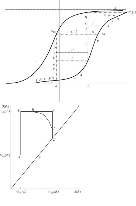
B(d1, d2)⊆ M(d1, d2) =

{(G(d1), G(d2))|GM L(d1)≤G(d1)≤GM U(d1), GM L(d2)≤G(d2)≤GM U(d2), G(d1)≤G(d2)}

The set M(d1, d2) is drawn in the bottom panel of Figure 5. It is the

region bounded by the extreme pointsA, B, C, D, E. For obvious reasons we call

M(d1, d2) the two-dimensional Makarov bounds onG(d1), G(d2). The analysis

is somewhat different for the case that d1 < d2 are ‘close’ in the sense that

GM U(d1)≥GM L(d2). Ifd1, d2 are not close in this sense, the two-dimensional

Makarov bounds are a rectangle, because the monotonicity restriction is not binding. Because we are interested in functionals of the treatment effect c.d.f. that can be approximated by the value of that functional in a finite (but possibly large) number of points on the support of the treatment effect c.d.f. the case thatGM U(dk)≥GM L(dk+1) is the most relevant case.

The two-dimensional Makarov bounds M on the treatment effect c.d.f. in

d1 < d2 contain B. The two-dimensional Makarov bounds are sharp if and

only if M=B. Therefore they are not best possible, if we can find points in

M that are not in B. To establish that a point, e.g. point C in Figure 5 is in B, we would have to construct a joint c.d.f. of Y0, Y1 with given marginal

distributions, such that the c.d.f. of Y1−Y0, i.e. the supporting c.d.f. GC,

satisfiesGC(d1) =GM U(d1) andGC(d2) =GM U(d2). A simpler procedure is

to find necessary conditions for the existence of a supporting c.d.f. GC. If these

conditions do not hold in C, then C /∈ B. The same is true for all points in

Mwhere the necessary conditions do not hold. Therefore, the setB is strictly smaller thanMand by eliminating all points where the necessary condition does not hold, we obtain the maximal reduction relative to the necessary condition. We have been unable to show that our necessary condition for membership of

B is also sufficient. So strictly speaking we cannot call our improved bounds sharp.

To derive the necessary condition forC ∈ B, we note that ifGC ∈ G, then GM L(d) ≤ GC(d) ≤ GM U(d) for all d and the corresponding treatment

ef-fect distribution has meanE_(Y1)−E_{(Y0). In addition, ifGC exists it is larger}

than the smallest c.d.f. GM L ≤ GCK ≤ GM U and smaller than the largest

c.d.f. GM L ≤ GCG ≤ GM U with GCK(d1) = GCG(d1) = GM U(d1) and

GCK(d2) = GCG(d2) = GM U(d2). A c.d.f. F is smaller than a c.d.f. G if

Gfirst-order stochastically dominatesF. Of course, this implies that the mean of the distribution ofGcannot be smaller than the mean of the distribution of

F. Combining these observations we conclude that ifGC exists, then the mean

of GCK is not greater than E(Y1)−E(Y0) and the mean of GCG not smaller

thanE_(Y1)−E_{(Y0). If this necessary condition does not hold then C /∈ B. We}

show how to check the necessary condition and find the smallest set inMwhere this condition is satisfied.

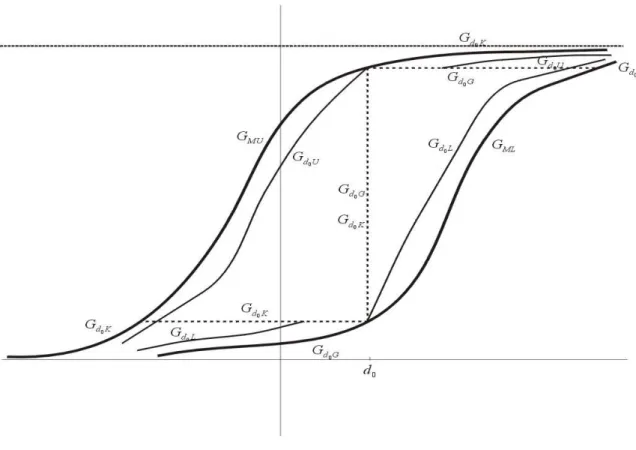
As a first step in the derivation of the necessary condition we derive the stochastically smallest distributionGd0Kthat is within the Makarov bounds and

is within the Makarov bounds and passes throughGM U(d0). The construction

is illustrated in Figure 4.

Gd0K(d) = GM U(d) d < G

−1

M U(GM L(d0))

= GM L(d0) G−M U1 (GM L(d0))≤d < d0 (7)

= GM U(d) d≥d0

Gd0G(d) = GM L(d) d < d0

= GM U(d0) d0≤d < G

−1

M L(GM U(d0)) (8)

= GM L(d) d≥G

−1

M L(GM U(d0))

Note thatGd0K(d0) =GM U(d0)> GM L(d0) =Gd0K(d0)−. However, Gd0K is

Fig 4. The smallest c.d.f. Gd0K through the lower Makarov bound, the largest c.d.f. Gd0G through the upper Makarov bound and the c.d.f. Gd0L, Gd0U that support the bounds.

smaller than all c.d.f. that have Gd0K′(d0) = GM L(d0) and calling Gd0K the

BecauseGd0K is the smallest c.d.f. within the Makarov bounds that passes

throughGM L(d0), it is first-order stochastically dominated by the c.d.f. Gd0L

that supports the lower boundGM L(d0). Because this distribution has a mean

equal toE_(Y1)−E_{(Y0) we conclude that the mean of the distribution of Gd}

0K

cannot be larger thanE_(Y1)−E_{(Y0). In the same way the mean of the}

distri-bution ofGd0G cannot be smaller thanE(Y1)−E(Y0). Therefore the necessary

condition is met for the Makarov bounds in a single point, because the largest c.d.f. corresponding to GM L(d0) and the smallest corresponding to GM U(d0)

are the Makarov boundsGM LandGM U. Note thatGd0K andGd0G are mixed

discrete-continuous distributions with a support that is the union of two disjoint sets and an atom ind0.

Stochastically smallest and largest c.d.f. that are within the Makarov bounds and pass through a particular point can also be constructed in the two-dimensional case.

Lemma 6.1 Let d1< d2 be such that GM U(d1)≥GM L(d2). The mean of the smallest c.d.f. that passes through B,C,D, and E and is within the Makarov bounds is smaller than or equal toE_(Y1)−E_{(Y0). The mean of the largest c.d.f.}

that passes through A,B,D and E and is within the Makarov bounds is larger than or equal toE_(Y1)−E_(Y0).

Proof:See Appendix B.

Consider a point inB(d1, d2) which is equal toG(d1), G(d2) for someG∈ G.

The c.d.f. Gfirst-order stochastically dominates the smallest c.d.f. that passes throughG(d1) and G(d2) and is within the Makarov bounds, Gd1d2K, and it

is first-order stochastically dominated by the largest c.d.f. that passes through

G(d1) andG(d2) and is within the Makarov bounds,Gd1d2G. Hence a necessary

condition for (G(d1), G(d2)) ∈ B(d1, d2) is that Gd1d2K has a mean that does

not exceed the ATE andGd1d2G has a mean that is not smaller than the ATE.

Theorem 6.1 If (G(d1), G(d2)) ∈ B(d1, d2) for some G ∈ G, then the mean of the distribution with c.d.f. Gd1d2K is less than or equal to E(Y1)−E(Y0) and the mean of the distribution with c.d.f. Gd1d2G is greater than or equal to

E_(Y1)−E_(Y0).

Lemma 6.1 implies that B,D, and E are in B(d1, d2). However, it is not

obvious that A and C are in this set. To decide this we construct the smallest c.d.f. that passes through A (see Figure 5). We only need to consider the smallest c.d.f. because the largest c.d.f. that passes through A is equal to the lower Makarov bound and has a mean that is larger than or equal to the ATE. Ifd1< d2are close so thatGM U(d1)≥GM L(d2), the smallest c.d.f. that passes

through A is

GAK(d) = GM U(d) d < G

−1

M U(GM L(d1))

= GM L(d1) G

−1

M U(GM L(d1))≤d < d1

= GM L(d2) d1≤d < d2 (9)

We show that this c.d.f. can have a mean that is larger than the ATE and in that caseA /∈ B(d1, d2). For C the smallest c.d.f. that passes through this point

and is within the Makarov bounds is the c.d.f. of the upper Makarov bound with a mean that is smaller than or equal to the ATE. The largest c.d.f. within the Makarov bounds that passes through C is (ifd1 < d2 are close as defined

above)

GCG(d) = GM L(d) d < d1

= GM U(d1) d1≤d < d2

= GM U(d2) d2≤d < G

−1

M L(GM U(d2)) (10)

= GM L(d) d≥G

−1

M L(GM U(d2))

and this c.d.f. may have a mean that is less than or equal to the ATE, and in that caseC /∈ B(d1, d2).

We compute the mean of the distribution in (9) by subdividing the sup-port in the interval (−∞, G−1

M U(GM L(d1))), the pointd1, the pointd2 and the

interval [d2,∞). The distribution corresponding to the c.d.f. assigns positive

probability to these points and intervals and zero probability elsewhere. By partial integration we find

µAK =

Z G−1

M U(GM L(d1))

−∞

sdGM U(s) +

Z ∞

d2

sdGM U(s) + (11)

d1[GM L(d2)−GM L(d1)] +d2[GM U(d2)−GM L(d2)] =

GM L(d1)G

−1

M U(GM L(d1))−

Z G−1

M U(GM L(d1))

−∞

GM U(s)ds+

Z ∞

d2

(1−GM U(s))ds

+d1[GM L(d2)−GM L(d1)] +d2[1−GM L(d2)]

An analogous argument gives the mean ofGCG

µCG =

Z d1

−∞

sdGM L(s) +

Z ∞

G−1

M L(GM U(d2))

sdgM L(s) + (12)

d1[GM U(d1)−GM L(d1)] +d2[GM U(d2)−GM U(d1)] =

G−1

M L(GM U(d2))(1−GM U(d2)) +

Z ∞

G−1

M L(GM U(d2))

(1−GM L(s))ds−

Z d1

−∞

GM L(s)ds

+d1GM U(d1) +d2[GM U(d2)−GM U(d1)]

Because the density gM U is the density of a halfnormal distribution with

endpointθ, we can use the truncated normal mean formula9 _{to derive}

Z b

−∞

sdGM U(s) =

2θΦ b−θ

2σ

−4σφ b−θ

2σ

ifb < θ

θ−4σφ(0) ifb≥θ

and Z θ

a

sdGM U(s) = 2θ

₁

2 −Φ _a −θ 2σ +4σ φ _a −θ 2σ

−φ(0)

ifa < θ

In this example GM U(d1) ≥ GM L(d2) iff d2 ≥ d1 ≥ θ or d1 ≤ d2 ≤ θ or

d1< θ < d2 and

d1

σ −2Φ

−1

Φ

_d

2−θ

2σ −1 2 ≥ θ σ

This restriction is assumed to hold in the rest of the example.

Upon substitution of the integrals above in (11) we obtain the mean of the smallest distribution that passes through A. If d1 < d2 ≤ θ, then

be-cause GM L(d1) = GM L(d2) = 0, so that in the truncated mean formula b =

G−1

M U(GM L(d1)) =−∞anda=d2

µAK= 2θ

₁

2 −Φ _d

2−θ

2σ

+ 4σ

φ

_d

2−θ

2σ

−φ(0)

+ 2d2Φ

_d

2−θ

2σ

.

Thus, becaused2−θ≤0, we have thatµAK≤θsince

µAK−θ= 4σ

φ

d2−θ

2σ

−φ(0) +

d2−θ

2σ

·Φ

d2−θ

2σ

≤0.

Therefore ifd1≤d2< θ, then A∈ B(d1, d2).

If θ ≤ d1 < d2, we have GM U(d2) = 1, b = G

−1

M U(GM L(d1)) = θ +

2σΦ−1 _Φ d1−θ

2σ

−1 2

≤θanda=d2> θ. Thus

µAK = 2θ

Φ

d1−θ

2σ

−1₂

−4σφ

Φ−1

Φ

d1−θ

2σ

−1₂

+2d1

Φ

_d

2−θ

2σ

−Φ _d

1−θ

2σ

+ 2d2

1−Φ

_d

2−θ

2σ

If for example,θ= 1, σ= 3 andd1= 1.5, d2= 2.5, thenµAK = 1.3814>1 =θ

so thatA /∈ B(d1, d2).

9

IfY has a normal distribution with meanµand varianceσ2

, then

E(Y|a≤Y ≤b) =µ+σ

φa−_σµ−φb−_σµ

Finally, ifd1< θ < d2 then becauseGM L(d1) = 0, GM U(d2) = 1 and in the

truncated mean formula b=G−1

M U(GM L(d1)) =−∞and a=d2 > θ (so that

the truncated means are 0)

µAK = d1

2Φ

d2−θ

2σ

−1

+ 2d2

1−Φ

d2−θ

2σ

If, for example,θ= 1, σ = 3 and d1 =−1 andd2 = 2, thenµAK = 1.60290 >

1 =θso thatA /∈ B(d1, d2).

The densitygM Lis the density of halfnormal distribution with support [θ,∞)

and again using the truncated normal mean formula Z ∞

a

sdgM L(s) =

θ+ 4σφ(0) ifa≤θ

2θ 1−Φ a−θ

2σ

+ 4σφ a−θ

2σ

ifa > θ

and Z b

θ

sdgM L(s) = 2θ

Φ

b−θ

2σ

−1₂

+ 4σ

φ(0)−φ

b−θ

2σ

If we substitute these expressions in (10) we obtain an expression forµCG. We

distinguish between the cases thatd1< d2≤θ, thatθ < d1≤d2, and thatd1<

θ < d2. We maintain the restrictions that ensure thatGM U(d1)≥GM L(d2).

Ifθ < d1≤d2, we haveGM U(d2) = 1,GM U(d1) = 1,a=G−M L1 (GM U(d2)) =

∞,b=d1, so that

µCG= 2θ

Φ

d1−θ

2σ

−1₂

+4σ

φ(0)−φ

d1−θ

2σ

+2d1

1−Φ

d1−θ

2σ

and therefore

µCG−θ

2σ = 2

φ(0)−φ

d1−θ

2σ

+2

d1−θ

2σ

−2

d1−θ

2σ

Φ

d1−θ

2σ

≥0

Hence ifθ < d1< d2, thenC∈ B(d1, d2).

If d1 < d2 ≤ θ, we have GM L(d1) = 0 and in the truncated means a =

G−1

M L(GM U(d2)) =θ+ 2σΦ−1 Φ d2₂−σθ

+1₂,b=d1< θ, so that

µCG = 2θ

₁

2 −Φ _d

2−θ

2σ

+ 4σφ

Φ−1

Φ

_d

2−θ

2σ

+1

2

+2d2

Φ

_d

2−θ

2σ

−Φ _d

1−θ

2σ

+ 2d1Φ

_d

1−θ

2σ

If for example,θ= 1, σ= 3 andd1=−0.5, d2= 0.5, thenµCG= 0.6186<1 =θ

andC /∈ B(d1, d2).

Finally, ifd1< θ < d2thenGM L(d1) = 0,GM U(d2) = 1,a=G

−1

M L(GM U(d2)) =

∞, andb=d1< θ, so that

µCG = 2d1Φ

d1−θ

2σ

+d2

1−2Φ

d1−θ

2σ

If, for example,θ= 1, σ= 3 andd1=−1,d2= 2, thenµCG=−0.2166<1 =θ

6.2

More informative bounds on the treatment effect c.d.f.

in two points

The example shows that µAK can be larger and µCG can be smaller than the

ATE so that either A or C (or both) are not in B(d1, d2). By continuity, if

e.g. A /∈ B(d1, d2), then the points in a neighborhood ofAare also not in that

set. We will determine the (largest) subset ofM(d1, d2) that is not inB(d1, d2).

That subset is drawn in Figure 5, i.e. the region bounded by A,F and G. If

C /∈ B(d1, d2), then the largest subset of M(d1, d2) that is not in B(d1, d2) is

bounded byI,H, andC in Figure 6.

Theorem 6.2 If the smallest c.d.f. GM L≤GAK ≤GM U that passes through GM L(d1) and GM L(d2) has a mean µAK > E(Y1)−E(Y0) then all points in

M(d1, d2)below the convex curveG2=P(G1) defined by

E_(Y1)−E_{(Y0) =}

Z G−1

M U(G1)

−∞

sgM U(s)ds+d1[min{G2, GM U(d1)} −G1] (13)

+ Z G−1

M U(G2)

d1

sgM U(s)ds+d2[GM U(d2)−G2] +

Z ∞

d2

sgM U(s)ds

= G−1

M U(G1)G1−

Z G−1

M U(G1)

−∞

GM U(s)ds

+1(G2 > GM U(d1))

"

G−1

M U(G2)−d1GM U(d1)−

Z G−1

M U(G2)

d1

GM U(s)ds

#

+d1[min{G2, GM U(d1)} −G1] +d2[1−G2] +

Z ∞

d2

(1−GM U(s))ds

(where we adopt the convention that an integral is 0 if the upper integration limit is smaller than the lower integration limit and1(.)is the indicator function) are not inB(d1, d2).

If the largest c.d.f. GM L≤GCG≤GM U that passes through GM U(d1) and

GM U(d2) has a meanµCG<E(Y1)−E(Y0)then all points inM(d1, d2)above the concave curveH2=Q(H1)defined by

E_(Y1)−E_{(Y0) =}

Z d1

−∞

sgM L(s)ds+d1[H1−GM L(d1)] +

Z d2

G−1

M L(H1)

sgM L(s)ds+

(14)

d2[H2−max{H1, GM L(d2)}] +

Z ∞

G−1

M L(H2)

sgM L(s)ds=

−

Z d1

−∞

GM L(s)ds+d1H1+1(GM L(d2)> H1)

"

d2GM L(d2)−G

−1

M L(H1)H1−

Z d2

G−1

M L(H1)

GM L(s)ds

# +

d2[H2−max{H1, GM L(d2)}] +G

−1

M L(H2)(1−H2) +

Z ∞

G−1

M L(H2)

are not in B(d1, d2). The set C(d1, d2) bounded by M(d1, d2) and the curves (13) and (14) is convex.

Proof:See Appendix B.

IfG2≤GM U(d1) the curveP has an explicit expression

P(G1) =

−(E_(Y1)−E_{(Y0)) +d2+}R∞

d2(1−GM U(s))ds−d1G1+G

−1

M U(G1)G1−

RG−1

M U(G1)

−∞ GM U(s)ds

d2−d1

and the same is true forQifH1≥GM L(d2)

Q(H1) =

−(E_(Y1)−E_{(Y0)) +d2H2−}R∞ G−1

M L(H2)(1−GM L(s))ds+G

−1

M L(H2)(1−H2)−

Rd1

−∞GM L(s)ds

d2−d1

Theorem 6.2 defines a subsetC(d1, d2) ofM(d1, d2) that contains B(d1, d2).

If the mean of the smallest c.d.f. that passes through A is larger than the ATE and/or the largest c.d.f. that passes through C is smaller than the ATE, thenC(d1, d2) is a strict subset ofM(d1, d2) and we have bounds that are more

informative than the two-dimensional Makarov bounds.

It follows directly from the construction that GF K˜ (d1)≤GH G˜ (d2) so that

in Figures 5 and 6 G is below I. This implies that the projection ofC_{(d1, d2)}

are the original Makarov bounds in d1 and d2, respectively. In other words,

althoughC_{(d1, d2) may be smaller thanM(d1, d2), the projections are equal to}

the Makarov bounds in a single point.

All results until now hold also for the conditional (onX) bounds. We now show that the specific shape of the improved bounds implies that averaging over X makes them more informative. By Theorem 6.2 C(d1, d2) is bounded

by the one-dimensional Makarov bounds (vertical and horizontal bounds) , the curves (13) and (14), and the 45 degree line. If the bounds are obtained from conditional outcome distributions, then it follows from Theorem 5.1 that the horizontal and vertical lower bounds cannot decrease if we average, that the horizontal and vertical upper bounds cannot increase if we average. Finally, by Jensen’s inequality the convex curve (13) cannot decrease and the concave curve (14) cannot increase if we average. Together with the observation that the 45 degree line is unaffected by averaging, we have

Theorem 6.3 Let C(d1, d2)(X) be the convex set defined in Theorem 6.2 as derived from the conditional outcome distributions, thenE_[C_{(d1, d2)(X)]cannot}

be larger thanC(d1, d2)that is derived from the unconditional outcome distribu-tions.

Example 1, continued: Difference of normals with the same variance. We found that for θ = 1, σ = 3 and d1 = 1.5, d2 = 2.5 A /∈ B(d1, d2). For

these valuesµCG= 1.4834>1 so thatC∈ B(d1, d2). Therefore we only have a

For d1 = −0.5, d2 = 0.5, we found that C /∈ B(d1, d2). However, µAK = .5166 so thatA∈ B(d1, d2) and we only have a more informative upper bound

that is drawn in Figure 8.

Finally, for d1 =−1 and d2 = 2, A /∈ B(d1, d2) and C /∈ B(d1, d2). Both

the lower and upper Makarov bound can be improved and the more informative bounds are in Figure 9. ✷

7

Bounds on functions of the distribution of

treat-ment effects

The boundsC(d1, d2) on the c.d.f. of the treatment effect distribution ind1and

d2 imply bounds on functions of the treatment effect c.d.f. ind1< d2. Here we

consider linear functions ofG(d1), G(d2)

B(G(d1), G(d2)) =b1G(d1) +b2G(d2)

Ifb1= 1, b2=−1 this function is equal to the interval probabilityG(d2)−G(d1).

Another parameter that can be approximated byBis the total net gain for those individuals whose net gain is between 0 andC.

Z C

0

(1−G(s))ds

If we divide the integration region in two intervals [0, c) and [c, C], then an approximation is

C−cG(c/2)−(C−c)G((c+C)/2)

If we pickd1=c/2, d2= (c+C)/2, b1=c, b2=C−c we obtain bounds on the

total gain from bounds onB. In the sequel we can, without loss of generality, assume thatb2>0.

Manski (1997b), (2003) introduces the concept of a D parameter which is some increasing functional of a c.d.f. where the c.d.f. are ordered according to first-order stochastic dominance. The linear functional that we consider is a D parameter iffb1, b2≥0. An interval probability, and in general the linear

functional withb1≥0 andb2<0, is not a D parameter, but it can be expressed

a difference of D parameters. Manski derives bounds for D parameters and differences of D parameters. These bounds are different from ours, because he assumes that outcomes are weakly increasing in the level of treatment. We do not make his assumption, in particular we do not assume that everybody benefits from the treatment.

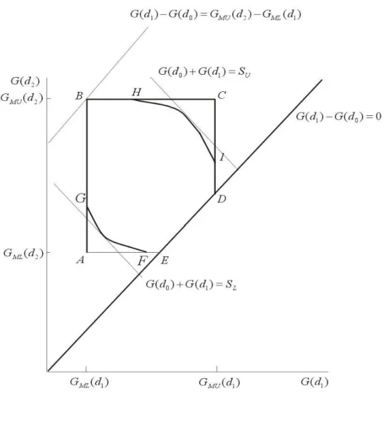
In Figure 10 we draw the set C(d1, d2). In the sequel we use the notation

G1 ≡G(d1) and G2 ≡ G(d2). The bounds on B(G1, G2) depend on whether

µAK Rθ andµCGRθ. B(G1, G2) is minimal in D, E or A ifµAK ≤θand in

D, E, a point at whichB touches P(G1), F or G ifµAK > θ. The latter is a

µAK > θ, then the point at whichB(G1, G2) is minimal is determined by the

slope of B(G1, G2) and the slope of P(G1) in F and G. The upper bound of

B(G1, G2) is determined in a similar way. Therefore we define

P′

F ≡P

′

(P−1_(G

M L(d2)))

P′

G≡P

′

(GM L(d1))

Q′

H≡Q

′

(GM U(d1))

Q′

I ≡Q

′

(Q−1_(G

M U(d2)))

The bounds onB(G1, G2) that we denote byBL≤BU are given in the following

theorem.

Theorem 7.1 If µAK≤θ, then the lower bound onB(G1, G2) is

BL = b1GM U(d1) +b2GM U(d1) if b1<−b2

= b1GM L(d2) +b2GM L(d2) if −b2≤b1<0

= b1GM L(d1) +b2GM L(d2) if b1>0

IfµAK > θ, then the lower bound on B(G1, G2)is

BL = b1GM U(d1) +b2GM U(d1) if b1<−b2

= b1GM L(d2) +b2GM L(d2) if −b2≤b1<0

= b1P

−1_(G

M L(d2)) +b2GM L(d2) if 0< b1≤ −b2P

′

F

= b1G˜1+b2P( ˜G1) if −b2PF′ < b1<−b2PG′

= b1GM L(d1) +b2P(GM L(d1)) if b1≥ −b2P

′

G

whereG˜1 is the unique solution to

P′

( ˜G1) =−

b1

b2

If µCG≥θ then the upper bound is

BU = b1GM L(d1) +b2GM U(d2) if b1<0

= b1GM U(d1) +b2GM U(d2) if b1>0

and ifµCG< θ

BU = b1GM L(d1) +b2GM U(d2) if b1<0

= b1Q−1(GM U(d2)) +b2GM U(d2) if 0< b1<−b2Q′H

= b1H˜1+b2Q( ˜H1) if −b2Q

′

H< b1≤ −b2Q

′

I

= b1GM U(d1) +b2Q(GM U(d1)) if b1≥ −b2Q′I

whereH˜1 is the unique solution to

Q′

( ˜H1) =−

b1

Example 1, continued: Difference of normals with the same variance. We consider bounds on the functions

B1(G1, G2) =G2−G1

and

B2(G1, G2) =G1+G2

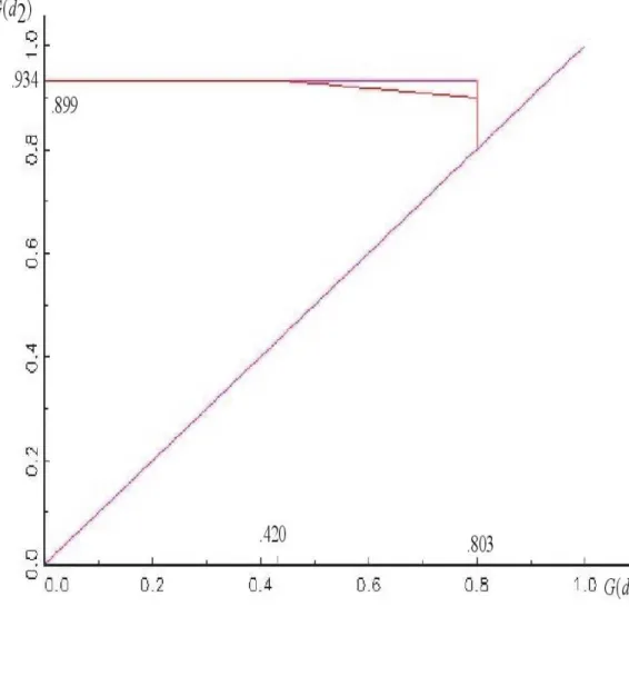
Ifθ= 1, σ= 3 and d1= 1.5, d2= 2.5 the bound in Figure 7 implies that

0≤B1(G1, G2)≤.934

with no improvement over the Makarov bounds. ForB2(G1, G2)

.298≤B2(G1, G2)≤2

and this improves on the Makarov bounds that are

.263≤B2(G1, G2)≤2

Ford1=−0.5, d2= 0.5 we obtain from the bound that is drawn in Figure 8

0≤B1(G1, G2)≤.934

with no improvement and

0≤B2(G1, G2)≤1.703

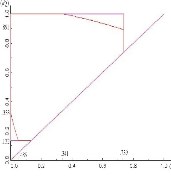
where the upper bound improves on the Makarov bound that is 1.737. Finally, ford1=−1 andd2= 2 the bound are in Figure 9 gives

0≤B1(G1, G2)≤1

which is noninformative and

.617≤B2(G1, G2)≤1.630

which improves considerably on the Makarov bounds

.132≤B2(G1, G2)≤1.739

✷

8

Conclusion

sharp with the latter implying the former, but the former not implying the latter. Uniformly sharp bounds are members of the set that is being bounded. Pointwise sharp bounds share some of the properties of the set, but not all. This fact implies thatKdimensional bounds on the value of the function inK

points may not be best possible. We consider bounds on the set of treatment effect c.d.f. with given marginal outcome distributions. The Makarov bounds on this set are pointwise sharp but in general10 not uniformly sharp, because their mean is in general not equal to the Average Treatment Effect. We have shown that this allows us to narrow the higher dimensional Makarov bounds. Because the set bounded by the improved bounds is convex, it is straightforward to use these bounds obtain bounds on linear functionals. In some cases the improved higher dimensional bounds narrow the bounds on the functionals substantially. We give explicit expressions for the bounds on the set and on linear functionals for K = 2. These expressions can be generalized to arbitrary K. Moreover, because the set is convex, averaging over covariates that are correlated with the outcomes will narrow the bounds even further.

REFERENCES

Aakvik, A., J. Heckman, and E. Vytlacil, (2005) “Estimating Treat-ment Effects for Discrete Outcomes when Responses to TreatTreat-ment Vary: an ap-plication to Norwegian vocational rehabilitation programs,”Journal of Econo-metrics, 125, 15-51.

Abadie, A., (2002), “Bootstrap Tests for Distributional Treatment Effects in Instrumental Variable Models,”Journal of the American Statistical Associa-tion, 97, 284-292.

Abadie, A., (2003), “Semiparametric Instrumental Variable Estimation of Treatment Response Models,”Journal of Econometrics, 113, 231-263.

Abadie, A., J. Angrist, and G. Imbens, (2002), “Instrumental Vari-ables Estimates of the Effect of Subsidized Training on the Quantiles of Trainee Earnings,”Econometrica, 70, 91-117.

Carneiro, P., K. Hansen, and J. Heckman, (2003), “Estimating Distri-butions of Treatment Effects with an Application to the Returns to Schooling and Measurement of the Effects of Uncertainty on College Choice,” Interna-tional Economic Review, 44, 361-422.

10

Djebbari, H, and J. Smith, (2008), “Heterogeneous Impacts in PRO-GRESA, ”Journal of Econometrics, 145, 64-80.

Easterlin, R., (2008), “Lost in Transition: Life Satisfaction on the Road to Capitalism, ” Working Paper, No. 3409, IZA, Bonn

Fan, Y., S. Park, (2007), “Sharp Bounds on the Distribution of the Treat-ment Effect and Their Statistical Inference, ” typescript, DepartTreat-ment of Eco-nomics,Vanderbilt University.

Firpo, S., (2007), “Efficient Semiparametric Estimation of Quantile Treat-ment Effects,”Econometrica, 75, 259-276.

Frank M., R. Nelsen, and B. Schweizer, (1987), “Best-Possible Bounds for the Distribution of a Sum–a Problem of Kolmogorov,” Probability Theory and Related Fields, 74, 199–211.

Fr´echet, M., (1951), “Sur les Tableaux de Corr´elation dont les Marges Sont Donn´ees,”Annals University Lyon, Series A, 53-77.

Heckman, J., and J. Smith, (1993), “Assesing the Case for Randomized Evaluation of Social Programs,” in Jensen, K and P. Madsen (Eds.) Measuring Labour Measures: Evaluating the Effects of Active Labour Market Policy Initia-tives, Copenhagen, Ministry Labour.

Heckman, J., and J. Smith, (1998), “Evaluating the Welfare State,” in S. Strom (Ed.) Econometrics and Economic Theory in the 20th Century: The Ragnar Frisch Centennial, Econometric Soceity Monograph Series, Cambridge, Cambridge University Press.

Heckman, J., J. Smith, and N. Clements, (1997), “Making the Most out of Programme Evaluations and Social Experiments Accounting for Hetero-geneity in Programme Impacts,”Review of Economic Studies, 64, 487-535.

Hoeffding, W., (1940), “Masstabinvariate Korrelations-Theorie,” Scri-ftenreite Math. Inst. Univ. Berlin, 5, 181–233.

Imbens, G., and D. Rubin, (1997), “Estimating Outcome Distributions for Compliers in Instrumental Variables Models,”Review of Economic Studies, 64, 555–574.

Makarov, G., (1981), “Estimates for the Distribution Function of a Sum of Two Random Variables when the Marginal Distributions are Fixed,”Theory of Probability and its Applications, 26, 803-806.

Manski, C., (1997a), “The Mixing Problem in Programme Evaluation,”

Review of Economic Studies, 64, 537–553.

Manski, C., (1997b), “Monotone Treatment Response,”Econometrica, 65, 1311-1334.

Manski, C., (2003), Partial Identification of Probability Distributions (Springer Series in Statistics), Springer-Verlag, New York.

Rabin, M.,(1998), “Psychology and Economics,”Journal of Economic Lit-erature 36, 11-46.

Tversky, A., and D. Kahneman, (1991), “Loss Aversion in Riskless Choice: A Reference-Dependent Model,”Quarterly Journal of Economics 106, pp.1039-61.

A

Makarov bounds on the treatment effect

dis-tribution if the marginal outcome

distribu-tions are normal with unequal variances

IfYk ∼N(µk, σ2k), k= 0,1, then withθ=µ1−µ0

GM L(d) = Φ



−σ1(d−θ) +σ0 q

(d−θ)2_{+ 2(σ}2

0−σ21) ln

σ0

σ1

σ2 0−σ12

 ₋

Φ 

−σ0(d−θ) +σ1 q

(d−θ)2_{+ 2(σ}2

0−σ21) ln

σ0

σ1

σ2 0−σ12

 

GM U(d) = Φ



−σ1(d−θ)−σ0 q

(d−θ)2_{+ 2(σ}2

0−σ21) ln

σ0

σ1

σ2 0−σ12

 ₋

Φ 

−σ0(d−θ)−σ1 q

(d−θ)2_{+ 2(σ}2

0−σ21) ln

σ0

σ1

σ2 0−σ12

 + 1

B

Proofs

Proof of Theorem 3.1:

First consider the lower bound. We have for allv, uwithv+u=dand using the Bonferroni inequality

G(d|x) = Pr(Y1+ (−Y0)≤d|X =x)≥Pr(Y1≤u,−Y0≤v|X =x)≥

max{Pr(Y1≤u|X=x)+Pr(−Y0≤v|X =x)−1,0}= max{F1(u|x)−F0(−v|x)−,0}

Hence if we definet≡u, d≡u+v

G(d)≥E

sup

t

max{F1(t|X)−F0(t−d|X)−,0}

For the upper bound we have

1−G(d|x) = Pr(Y1+ (−Y0)> d|X =x)≥Pr(Y1> u,−Y0> v|X =x)≥

max{Pr(Y1> u|X =x) + Pr(−Y0> v|X =x)−1,0}

Taking the opposite on both sides of the equation, adding 1, substituting t ≡

u, d≡u+v, and taking the expectation gives

G(d)≤Eh_inf

t min{F1(t|X)−F0(t−d|X)−+ 1,1}

We show that the bounds are themselves c.d.f. Consider the lower bound for

G(d|x)

GM L(d|x) = sup

t max{F1(t|x)−F0(t−d|x)

−,0}

Now ifd′

≥d, then for allt

max{F1(t|x)−F0(t−d

′

|x)−,0} ≥max{F1(t|x)−F0(t−d|x)−,0}

so thatGM L(d′|x)≥GM L(d|x). Next we show thatGM L(d|x) is right

continu-ous. Consider a sequencedn↓d. First the sequenceGM L(dn|x) is nonincreasing

and bounded from below, so that it has a limit. Obviously 0≤dn−d < εiff

0 ≤(t−d)−(t−dn) < ε independent of t. Hence for all δ > 0 and n large

enough

F0(t−dn|x)≥F0(t−d|x)−−δ

because t−dn ↑ t−d andF0(.)− is the left-hand limit. Using this inequality we have for allt

F1(t|x)−F0(t−d|x)− ≤F₁(t|x)−F₀(t−dn|x)− ≤F₁(t|x)−F₀((t−d)|x)−+δ

Taking the sup overtfrom right to left we obtain

GM L(d|x)≤GM L(dn|x)≤GM L(d|x) +δ

Taking the limit we obtain, becauseδis arbitrary, that limn→∞GM L(dn|x) = GM L(d|x), so that the lower bound is right-continuous. Note that

GM L(d|x)≥F1(d/2|x)−F0(−d/2|x)

so that limd→∞GM L(d|x) = 1. Taking the expectation over X we conclude

that the lower bound is indeed a c.d.f. (by dominated convergence limits and expectations can be interchanged). The proof that the upper bound is also a c.d.f. is analogous.

Proof of Theorem 3.2:

LetGL be decreasing ind0, so that for somed′ < d0 GL(d′)> GL(d0). The

supporting c.d.f. Gd0L is such thatGd0L(d0) =GL(d0). ThereforeGd0L(d

′ )< GL(d′) which implies thatGd0L∈ G/ . In the same way we show that the lower

bound is 0 and 1 at −∞ and ∞, respectively. If GL is discontinuous at d0

and not right-continuous, thenGL(d0)< GL(d0)+. The supporting c.d.f. Gd0L

satisfies Gd0L(d0) = GL(d0) and because Gd0L ∈ G also Gd0L(d) ≥ GL(d0)+

for d > d0. Therefore the supporting c.d.f. is not right-continuous in d0, a

contradiction. We prove in the same way thatGU is a c.d.f. ✷

Proof of Theorem 5.1:

For allx∈ X and alls∈ ℜ

sup

t