APPLICATION OF PREDICTIVE CONTROL TECHNIQUES WITHIN
PARALLEL ROBOT
Fabian Andres Lara-Molina
∗João Maurício Rosário
∗Didier Dumur
†Philippe Wenger
‡∗UNICAMP - Mechanical Engineering School, Campinas - SP, Brazil
†SUPELEC Systems Sciences (E3S) - Automatic Control Department, Gif sur Yvette, France
‡IRCCyN - Institut de Recherche en Communications et Cybernétique de Nantes, Nantes, France
ABSTRACT
Aplicação de Técnicas de Controle Preditivo em Robô Paralelo
Este trabalho apresenta a aplicação de técnicas de cont-role preditivo para rastreamento de trajetórias de um robô paralelo. A estratégia de controle preditivo generalizado (GPC), que considera o modelo dinâmico linearizado, é us-ada para melhorar a precisão de rastreamento das trajetórias. O controlador preditivo generalizado é robustificado devido ao ruído de medição e dinâmicas não modeladas utilizando parametrização Youla. É realizada Uma simulação do robô Orthoglide considerando as incertezas dos parâmetros ge-ométricos e dinâmicos, ruído nos sensores e atritos para duas trajetórias diferentes. Finalmente, o controlador GPC robus-tificado e a técnica de Controle de Torque Computado (CTC) são comparadas. Os resultados das simulações mostram que o controlador GPC robustificado apresenta um melhor de-sempenho para altas acelerações e também reduz o efeito do ruído no sinal de controle do robô paralelo.
KEYWORDS: Robô Paralelo, Controle Robótico, Controle
Preditivo Generalizado
Artigo submetido em 24/03/2011 (Id.: 1307) Revisado em 28/05/2011, 26/09/2011, 29/11/2011
Aceito sob recomendação do Editor Associado Prof. Luis Fernando Alves Pereira
ABSTRACT
This paper addresses the position tracking control applica-tion of a parallel robot using predictive control techniques. A Generalized Predictive Control strategy (GPC), which con-siders the linear dynamic model, is used to enhance the track-ing position accuracy. The robustification of GPC against measurement noise and neglected dynamics using Youla pa-rameterization is performed. A simulation of the orthoglide robot considering uncertainties related to geometrical and dynamic parameters, sensors noise and frictions is performed on two different trajectories. Finally, it is compared the ro-bustified GPC controller with the classical Computed Torque Control (CTC). The robustified GPC controller shows a bet-ter performance for high accelerations and it also reduces the effect of the noise in the control signal of the parallel robot.
KEYWORDS: Parallel robot, Robot control, Generalized
pre-dictive control
1
INTRODUCTION
Generally, the actuators are nearby or mounted on the fixed basis deliver the mechanical power to the mechanism.
Due to their mechanical structure, they have some conceptual advantages over serial robots, such as, higher stiffness, accu-racy, payload-weight ratio and better dynamic performance. However, they have more kinematic and dynamic complexi-ties than serial robots.
According to their characteristics, the parallel robots have been used widely in industrial applications such as ”pick and place“ robots (Briot and Bonev, 2010), machine tools (Weck and Staimer, 2002) and precision surgery robots (Wapler et al., 2003) among others.
Although theoretically parallel robots have some potential advantages, it is still difficult to take advantage of them (Abdellatif and Heimann, 2010). To reach a high perfor-mance in industrial applications, their dynamical potential advantages should be exploited completely. Consequently, it is essential to reduce the execution time and to increase the accuracy in order to improve the productivity and quality of manipulation and production processes that use parallel robots (Pietsch et al., 2005).
Two factors affect the accuracy of parallel robots. First, passive joints produce kinematic model errors due to clear-ances and assembly defects (Wang and Masory, 1993). Sec-ond, singularities within workspace volume produce a de-creasing of the stiffness resulting in a lack of accuracy for a given task, this problem has been addressed through path planning (Dasgupta and Mruthyunjaya, 1998). Therefore, parallel robots still need improvements in design, model-ing and control in order to reach their theoretical capabilities (Merlet, 2002). As seen, many works address modeling and design; nevertheless, there are few works related to parallel robot control.
Mainly two control approaches have been considered for par-allel robots in literature: dynamic control, which is based on dynamic model of these robots (Paccot et al., 2009), (Wanga et al., 2009); and adaptive control which adjusts the parame-ters of the system or controller online (Pietsch et al., 2005). Additionally, dynamic control techniques as CTC does not deal very well with modeling errors. They create a pertur-bation on the error behaviors which may lead to a lack of stability and accuracy (Dombre and Khalil, 2010).
In the other hand, model based predictive control techniques have been applied to parallel robots; Belda et al. (Belda et al., 2003) designed a generalized predictive control law (GPC) for path control of redundant parallel robots; Poignet et al. (Vivas and Poignet, 2005) applied functional predictive control based on the simplified dynamic model of H4 paral-lel robot; Duchaine et al. (Duchaine et al., 2007) presented a
predictive control law for position tracking and velocity con-trol considering the dynamic of the robot. Nevertheless, it is necessary to have robust control laws towards model uncer-tainties such as measurement noise and parameter uncertain-ties; in this way, an acceptable behavior of control actions is ensured with an improvement of the dynamic performance of parallel robots.
In this paper, we use GPC to enhance the dynamic perfor-mance of a parallel robot in the position tracking control. Then we compare the GPC performance with the classical robot controller: Computed Torque Control (CTC). First, the dynamic equation of the robot is linearized in order to apply the linear control laws. After that, based on the linear model, we apply GPC and CTC control in each actuator of the paral-lel robot. We robustify the GPC controller toward model un-certainties via Youla parameterization. Finally, we perform the simulation considering uncertainties related to geometric and dynamic parameters, sensors noise and frictions of the complete model of the Orthoglide parallel robot; thus, the performance of CTC and robustified GPC controllers is eval-uated in terms of tracking accuracy and control actions char-acteristics using two different workspace trajectories. We evaluate the behavior of tracking accuracy and disturbance rejection in order to compare the controllers performance.
This paper is organized in five sections. In section 2, CTC controller is presented. Section 3 sumarizes GPC design pro-cedure and the robustification of GPC. Section 4 presents the kinematic and dynamic model of the Orthoglide paral-lel robot. In section 5, simulations are performed and results are presented. Finally, we present the conclusion and further work.
2
CONTROL OF PARALLEL KINEMATICS
MACHINES IN RST FORM
In this section, we present the Computed Torque Control (CTC) of the parallel robots in the joint space. Finally, we introduce the representation of the CTC in the RST form.
CTC is composed of two independent loops: an inner-loop to linearize the non-linear dynamic of the robot and an outer loop to track a desired trajectory. Thus, the non-linear dy-namic equation of the robot is considered as follows:
Γ=A(q)¨q+h(q,q˙) (1)
whereq,q˙ andq¨are the joint space position, velocities and
The robot equations may be linearized and decoupled by non-linear feedback. Aˆ(q)andhˆ(q,q˙)are respectively the
estimates of A(q) and h(q,q˙). Assuming that Aˆ(q) =
A(q)andhˆ(q,q˙) = h(q,q˙), the problem is reduced to a nlinear and decoupled double-integrators system, wheren
is the number of degrees of freedom of the robot (Khalil and Dombre, 1999).
¨
q=w (2)
Withwbeing the new input control vector, the equation (2) corresponds to the inverse dynamic control scheme, where the dynamic of the robot is transformed into a double set of integrators (see Fig. 1). Thus, linear control techniques can then be used to design a tracking position controllers, such as the model-based predictive control (CARIMA model of section 3).
Let us assume that the desired trajectory for each actuator is specified with the desired positionqd, velocityq˙dand
accel-erationq¨d. The outer-loop of the controller is:
w= ¨qd+KP(qd−q)+KD
d
dt(q
d−q)+K
I Z t
0
(qd−q)dτ
(3) whereKP =diag(k, . . . , k),KD =diag(kTD, . . . , kTD),
KI=diag(k/TI, . . . , k/TI).
+ ☛ ✡ ✟ ✠ ☛ ✡ ✟ ✠ ☛ ✡ ✟ ✠ ... ... ... . ...... ............ ... . ✲ ✲ ✲ ............ ... . ✲ ✲ ❄ ✲ ... ... ... ... ✣ ✲ ............ ... . ✲ ✲ ✻ ❄ ✛ ✛ ✻ ✻ Non-linear compensation + qd
K
IR
dτ
K
P ˙ qdK
V ¨ qd +ˆ
A
(
q
)
w + Γ
+
Robot
ˆ
h
(
q
,
q
˙
)
˙ q q +− + − + ☛ ✡ ✟ ✠
Figure 1: CTC controller, block diagram.
The controller gains are found in order to have in continuous-time domain the following closed-loop characteristic equa-tion for each decoupled double-integrator (sis the Laplace variable)
(s+ωr)(s2+ 2ξωrs+ωr2) = 0 (4)
Thus,k= (1 + 2ξ)ω2
r,kTD= (1 + 2ξ)ωrandk/TI =ω3r.
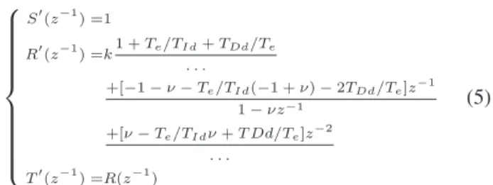
The two degrees of freedom RST digital controller is a stan-dard control form in industry (Landau, 1998). CTC con-troller is expressed in RST form using the Euler transform with sample periodTeand a low pass filter withN TD time
constant for the derivative action, being N a constant. Thus,
S′ (z−1
) =1
R′ (z−1
) =k1 +Te/TId+TDd/Te . . .
+[−1−ν−Te/TId(−1 +ν)−2TDd/Te]z −1
1−νz−1
+[ν−Te/TIdν+T Dd/Te]z−2 . . .
T′ (z−1
) =R(z−1
)
(5)
where, z−1 is the backward shift operator, T
Id = 2TI,
TDd = 1+N TN Te/2Te D andν = 1+N T1−N Tee/2T/2TDD. Fig. 2 shows the
CTC controller in RST form.
Plant
☛ ✡ ✟ ✠ ☛ ✡ ✟ ✠ ✲ ❄ ✲ ... ... ... . ...... ............ ... . ✲ ✲ ✻ ✲ ...... ... . ...... ✲ ✲ ✻T
′(z
−1)
R
′(z
−1)
+
− 1 ∆S′(z−1) qd ¨ qd
Robot
q Γ + +ˆ
A
(
q
)
ˆ
H
(
q
,
q
˙
)
+ + w ☛ ✡ ✟ ✠Figure 2: CTC controller in RST form.
3
PREDICTIVE CONTROL TECHNIQUES
This section has two parts. In the first part, the GPC proce-dure design is presented. In the second part is presented the GPC controller robustification using Youla parameterization.
3.1
GPC Design
This section presents the principles and briefly describes the formulation of GPC law to introduce the design procedure and implementation on the parallel robot. This control tech-nique was developed by Clarke et al. (Clarke et al., 1987). Predictive control philosophy can be summarized as follows: 1) definition of a numerical model of the system to predict the future behavior, 2) minimization of a quadratic cost func-tion over a finite future horizon, using future predicted errors, 3) elaboration of a sequence of future control values, apply-ing only the first value both on the system and the model, 4) iteration of the whole procedure at the next sampling period according to the receding horizon strategy.
us-ing the Euler transform andTesample period to findA(z−1)
andB(z−1)polynomials of the model.
A(z−1)y(t) =B(z−1)u(t−1) + ξ(t)
∆(z−1) (6)
With u(t), y(t) the plant input and output andξ(t) a cen-tered Gaussian white noise. The control signal is obtained by minimization of the quadratic cost function:
J=
N2
X
j=N1
[r(t+j)−yˆ(t+j)]2+λ
Nu
X
j=1
∆u(t+j−1)2 (7)
WhereN1andN2define the output prediction horizons, and
Nudefines the control horizon.λis a control weighting
fac-tor,rthe reference value,yˆthe prediction output value,
ob-tained solving diophantine equation, anduthe control
sig-nal. The receding horizon principle assumes that only the first value of optimal control series resulting from the opti-mization ofδJ/δu is applied, so that for the next step this procedure is repeated. Thus, the design has been performed adjustingN1,N2,Nu,λto satisfy the required input/output
behavour: fastest response consistent with stability require-ments; with this control strategy a 2-DOF RST controller is obtained, the procedure is described in (Boucher and Du-mur, 1995).
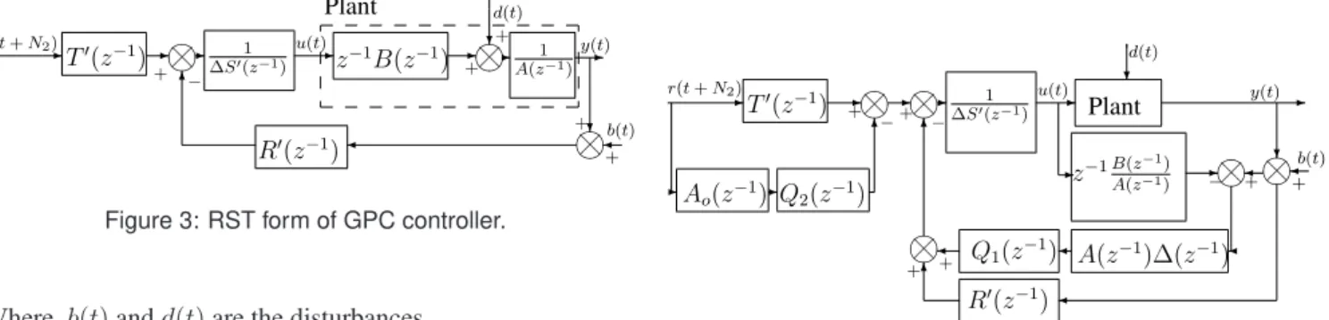
S′(z−1)∆(z−1)u(t) =−R′(z−1)y(t) +T′(z)r(t) (8)
The resulting RST controller is showed in Fig. 3.
Plant ☛ ✡ ✟ ✠ ☛ ✡ ✟ ✠ ............ ... .. ... ... ... . ...... ... ... ... . ...... ✻ ✛ ✛ ❄ ✲ ✲ ✲ ❄ ✲ ✲ ✲ ✲
z−1B(z−1)
T′(z−1) 1
A(z−1)
R′(z−1) 1 ∆S′(z−1)
+ + + − + + d(t)
y(t)
b(t) u(t)
r(t+N2)
☛ ✡
✟ ✠
Figure 3: RST form of GPC controller.
Where,b(t)andd(t)are the disturbances.
3.2
GPC Robustification
GPC may significantly improve performances in terms of accuracy. Nevertheless, disturbances due to measurement noise or neglected dynamics within the model might affect the robot performance and hence control actions. In this way the robustification of the controllers against these uncertain-ties is important.
Initially, the procedure starts with GPC design, in our case in RST form. Then, the robustness of the GPC controller is
enhanced via Youla parameterization with regards to model uncertainties, while respecting time domain constraints, such as disturbance rejection. This parameterization allows for-mulating frequency and time-domain constraints as convex optimization. This optimization problem is approximated by a linear programing with inequality constraints, and the opti-mal parameters belonging to the research space set.
The set of all stabilising controllers of the system, shown in Fig. 4, which are given follows the Youla parametrization (Kouvaritakis et al., 1992) as follows:
T(z−1) =T′(z−1)−A
o(z−1)Q2(z−1)
R(z−1) =R′(z−1) + ∆(z−1)A(z−1)Q
1(z−1)
S(z−1) =S′(z−1)−z−1B(z−1)Q1(z−1)
(9)
where Q1(z−1)andQ2(z−1)are stable transfer functions,
andAoAc= ∆AS′+z−1BR′the characteristic polynomial
of the closed loop of Fig. 3, this characteristic polynomial is split into a control polynomialAc and an observer
polyno-mialAo.
Since Q2(z−1) modifies the input/output, to remain this
transfer function unchanged, Q2(z−1) = 0. On the other
hand, onlyQ1(z−1)is considered, since this parameter does
not modify the input/output transfer function. This parame-terization allows formulating frequency constraints (robust-ness to model uncertainties) and time domain constraints (disturbance rejection) as convex optimization.
1 ∆S′(z−1
) ☛ ✡ ✟ ✠ ☛ ✡ ✟ ✠ ☛ ✡ ✟ ✠ ☛ ✡ ✟ ✠ ✲ ✻ ✛ ✛ ✛ ...... ... ... ... . ✛ ✲ ❄ ✲ ✲ ✻ ✲ ...... ... . ...... ✲ ✲ ✲ ✲ ❄ ✲ ✛ ✛ ✻ ...... ... ... ... . ............ ... . ... ... ... .. ...... + + −
R′(z−1)
+
Q1(z−1)
Ao(z−1) Q2(z−1)
A(z−1)∆(z−1)
z−1B(z−1
) A(z−1)
Plant
−
+
T′(z−1)
r(t+N2) u(t)
b(t) y(t) d(t)
+ − + ☛ ✡ ✟ ✠
Figure 4: Robustified RST structure.
In this way, we consider the uncertainty block∆u(z−1)
con-nected to the system in Fig. 5(a). ∆u(z−1) represents an
unstructured multiplicative direct uncertainty (M’Saad and Chabassier, 1996). The uncertainty block is connected to the
P(z−1) =E(z−1)/V(z−1)system as shown in Fig. 5(b).
whereP(z−1)is the transfer function seen by the uncertainty
r(t+N2) ☛
✡ ✟
✠ ✲
✲
... ... ... . ...... ...
... ... . ......
✻
✛ ❄ ✲ ✲ ✲
✲ ✲
v(t) e(t)
P(z−1)
+ ∆u(z−1)
z−1 B(z−1
) A(z−1)
1 ∆S(z−1)
+
−
+
y(t) u(t)
R(z−1)
T(z−1) ☛
✡ ✟ ✠
(a) Unstructured multiplicative direct uncertainty.
v(t)
✛
✲P(z−1) ∆u(z−1)
e(t)
(b)P(z−1
)system connected to uncertainty block.
Figure 5: System connected to uncertainty.
P(z−1) =−z−1BR′
AoAc
−z−
1B∆A
AoAc
Q1 (10)
The parameterQ1(z−1)results from optimization problem.
It takes into account frequencies for which the model has more uncertainties and measurement noise influence than al-lowed by theΦenv1(Q1)in equation (11). Also, time
time-domain specification, such as disturbance rejection dynam-ics, in terms of the transfer disturbance/output is denoted by
Φenv2(Q1)in equation (11). The robustness is maximized
where anH∞norm is minimized in the following way
min
Q1∈ℜH∞
Φenv1(Q1)<0
Φenv2(Q1)<0
P(z−1)W(z−1)
∞ (11)
where W(z−1)is a weighting transfer function which
de-notes the frequency ranges where model uncertainties are more important.
The disturbances d(t) and b(t) affect the signals u(t) and
y(t). In equation (12), the transfer functions are linearly parametrized by Youla parameter Q1 (Kouvaritakis et al.,
1992). These transfer functions must be considered for the time-domain constraint problem.
u y
=
Hud Hub
Hyd Hyb
d b
(12)
Assuming thats(t)ij is the response of Hij transfer
func-tion to a specific input, the time-domain constraint deliver the limits in whichs(t)ij must be restricted. TheQ1parameters
that satisfied this constraint are expressed in the following way
Cenv={Q1/∀t≥0;smin(t)≤s(t)ij ≤smax(t)} (13)
={Q1/Φenv(Q1)≤0}
with:
Φenv(Q1) = max
max
t≥0(s(t)ij−s(t)max, smin(t)−s(t)ij)
(14) Full developments of the method are given in (Rodriguez and Dumur, 2005).
4
TEST-BED MODEL
4.1
Description
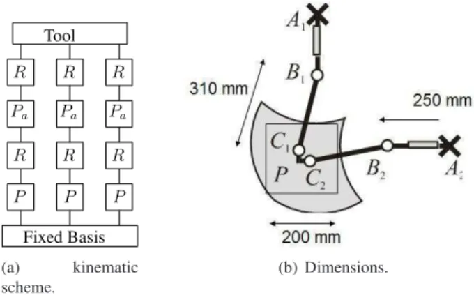
Orthoglide is a parallel robot with three translational degrees of freedom (Fig. 6). The Orthoglide mechanical structure has a movable platform, three prismatic actuators, and three iden-tical kinematic chains P RPaR (P prismatic, R rotational,
Pa parallelogram, see Fig. 6(a)). The actuated joints are
the three orthogonal prismatic ones at the fixed basis. The workspace volume is free of singularities and self collisions (see Fig. 6(b)), thus Orthoglide is useful for many tool paths.
P R
Pa
R
P
Fixed Basis Tool
R
Pa
R
P R
Pa
R
(a) kinematic
scheme.
(b) Dimensions.
Figure 6: Orthoglide Robot, description.
Orthoglide robot was designed for high-speed machining, thus the machine reaches a tool velocity of 1.2m/sand an acceleration of 20m/s2at the isotropic configuration,
4.2
Geometric and kinematic modeling
In the model, the active joints are q =
q11 q12 q13
T
associated to the linear actuators. The passive joints are
q21 q22 q23 q31 q32 q33
T
. The Inverse Geometric Model (IGM) delivers the actuator positionsqas function of Cartesian position of end effector 0p
P = xp yp zp T
, such as Fig. 7 presents, thus:
q11
q12
q13
=
zpcos(q31) cos(q21)d41−d61
xp−xA2−cos(q32) cos(q22)d42−d62
yp−yA3−cos(q33) cos(q32)d43−d63
(15)
where:
q31= sin−1(−d41yp);q21=−(sin
−1( −xp cos(q31)d41) +
π 2)
q32= sin−1(−zp+zA
2
d42 );q22=−(sin
−1(−yp+yA2
cos(q32)d42) +
π 2)
q33= sin−1(−xp+xA
3
d43 );q32=−(sin
−1( −zp+zA3
cos(q33)d43) +
π 2)
The direct geometric model is reduced to a simple equation of second order such as is presented at (Pashkevich et al., 2006):
xp
yp
zp
=
qb1/2−t1/qb1
qb2/2−t1/qb2
qb3/2−t1/qb3
(16)
where:
qbi=qbi+d4i, fori= 1,2,3.
t1 = −B−
√
B2
−4AC
2A , A = q 2
11q122 + q112 q213 + q212q132 ,
B = q2
11 + q122 + q132 and C = (q112 +q122 +q132 −
4d2
41)/(q211q122 q132 )/4
The Inverse Kinematic Model (IKM) delivers actuators ve-locitiesq˙ =
˙
q11 q˙12 q˙13
T
as function of Cartesian ve-locity of the end effector0v
P =x˙p y˙p z˙p T
:
˙
q= 0J−P10vP (17)
where,0J−1
P is the inverse Jacobian matrix of the robot, thus:
0J−1
P =
− 1
tan(q21)
tan(q31)
sin(q21) 1
1 − 1
tan(q22)
tan(q32)
sin(q22)
tan(q33)
sin(q23) 1 −
1 tan(q23)
(18)
The second order inverse kinematic model gives the actua-tors accelerationsq¨ =
¨
q11 q¨12 q¨13
T
as function of the
Cartesian platform acceleration0v˙
P, and actuator velocities
˙ q:
¨
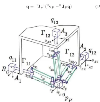
q= 0J−1
P (0v˙P −0J˙Pq˙) (19)
Figure 7: Orthoglide Robot, Geometric CAD.
4.3
Dynamic modeling
The Cartesian accelerations of the end effector 0v˙ P can be calculated using the direct dynamic equation of the Or-thoglide. It is written in the following form (Guegan et al., 2007):
0v˙
P =A(q)−robot1 [0J− T
P Γ−h(q,q˙)robot] (20)
where:
• A(q)robot =P3i=1[A(q)ix] +I3mpis the total inertia
matrix (3x3) of the robot, the inertia of kinematic chains and movable platform.
• Γ=
Γ11 Γ12 Γ13
T
is the actuators force vector.
• h(q,q˙)robot = P3i=1[hix(qi,q˙i)−A(q)ix0J˙iq˙i]−
mpg
• h(q,q˙)ix is the Coriolis, gravitation, and centrifuge
force vector (3x1). A(q)ix is the inertia matrix (3x3)
of each kinematic chain.
• mp is the mass of the movable platform, g =
Therefore, the numerical integration of the direct dynamic equation allows to simulate the dynamics of the robot. The dynamic parameters of the robot correspond to masses, iner-tias and frictions identified in (Guegan et al., 2003).
5
SIMULATION AND RESULTS
In order to establish a framework to compare the perfor-mance of the controllers, we simulated the dynamic response of the Orthoglide robot and we use the following controllers CTC and GPC, thus the control laws have been tested in sim-ulation in Matlab / SimulinkR.
5.1
Simulation
We simulated the dynamic response of the Orthoglide robot using the following controllers CTC and GPC in order to es-tablish a performance comparison in terms of tracking ac-curacy and disturbance rejection. The controller parameters were set according to the procedure design presented earlier.
The robot behavior is simulated using the direct dynamic model of the parallel robot in equation (20). Uncertainties about dynamic parameters, errors in geometric parameters (due to assembly tolerances), fictions and Gaussian noise on sensors (variance 1. 10−9) are included in the simulation
(Fig. 8).
✲ ✻
✲ ❄
✻
✲ ✲ ✲.............
... ✲
✻
Robot
Dynamic equation
˙
vP PP
q
+
+
50µmError on
Γ
R
R
IGM
IKM vP
0
˙
vP =A(q)−
1
robot[
0
J−T
P Γ−h(q,q˙)robot]
geometrical parameters
q q˙
noiseb(t)
✞ ✝☎✆
Figure 8: Orthoglide robot, simulation of complete model.
In order to provide a CTC/GPC comparison which makes sense, tuning of both controllers were performed as stated below, looking for the same input/output behavior. Further-more, the tuning parameters were also adjusted in order to obtain similar frequency features for the open controlled loop (in terms of phase and gain margins in the bode diagram in particular).
CTC controller is tuned using the following parameters:ξ=1 to guarantee response without overshoot and ωr=50rad/s
obtained experimentally from the parameter identification of the robot; leading tok= 7500,kTD= 150,k/TI = 125000
and a filter of the derivative action withN = 30. CTC
con-troller is implemented in RST in Fig. 2 using the Euler trans-form with sample periodTe=2.5ms. In the same way, GPC
was also tuned to obtain the same input/output behaviour with the same bandwith and damping ratio as for CTC, lead-ing to the followlead-ing set of parameters: N1=1,N2=10,Nu=1
andλ=1.10−9. This was assessed by comparing the Bode
di-agram of the controlled loop. Furthermore robustification of GPC and filtering the derivative effect in the CTC controller leads to the same effect with respect to noise amplification. In that sense, both controllers were tuned in a similar way.
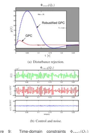
0 0.05 0.1 0.15 0.2 0.25 −5
0 5 10 15 20 25 30 35
Tr = 0.22 →
→
Max = 35
←
Min = −3.5 Φenv1(Q1)
t [s]
y
(
t
)
Robustified GPC
GPC
(a) Disturbance rejection.
0 0.05 0.1 0.15 0.2 0.25 −1
0 1x 10
−4
b
(
t
)
Φenv2(Q1)
0 0.05 0.1 0.15 0.2 0.25 −50
0 50
u
(
t
)
G
P
C
0 0.05 0.1 0.15 0.2 0.25 −50
0 50
u
(
t
)
R
G
P
C
temps(s)
(b) Control and noise.
Figure 9: Time-domain constraints Φenv1(Q1) and
Φenv2(Q1).
To robustify the GPC controller, the optimization problem of equation (11) has to be solved satisfying the two time do-main constraints:Φenv1(Q1)andΦenv2(Q1). The constraint
Φenv1(Q1)corresponds to a time domain template for
dis-turbance rejection y(t)/d(t), the template of this constraint is shown in Fig. 9(a). The constraintΦenv2(Q1)corresponds
to a time domain constraint for measurement noise/control transfer function u(t)/b(t), this specification restricts the noise effect on control signal, therefore the variation ofu(t)
is limited to a range of+/−1 for this application. Fig 9(b) shows the fixed limits in control signal and the measurement noise. Finally, the selected weighting function is
W(z−1) = 1−0.6z−
1
Another aspect for the comparison of the controllers is the computational complexity. The computational cost of the implementation of inverse dynamic model for the inner loop to linearize the robot dynamics is addressed in (Guegan et al., 2003). The outer loop for CTC and GPC controllers corresponds to the difference equations of each RST polyno-mial. The RST polynomials of CTC controller are presented in equation (5). The RST polynomials of GPC controller are obtained through an off-line optimization, the order of RST polynomials for this application are 3, 2 and 10 respectively. In the same way the GPC controller is robustified using the off-line optimization of equation (11), thus for this case the order of RST polynomials for this application are 8, 7 and 15 respectively. Consequently, the computational complexity is rather similar for both controllers, the advantage of the RST form being only the need for a few additions and multiplica-tions, which goes very fast in real time.
5.2
Tracking position error
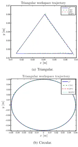
With the purpose of comparing the behavior of CTC and GPC controllers, two workspace trajectoriespdon thex−y
plane are used: 1) a triangular one (edge length = 50mm), with a fifth-degree polynomial interpolation; thus it has a smooth joint space trajectory, at the points where the di-rection of the trajectory changes the initial acceleration is 1m/s2 to test the behavior of the controllers (Fig. 10(a));
and 2) a circular one (∅=50mm, Fig. 10(b)), the initial con-ditions velocity and acceleration are zero.
Fig 10 presents the respective workspace trajectories using CTC, GPC and RGPC. The highest acceleration on the end effector, for these workspace trajectories, is 5m/s2.
Initially, we can see that the workspace trajectories are closer to reference using GPC and RGPC controllers (Fig. 11(b)). GPC and RGPC controllers improve the tracking of the workspace trajectory, since with this controller the robot softly follows the abrupt changes in direction, due to the an-ticipative effect of the predictive control (Fig. 11(a)).
In order to establish the total tracking error of the three actu-ators of robot over a trajectory the Root Mean Square Error (RMSE) of the actuators is evaluated:
RM SE(e) = 1
3m
m
X
k=1
q
e(k)Te(k) (22)
where,e(k)is the error vector of the three actuators for each
kinstant.
In Fig. 12, the maximum acceleration of the end effec-tor varies from 1m/s2 to 5m/s2 for triangular workspace
trajectory (Fig. 12(a)) and circular workspace trajectory
0.01 0.02 0.03 0.04 0.05 0.06 0.07 0.01
0.02 0.03 0.04 0.05 0.06
0.07 Triangular workspace trajectory
x[m]
y
[m
]
pd
CTC GPC RGPC
(a) Triangular.
−0.05 −0.04 −0.03 −0.02 −0.01 0 0.01 0.02 0.03 0.04 0.05 −0.05
−0.04 −0.03 −0.02 −0.01 0 0.01 0.02 0.03 0.04 0.05
Triangular workspace tra jectory
x[m]
y
[m
]
pd
CTC GP C RGP C
(b) Circular.
Figure 10: Workspace trajectories.
(Fig. 12(b)). For both trajectories, when acceleration creases, tracking accuracy decreases because RMSE in-creases. However, using the GPC and RGPC controllers, the increase of RMSE is smaller than using CTC controller; thus, the GPC and RGPC offer a better tracking accuracy. Hence, for parallel robots that operate at high accelerations (high dy-namics), the GPC and RGPC controllers performance is bet-ter than CTC controllers according to the increase of accel-eration.
The Fig. 13 shows measurement noise effect in the control signal on actuators for triangular and circular trajectories. The noise affects more the CTC and GPC control signals than the RGPC control signals. The noise in the control signal us-ing CTC and GPC are very high since the nominal actuators force is 400N.
0.036 0.038 0.04 0.042 0.044 0.046 0.05
0.052 0.054 0.056 0.058 0.06 0.062
Triangular workspace trajectory
x[m]
y
[m
]
pd
CTC GPC RGPC
(a) Triangular.
0.0002 0.0004 0.0006 0.0008 0.001
30
210
60
240 90
270 120
300 150
330
180 0
Tracking Error
[m]
[
m
]
pd CTC GPC RGPC
(b) Circular.
Figure 11: Tracking workspace trajectory and errors.
6
DISTURBANCE REJECTION
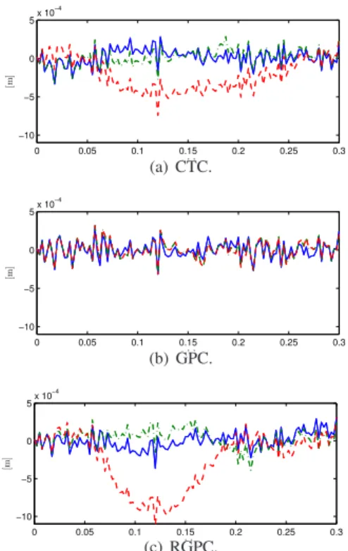
Fig. 14 shows the joint space error when a step load of 1Kg
is applied in the end effector of the robot. Although the re-sults in terms of tracking position accuracy of the GPG are better than the CTC, robustying GPC against noise decreases the dynamics of the closed-loop, thus transient of disturbance rejection is increased as shown Fig. 14(c). This is the main compromise to be fulfilled using the Youla parameter for ro-bustification: trade-off between noise rejection and perfor-mances in terms of disturbance rejection. This trade-off can be adjusted by means of tuning parameters present in equa-tion 11 (mainly envelops definiequa-tion).
7
CONCLUSIONS
The simulation of Orthoglide parallel robot for a position tracking control using GPC, RGPC and CTC controllers is analyzed. In order to apply these control laws, the parallel robot was decoupled and linearized by feedback; after that, CTC and GPC controllers were applied to the linear equiva-lent model.
1 1.5 2 2.5 3 3.5 4 4.5 5 0.1
0.15 0.2 0.25 0.3
0.35RMS Error and Max. aceleration
Max. aceleration [m/s2]
R
M
S
E
[m
m
]
CTC GPC RGPC
(a) Triangular.
1 1.5 2 2.5 3 3.5 4 4.5 5 0.12
0.13 0.14 0.15 0.16 0.17 0.18 0.19 0.2
0.21 RMS Error and Max. aceleration
Max. aceleration [m/s2]
R
M
S
E
[m
m
]
CTC GPC RGPC
(b) Circular.
0 0.05 0.1 0.15 0.2 0.25 0.3 0.35 0.4 0.45 −1000
0 1000
t[s]
Γ
[N]
CTC
0 0.05 0.1 0.15 0.2 0.25 0.3 0.35 0.4 0.45 −1000
0 1000
t[s]
Γ
[N]
GPC
0 0.05 0.1 0.15 0.2 0.25 0.3 0.35 0.4 0.45 −1000
0 1000
t[s]
Γ
[N]
Robustified GPC (a) Triangular.
0 0.1 0.2 0.3 0.4 0.5 0.6 0.7 0.8 0.9 −2000
−1000 0 1000 2000
t[s]
Γ
[N]
CTC
0 0.1 0.2 0.3 0.4 0.5 0.6 0.7 0.8 0.9 −2000
−1000 0 1000 2000
t[s]
Γ
[N]
GPC
0 0.1 0.2 0.3 0.4 0.5 0.6 0.7 0.8 0.9 −2000
−1000 0 1000 2000
t[s]
Γ
[N]
Robustified GPC (b) Circular.
Figure 13: Control signal on actuators.
0 0.05 0.1 0.15 0.2 0.25 0.3 −10
−5 0 5x 10
−4
t[s]
[m
]
(a) CTC.
0 0.05 0.1 0.15 0.2 0.25 0.3 −10
−5 0 5x 10
−4
t[s]
[m
]
(b) GPC.
0 0.05 0.1 0.15 0.2 0.25 0.3 −10
−5 0 5x 10
−4
t[s]
[m
]
(c) RGPC.
Figure 14: Disturbance rejection, error on actuators.
For trajectories typically used in machining, a better per-formance was obtained in terms of tracking accuracy with respect to parameter variation using GPC and RPGC con-trollers; thus, we show that the generalized predictive control improves the dynamic behavior of the parallel robot in terms of tracking error over a trajectory with high acceleration. The robustification of GPC significantly reduces noise in the sig-nal control. In this way the robustification of GPC against these uncertainties is important in the parallel robots.
Further works will develop robust predictive control laws considering the complete model of parallel robots without linearization.
ACKNOWLEDGEMENTS
The authors gratefully acknowledge the support of Fundação de Amparo à Pesquisa do Estado de São Paulo.
REFERENCES
Abdellatif, H. and Heimann, B. (2010). Advanced Model-Based Control of a 6-DOF Hexapod Robot: A Case Study,IEEE/ASME Transactions on Mechatron-ics15(2): 269–279.
generalized predictive control for redundant parallel robots,Mechanics Based Design of Structures and Ma-chines31(3): 413–432.
Boucher, P. and Dumur, D. (1995). Predictive motion control,
Journal of Systems Engineeringpp. 148–162.
Briot, S. and Bonev, I. A. (2010). Pantopteron-4: A new 3T1R decoupled parallel manipulator for pick-and-place applications, Mechanism and Machine Theory
45(5): 707–721.
Clarke, D., Mohtadi, C. and Tuffs, P. (1987). Generalized predictive control. part i. the basic algorithm, Automat-ica23(2): 137–148.
Dasgupta, B. and Mruthyunjaya, T. (1998). Singularity-free path planning for the stewart platform manipulator,
Mechanism and Machine Theory33(6): 711–725.
Dombre, E. and Khalil, W. (2010). Modeling, Performance Analysis and Control of Robot Manipulators, Wiley.
Duchaine, V., Bouchard, S. and Gosselin, C. (2007). Computationally efficient predictive robot control,
IEEE/ASME Transactions on Mechatronics12(5): 570 –578.
Guegan, S., Khalil, W., Chablat, D. and Wenger, P. (2007). Modelisation dynamique d’un robot parallele a 3-DDL : l’Orthoglide, 0707.2185. Conference Internationale
Francophone d’Automatique (07/2002) 1-6.
Guegan, S., Khalil, W. and Lemoine, P. (2003). Identification of the dynamic parameters of the orthoglide,IEEE In-ternational Conference on Conference on robotics and Automation, Vol. 3, pp. 3272–3277.
Khalil, W. and Dombre, E. (1999). Modélisation identifica-tion et commande des robots, Hermes Sciences
Publi-cat.
Kouvaritakis, B., Rossiter, J. A. and Chang, A. O. T. (1992). Stable generalized predictive control: an algorithm with guaranteed stability,Control Theory and Applica-tions, IEE Proceedings D139(4): 349 – 362.
Landau, I. (1998). The R-S-T digital controller design and applications,Control Engineering Practice6(2): 155– 165.
Merlet, J. P. (2002). Still a long way to go on the road for parallel mechanisms,ASME 2002 DETC Conference.
M’Saad, M. and Chabassier, J. (1996).Commande Optimale. Conception Optimisée des systèmes, Paris, France:
Diderot.
Paccot, F., Andreff, N. and Martinet, P. (2009). A review on the dynamic control of parallel kinematic machines: Theory and experiments, The International Journal of Robotics Research28(3): 395–416.
Pashkevich, A., Chablat, D. and Wenger, P. (2006). Kine-matics and workspace analysis of a three-axis parallel manipulator: The orthoglide,Robotica24(1): 39–49.
Pietsch, I., Krefft, M., Becker, O., Bier, C. and Hesselbach, J. (2005). How to Reach the Dynamic Limits of Paral-lel Robots? An Autonomous Control Approach,IEEE Transactions on Automation Science and Engineering
2(4): 369–390.
Rodriguez, P. and Dumur, D. (2005). Generalized predic-tive control robustification under frequency and time-domain constraints, IEEE Transactions on Automatic Control Technology13(4): 577 – 587.
Vivas, A. and Poignet, P. (2005). Predictive functional con-trol of a parallel robot, Control Engineering Practice
13(7): 863–874.
Wang, J. and Masory, O. (1993). On the accuracy of a Stew-art platform. i. The effect of manufacturing tolerances,
IEEE International Conference on Robotics and Au-tomation., Vol. 1, pp. 114–120.
Wanga, J., Wu, J., Wanga, L. and You, Z. (2009). Dynamic feed-forward control of a parallel kinematic machine,
Mechatronics19(3): 313–324.
Wapler, M., Urban, V., Weisener, T., Stallkamp, J., Durr, M. and Hiller, A. (2003). A Stewart platform for precision surgery, Transactions of the Institute of Measurement and Control25(4): 329–334.
Weck, M. and Staimer, D. (2002). Parallel kinematic ma-chine tools – current state and future potentials, CIRP Annals - Manufacturing Technology51(2): 671–683.