Article
J. Braz. Chem. Soc., Vol. 26, No. 10, 1967-1975, 2015. Printed in Brazil - ©2015 Sociedade Brasileira de Química 0103 - 5053 $6.00+0.00
A
*e-mail: [email protected]
Understanding Ozone Concentrations During Weekdays and Weekends in the
Urban Area of the City of Rio de Janeiro
Eduardo M. Martins,a Anna C. L. Nunesa and Sergio M. Corrêa*,b
aFaculdade de Engenharia, Universidade do Estado do Rio de Janeiro, 20559-900 Rio de Janeiro-RJ, Brazil
bFaculdade de Tecnologia, Universidade do Estado do Rio de Janeiro, 20537-000 Resende-RJ, Brazil
In different cities around the world, higher ozone concentrations are observed during weekends for various reasons. This study aims to determine the causes of this effect in the city of Rio de Janeiro based on measurements obtained at three automatic air quality monitoring stations in the Bangu, Campo Grande and Irajá neighborhoods between 2012 and 2013. Variations in the solar radiation and hourly carbon monoxide, nitrogen oxides, non-methane hydrocarbons, ozone and particulate matter concentrations were determined. The Bangu station showed the lowest ozone concentration differences between the weekdays and weekends (8.9%) and recorded the highest ozone concentrations and largest number of exceedances. The low ozone consumption by nitrogen oxide resulted in the high ozone concentrations at the Bangu station. In addition, the
volatile organic compounds (VOC)/nitrogen oxides (NOx) ratio for this station was evaluated for
each day of the week between 6 and 9 AM, and the observed VOC/NOx ratios were higher at the
Campo Grande and Irajá stations. We concluded that the weekend effect occurred at all three of the evaluated stations, with greater intensity at the Campo Grande and Irajá stations. The main cause of this weekend effect is the greater reductions in NO emissions over the weekends, which
increase the VOC/NOx ratio.
Keywords: ozone, weekend, weekday, NOx, VOC, modelling
Introduction
One of the main problems of urban air pollution is the high concentration of photochemical oxidants. Among these oxidants, ozone (O3) is particularly important
because it adversely affects human health, agriculture and materials.1,2
Ozone is a secondary photochemical oxidant that is formed from the reaction of nitrogen oxides (NOx) with
volatile organic compounds (VOCs), which are released into the atmosphere from natural and anthropogenic sources. The formation chemistry of ozone is complex and highly non-linear.3-6 The formation of ozone begins
with the photochemical dissociation of nitrogen dioxide. Tropospheric ozone formation in the absence of VOCs is represented by the reactions in equations 1 through 3.3,4
NO2 + hν→ NO + O(3P) (< 420 nm) (1)
O(3P) + O
2 + M → O3 (2)
O3 + NO → NO2 + O2 (3)
In atmospheres with VOCs, the imbalance between ozone formation and consumption results in the accumulation of ozone in the troposphere. This accumulation results from the two-step oxidation of hydrocarbons. The transformation of NO to NO2 without ozone consumption favors formation processes rather than consumption processes. In the presence of VOCs, the balance between these species is destabilized. The VOCs react through a sequence of reactions with different radicals that are present in the atmosphere, including the OH radical. A sequence of VOC reactions is shown in equations 4-8.
RH + OH → R + H2O (4)
R + O2→ RO2 (5)
RO2 + NO → RO + NO2 (6)
RO + O2→ R’CHO + HO2 (7)
Some of these radicals (HO2 and RO2) react with NO
(equations 5 and 8), converting it to NO2. In addition,
ozone is consumed by the reaction in equation 3. However, as more NO is converted to NO2, the formation of ozone
will increase until the maximum NO2 photolysis rate is
reached.3,4,6
The ozone forming process depends on the VOC/NOx
ratio. At low ratios, the main reaction is between OH and NO2, in which the radical is removed and the formation
of ozone is delayed. Under these conditions, lower NOx
concentrations favor the formation of ozone because more OH radicals become available for reacting with VOCs. In contrast, high VOC/NOx ratios favor reactions with OH
radicals, which increases ozone formation.7
For several years, high ozone concentrations have polluted different cities around the world. In addition, knowledge of ozone forming processes is important for establishing strategies for controlling and reducing ozone concentrations.8 Natural ozone precursor emissions are
not different between weekdays and weekends. However, human activities are significantly different between weekdays and weekends. For example, vehicular traffic, which is a major source of VOC and NOx emissions, is
significantly different between weekdays and weekends.9
The weekend effect of ozone concentrations is easily observed in urban areas and was discovered in the United States in the 70s.5,10 Higher ozone concentrations were
observed during the weekends relative to the weekdays. However, the concentrations of ozone precursors, such as VOCs, NOx and CO, were greater on weekdays. The
changes in the precursor concentrations and ratios were related to changes in the activities and emissions that occurred during the week.
The California Air Resources Board11 identifies
six possible causes for the weekend effect, with the following four main possibilities: (i) the reduction in NOx concentrations, which decreases the VOC ratio
and increases the ozone formation process. Moreover, reductions in the NOx concentration decrease the ozone
formation because the NOx ratio becomes limiting; (ii) the
timing of NOx emissions. Vehicular traffic studies indicated
that vehicle emissions occurred a few hours later during the weekends than during the weekdays; (iii) increased VOCs and NOx in emissions on Friday and Saturday
night could result in greater ozone concentrations after sunrise; (iv) greater sunlight can occur on weekends due to lower particulate matter emissions.5,10-12 Recently, these
possibilities were studied in different countries around the world.7,13-15
The city of Rio de Janeiro covers an area of 1.224 km2
and includes the Serra do Mar mountains in Tijuca,
Gericinó and Pedra Branca, which act as a physical barrier between the waterfront and the mainland. The city has an approximate population of 6.3 million inhabitants with a population density of 5,163.8 inhabitants km−2.16,17 The
city’s fleet of vehicles is estimated at 2,55 million.18
In the city of Rio de Janeiro, the State Environmental Institute (INEA) and the Department of Environment of the City of Rio de Janeiro (SMAC) are responsible for the air quality monitoring network. Automatic monitoring stations are located in urban areas where vehicle emissions are prominent. The following pollutants are monitored at these stations: CO, particulate matter (PM) PM2.5, SO2, NO2,
NO and O3. When considering the pollutant concentrations
throughout the year and comparing them with national and international limits, O3 resulted in the highest number of air
quality standard exceedances. The National Environmental Council-Brazil (CONAMA) resolution 03/90 indicates that the average hourly ozone concentration should not exceed 160 mg m−3. In addition, all stations have recorded
exceedances in the O3 limits in the Municipality of Rio de
Janeiro.19 When assessing and monitored data for 2012
through 2013, the largest number of exceedances occurred at the Bangu, Irajá and Campo Grande stations, with 215, 189 and 77 exceedances, respectively. The highest ozone concentration was observed at the Campo Grande station, with a concentration of 156.9 ppb. Therefore, the data presented in this study demonstrate the necessity of knowing the ozone formation processes in Rio de Janeiro during weekdays and weekends.
Experimental
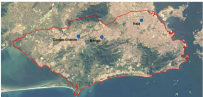
All eight automatic monitoring stations (AMS) of the SMAC are located in an urban area (Figure 1). Thus, most of the pollutant concentrations measured at these stations resulted from vehicle emissions. No significant industrial sources are located near these stations. The three AMSs evaluated in this study are located along Avenida Brasil,
which is the main traffic route, with more than 300.000 vehicles per day according to the inventory of mobile sources.16,17 In Table 1, the monitored pollutants at each
AMS are presented with meteorological parameters, including solar radiation, temperature, humidity, rainfall, wind speed and direction.
To develop this work, Bangu, Campo Grande and Irajá AMSs were chosen, which had the largest number of air quality standard exceedances for ozone. Monitoring primary pollutant concentrations is important for understanding ozone formation processes. The equipment at the stations is frequently calibrated, and data are validated following technical criteria. Ozone was monitored using an Ecotech PTY Serinus 10, NOx was measured using an
Ecotech Serinus 40, nonmethane hydrocarbons (NMHC) were measured using an Ecotech VOC100 model, CO was measured using an Ecotech Serinus 30 and PM10 and PM2.5 were measured using an Ecotech Spirant BAM.
The study period was from January 1, 2012 through December 31, 2013. To assess the existence of the weekend effect on ozone concentrations, the average hourly O3, CO,
NOx, VOCs, PM10 and PM2.5 concentrations and the solar
radiation were monitored. In addition, the average values were calculated for weekdays and weekends.
Weekdays were considered as Monday through Friday, and weekends were considered as Saturdays, Sundays and holidays. Data evaluation was performed using the full data set, with daytime defined as the period between 6 AM to 6 PM and nighttime defined as 7 PM to 5 AM.
The Ox content was used as an indicator of ozone
photochemical production and can be defined by equation 9. Thus, the NO2 concentrations used for
calculating the NOx concentration should represent the
secondary NO2 generated by NO oxidation. Differences in
the Ox concentrations during the weekdays and weekends
were also determined.10,20-22
[Ox] = [O3] + [NO2] – 0.1 × [NOx] (9)
To understand the formation of ozone from VOCs and NOx, a modeling study was performed using the trajectory
model ozone isoplot plotting package (OZIPR) and the chemical mechanism Statewide Air Pollution Research Centre (SAPRC). To support this modeling study and input the VOC reactivity, the different pollutants were speciated. Sixteen air samples were collected using 6 L Entech Silcosteel canisters that were cleaned under high vacuum (bellow 10 mTorr) using an Entech 3100 unit. Samples were collected along the main street of the city during the early morning hours (6-7 AM), corresponding to the rush period, and during low photochemical activity.
Next, VOC speciation was conducted according to the TO-15 U.S.EPAmethodology23 using chromatography
and mass spectrometry (Varian GC450 MS220). The VOC analyses were performed by passing a known volume of sample through a cryogenic pre-concentrator trap (Varian SPT) with TENAX TA and Carbopack B at −60 °C before
injection into a DB-1 60 m column (0.32 mm i.d. with 1.0 µm film). The column temperature was set between 40
and 180 °C, with a heating rate of 6 °C min−1. Quantification
was performed using a five-point calibration curve with the Restek Ozone Precursor Mixture/PAMS 57 components at 100 ppb. The detection and quantification limits were determined using the analytical curve parameters. The detection limit was estimated by multiplying the standard deviation of the linear coefficient from the calibration curve by 3.3 and dividing by its slope. The quantification limit was estimated by multiplying the standard deviation of the linear coefficient from the calibration curve by 10 and dividing by its slope. The limit of detection for all VOC was estimated in 0.75 ppb. After sampling, the canister was connected to a valve positioned in the inlet of the chromatograph. The air inside the canister was removed by using a vacuum pump (Thomas Ind.), and the volume was controlled by mass flow (Sierra Inst. Model 954). After pre-concentrating between 200 and 400 mL of air sample, the VOC was sent to the chromatographic column by fast heating (40 °C s−1) using
Helium 5.0 as the carrier gas.24
Carbonyls samples were collected and analyzed following the U.S.EPA TO-11A methodology.25 The
samples were collected using two SiO2-C18 cartridges
in series, which were impregnated with an acid solution of 2,4-dinitrophenylhydrazine (DNPH) by using an air pump (KNF UNMP 850 KNDC) operated at 1.5 mL min−1
for 60 min. A trap filled with potassium iodide was used before the DNPH cartridge to avoid ozone interference. After sampling, the cartridges were sealed, wrapped with aluminum foil, and stored at 4 °C until analysis. The
Table 1. Monitored pollutants at each automatic monitoring station
AMS CO SO2 O3 PM10 NO2 PM2.5 NMHC
Bangu X X X X X X
Copacabana X X X X
Centro X X X X
Campo Grande X X X X X X
Irajá X X X X X X X
Tijuca X X X X
São Cristóvão X X X X
Guaratiba X X
detailed procedure is thoroughly explained in our previous work.26
The extraction of carbonyl samples was performed using 5 mL of acetonitrile, and chemical analyses were performed using high-performance liquid chromatography (HPLC; Perkin Elmer Series 200 with UV detection at 365 nm). The mobile phase consisted of 55% acetonitrile in water at 30 °C, with a 30 mL volume C18 column (250 mm, 4.6 mm and 5.0 mm). Calibration was performed using a standard mixture (Supelco CARB Carbonyl Mix 1) containing formaldehyde, acetaldehyde, acrolein, acetone, propionaldehyde, butyraldehyde and benzaldehyde at concentrations between 0.1 and 4.0 mg L−1, which yielded
correlation coefficients greater than 0.99.
The modeling procedure was performed using the trajectory model OZIPR, which is widely accepted and well documented in the literature.27,28 Other publications
by our group detail its applicability.29-31
The chemical model used was the 1999 version of the SAPRC model developed by Carter, with several updates added in later years.32-37 This model was widely tested
against 550 controlled experiments in Teflon chambers. The initial version used in this study has 214 reactions with 83 chemical species. Furthermore, our group recently introduced 23 other chemical species and their reactions, which represent species that frequently occur in the Brazilian urban atmospheres, such as ethanol, some alkenes and aromatics.
Results and Discussion
When assessing the exceedances of the Brazilian standards of air quality (160 mg m−3), it was observed
that a large number of exceedances occurred during the weekends, with 35 exceedances on Sundays at the Bangu AMS, 38 exceedances on Saturdays at the Bangu AMS and 37 exceedances on Saturdays at the Irajá AMS.
The first possible cause of this weekend effect is the difference between vehicle emissions between weekdays and weekends. To verify this hypothesis, we evaluated changes in the concentrations of primary pollutants between 2012 and 2013, as shown in Figure 2. During this period, all of the primary pollutant concentrations were higher during weekdays and lower during weekends. However, the ozone concentrations followed an opposite pattern, with the highest concentrations occurring during the weekends. This primary pollutant behavior resulted from the dynamics of vehicle flow, which are more intense during weekdays.
Figure 2 shows the profiles and the differences between the weekdays and weekends for the average hourly O3, NO
and CO concentrations. The O3 concentrations begin to
increase after sunrise and peaked after the maximum solar radiation was reached. Next, the O3 concentrations began
to decrease. Decreases in solar radiation corresponded with decreases in the speed of NO2 photolysis (equation 9),
which is the reaction that starts the formation of O3. As the
amount of sunlight decreases, the O3 concentration begins
to decrease as the consumption processes prevail over the forming processes. The lowest concentrations are observed during the early morning.
By evaluating the concentration profile in Figure 2, it was observed that the O3 concentrations were higher during
the weekends than during the weekdays all year. The largest differences between the average O3 concentrations during
the weekdays and weekends was recorded at the Irajá AMS (with a difference of 7.3%), followed by the Bangu and Campo Grande AMSs, with 6.8 and 3.4%, respectively. The Bangu AMS registered the highest average value and the highest number of exceedances.
Among all of the evaluated pollutants, the average NO concentrations varied the most between weekdays and weekends, with reductions of 46.7, 49.9 and 34.4% for the Irajá, Bangu and Campo Grande AMSs, respectively. This difference was calculated using the maximum concentration of NO at 6:30 AM. The Bangu AMS recorded the highest reduction in NO concentrations and the highest O3 concentrations. When comparing the NO
concentrations at 6:30 AM at the Bangu AMS with the Irajá and Campo Grande AMSs, the Bangu AMS had a lower NO concentration (72.2 and 76.5%, respectively). This AMS behaved differently from the Irajá and Campo Grande AMSs in terms of their lowest NO concentrations. The lowest NO concentration in the Bangu neighborhood allowed the O3 reaction (equation 3) to occur at a slower
rate and favored ozone accumulation in the atmosphere.
The second pollutant with the highest difference was NO2, which was strongly correlated with NO. Overall,
10% of the NO2 was emitted as primary pollution and
90% was emitted as secondary pollution, as described by equation 3, which is the main ozone depletion reaction that occurs during the day.3,10 Figure 3 shows the relationships
between NO2 and NOx, where it is possible to observe the
NO2 fraction that is primarily emitted with a NO2/NOx
ratio converging to 0.1. This experimentally obtained relationship was used to calculate the Ox shown in equation 9.
The NO2 showed differences in the average weekday and
weekend concentrations of 20.0, 21.5 and 9.5% for the Irajá, Bangu and Campo Grande AMSs, respectively.
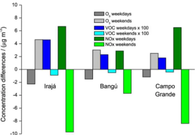
To quantitatively measure the weekend effect, the mean differences of O3, VOCs and NOx between the weekdays
and weekends were calculated for each AMS. Positive differences in the O3 concentrations and negative differences
in the O3 precursors indicated the existence of the weekend
effect in the O3. In Figure 4, it is possible to observe the
variations of the average O3, VOCs and NOx concentrations.
At the Irajá AMS, the weekend effect is more evident because of the greater differences in the O3 precursors. The
three AMS have strictly urban characteristics. However, the Bangu AMS area has a lower vehicle flow than the other two areas. Consequently, the highest O3 concentrations occurred
at the Bangu AMS because low NO concentrations resulted in low O3 consumption.
Generally, the average VOCs concentrations were lower during the weekends relative to the average concentrations during the weekdays, as observed in Figure 4. The VOC concentrations at 9:30 AM were 10.5, 17.1 and 23.7% at the Irajá, Bangu and Campo Grande AMSs, respectively. The Irajá and Bangu AMSs showed VOC concentration between 120 and 190 ppbC, and the Campo Grande AMS
registered the lowest VOC concentrations, with average concentrations of between 30 and 75 ppbC.
The VOC/NOx ratios for the weekdays and weekends
between 6:30 and 9:30 AM were calculated. Thus, the ratio during the early morning will be responsible for the ozone concentrations throughout the day. The high Irajá AMS VOC/NOx ratios resulted from the highest VOC
concentrations relative to the other AMSs. The VOC/NOx
ratios increased during the weekends because the NOx
reductions were more significant than the VOC reductions. Figure 5 shows the VOC/NOx ratios for weekdays and
weekends, which increased during the weekends at all three AMSs.
Furthermore, Ox is a photochemical indicator of O3
production and is useful because it remains unchanged throughout the formation and photo dissociation of NO2.
The Ox concentration responds better to the actual O3
photochemical production. If the Ox concentration is higher Figure 3. NOx and the NO2/NOx ratio for the AMS Irajá, Bangu e Campo
Grande.
Figure 4. Differences between O3, VOCs and NOx concentrations between
weekdays and weekends during 2012-2013 for Irajá, Bangu e Campo Grande AMSs.
on the weekdays than on the weekends, the weekend effects are generally caused by the O3 reaction with NO.
10 The O x
varied during the morning and (6:30-9:30 AM) afternoon (1:30-4:30 PM) hours, as shown in Figure 6. During both periods, greater Ox variations were observed on the
weekdays at all of the AMSs. During the afternoon hours, this difference was greater than during the morning hours, which is consistent with the occurrence of the most intense photochemical processes during the afternoon.
Particulate matter with equivalent aerodynamic diameter lower than 10 µm concentrations (PM10) were lower during the weekends, with differences of −7.7, −1.9
and −5.8% between the weekends and weekdays at the Irajá,
Bangu and Campo Grande AMSs. Although PM10 does not directly participate in the process of ozone formation, environments with higher PM10 concentrations block solar radiation due to light scattering and decrease the photochemical dissociation of NO2. This photochemical
dissociation of NO2 initiates the process of ozone formation
by forming atomic oxygen. Thus, one possible cause of the weekend effect of ozone concentrations is the reduction in PM10 concentrations during the weekend. The PM10 concentrations were evaluated during weekdays and compared with the solar radiation variations on weekdays and weekends. Lower concentrations were obtained during the weekends at the three AMSs. However, this reduction was not enough to cause a significant decrease in the average solar radiation during weekends. The average difference between the solar radiation during the weekdays and weekends was less than 0.5%. Thus, the decrease in PM10 concentrations did not cause the weekend effect at the AMSs in the city of Rio de Janeiro.
No significant differences were observed between the timing of the maximum NOx concentrations between
the weekends and weekdays. Thus, it was not possible to determine the time displacement of NOx emissions as a
possible source of the greater O3 concentrations during the
weekends. The CO concentrations were higher during the weekends than during the weekdays. Figure 7 shows the CO concentrations that occurred during the nighttime for the three AMSs. Because CO has a low reactivity and 98% of CO in the metropolitan region of Rio de Janeiro results from vehicular sources,16 it was possible to associate increases in
the concentrations with increases in vehicle emissions. This association resulted from the greater number of vehicles operating at night for leisure activities on Friday and Saturday. Similarly, higher concentrations of other primary pollutants are released on Friday and Saturday evenings and are available on Saturday and Sunday mornings to participate in the ozone formation process.
Air samples collected in 2012 and analyzed using the TO-15 U.S.EPA methodology23 are presented in Table 2.
To perform the simulations, the average VOC values were obtained for 16 samples. Some of the VOCs were grouped according to their reactivities and structures, while other VOCs were considered individually, as detailed in the SAPRAC method. Data for the criteria pollutants (CO, NOx
and HC) and meteorological parameters were processed as average values. Unfortunately, all of the VOC samples were collected during weekdays. Thus, no simulations could be performed for the weekends. The input values of criteria pollutants and meteorological parameters are described in Table 3.
After validating the model against the average CO, NOx
and O3 values from 2012 for the city of Rio de Janeiro,
the model was executed 121 times for several VOC (200 to 800 ppbC) and NOx values (20 to 160 ppb), and the
maximum ozone values were computed. These results are displayed in an isopleth graph (Figure 8).
Figure 6. Ox differences for Irajá, Bangu e Campo Grande AMS during morning hours (6:00-9:00 AM) and afternoon hours (1:00-4:30 PM) for 2012-2013.
Table 2. VOC speciation of sixteen canisters collected along the main streets of the city of Rio de Janeiro during 2012 at 6-7 AM. Values are in µg m–3
VOC Minimum / (µg m−3) Maximum / (µg m−3) Average S.D.
Formaldehyde 4.62 24.17 8.29 6.06
Isobutane 0.51 6.21 0.80 2.05
Acetaldehyde 1.00 12.39 3.12 3.53
Acetone 1.90 12.38 3.49 3.37
Propanal 0.56 7.88 1.56 2.39
1-Butene 0.59 10.59 2.33 3.14
1,3-Butadiene 0.73 9.32 2.04 2.76
Butane 8.70 30.74 12.79 6.90
Trans-2-butene 2.26 13.83 4.07 3.70
Cis-2-butene 2.44 15.91 4.79 4.23
3-Methyl-1-butene 0.92 9.50 2.18 2.77
Isopentane 10.30 37.22 15.07 8.44
Pentene 3.40 21.25 6.84 5.49
2-Methyl-2-butene 8.17 33.17 12.30 7.92
Pentane 7.30 31.25 11.49 7.53
Isoprene 0.31 7.75 1.39 2.41
Trans-2-pentene 9.53 39.56 14.72 9.45
Cis-2-pentene 3.95 23.68 7.73 6.07
1,1-Dimethylcyclopropane 13.75 52.26 20.57 12.05
2,2-Dimethylbutane 1.22 10.32 2.56 2.94
Cyclopentene 1.34 12.03 3.19 3.36
Cyclopentane 4.56 20.88 7.12 5.22
2,3-Dimethylbutane 3.11 15.41 4.99 3.96
2-Methyl pentane 13.20 48.89 19.88 11.06
Butanal 1.05 9.46 2.38 2.69
3-Methyl pentane 8.87 35.02 13.37 8.23
2-Methyl-1-pentene 0.19 8.90 1.57 2.80
Hexene 0.52 6.52 0.89 2.13
Hexane 10.21 38.32 15.04 8.85
3-Hexene 0.78 8.73 1.89 2.59
3-Methyl-2-pentene 0.28 7.05 1.22 2.21
Methylcyclopentane 5.20 21.34 7.94 5.10
4-Methyl-2-pentene 0.72 8.31 1.90 2.43
Benzene 7.90 30.17 12.42 6.81
Cyclohexane 0.68 8.44 1.93 2.47
2-Methyl hexane 0.59 8.06 1.73 2.39
2,3-Dimethylpentane 0.23 6.85 1.09 2.18
3-Methyl hexane 0.90 9.29 2.08 2.73
Cis-1,3-dimethylpentane 0.15 6.60 0.98 2.12
Heptane 0.60 8.16 1.71 2.44
Methyl cyclohexane 0.34 7.15 1.28 2.22
Toluene 12.05 42.16 17.74 9.34
2-Methyl-heptane 0.12 6.60 0.96 2.14
3-Methyl-heptane 0.12 6.51 0.95 2.10
Ethyl benzene 2.75 15.23 4.79 3.96
Benzaldehyde 1.28 10.23 2.65 2.87
p-Xylene 5.35 23.13 8.46 5.58
m-Xylene 6.20 26.07 10.19 6.08
Styrene 2.03 12.28 3.74 3.24
o-Xylene 5.20 21.64 8.13 5.15
Nonane 0.31 7.17 1.22 2.25
VOC Minimum / (µg m−3) Maximum / (µg m−3) Average S.D.
Propyl benzene 0.54 7.81 1.53 2.38
1-Ethyl-4-methyl benzene 1.00 9.24 2.16 2.68
1-Ethyl-3-methyl benzene 0.72 8.37 1.81 2.48
1,3,5-Trimethyl benzene 0.78 8.84 1.89 2.63
1-Ethyl-2-methyl benzene 0.52 7.91 1.56 2.40
1,2,4-Trimethyl benzene 1.34 10.38 2.70 2.91
Decane 0.36 7.47 1.31 2.33
1,2,3-Trimethyl benzene 0.56 7.94 1.65 2.38
Indane 0.39 7.42 1.37 2.29
1-Methyl-3-propil benzene 0.50 7.59 1.48 2.31
4-Ethyl 1,2 dimethyl benzene 0.50 8.19 1.62 2.49
Naphthalene 0.42 7.64 1.42 2.35
Undecane 0.12 6.58 0.96 2.13
Total VOC 197.10 628.80 275.90 134.50
VOC: volatile organic compounds; S.D.: standard deviation.
Table 2. VOC speciation of sixteen canisters collected along the main streets of the city of Rio de Janeiro during 2012 at 6-7 AM. Values are in µg m–3 (cont.)
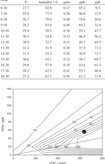
Table 3. Criteria pollutants and meteorological average hourly values for weekdays of 2012
Hour Temperature /
°C
Relative humidity / %
CO / ppm
NOx / ppb
O3 / ppb
6:30 23.7 82.8 0.47 95.2 9.5
7:30 25.0 77.3 0.56 96.6 12.9
8:30 26.7 70.0 0.48 78.6 20.6
9:30 28.2 63.6 0.40 64.2 31.4
10:30 29.4 58.5 0.36 55.1 43.7
11:30 30.3 54.8 0.33 46.9 56.2
12:30 30.9 52.7 0.31 40.7 65.5
13:30 31.2 51.9 0.30 37.9 71.2
14:30 31.1 52.2 0.30 36.9 72.7
15:30 30.6 54.1 0.31 38.7 69.7
16:30 29.6 57.8 0.35 43.6 61.3
17:30 28.3 62.5 0.42 53.1 46.8
18:30 27.2 67.1 0.50 62.2 31.9
Figure 8. Ozone isopleth plot for different VOC and NOx scenarios for the city of Rio de Janeiro.
The dependence of O3 production on the initial VOC
and NOx concentrations is frequently represented by the
means of an ozone isopleth diagram and is very particular for each city or region. The black circle shown in Figure 8 displays the actual average condition for the city of Rio de Janeiro. This region indicates that a reduction in the NOx
concentration will result in an increase in the ozone levels, as demonstrated previously. This NOx reduction results
from a reduction in the circulation of trucks and buses, with the main sources of NOx operating during the weekends.
The region over the diagonal line is a typical region where the air quality is controlled by VOC, with the exact actual conditions of Rio de Janeiro and other Brazilian cities.3
Conclusions
In the city of Rio de Janeiro, high ozone concentrations represent the main air pollution problems and have resulted in several air quality standard exceedances. The Bangu, Irajá and Campo Grande AMSs showed the greatest number of exceedances during 2012 and 2013. The largest number of air quality standard exceedances occurred during weekends.
The ozone concentrations increased by 7.30, 6.8 and 3.4% at the Irajá, Campo Grande and Bangu AMSs, respectively. All of the primary pollutant concentrations decreased over the weekends, which indicated that a reduction in vehicle emissions occurred over the weekends. The three evaluated AMSs in this study were influenced by vehicle emissions, with no significant influences from stationary sources.
When using the simulation tool in the city of Rio de Janeiro, it was observed that the ozone levels were controlled by VOCs. Thus, the NOx emissions were reduced
and freight transport on the weekend, which led to greater ozone levels.
Acknowledgements
The financial support from the Rio de Janeiro Foundation for Research Assistance (FAPERJ), Brazilian National Council for Scientific and Technological Development (CNPq) and Rio de Janeiro Municipal Environmental Agency (SMAC).
References
1. Arsic, M.; Nikolic, D.; Djordjevic, P.; Mihajlovic, I.; Zivkovic, Z.; Atmos. Environ. 2011, 45, 5716.
2. World Health Organization (WHO); Health Risks of Ozone from Large-Range Transboundary Air Pollution,Regional Office for
Europe: Copenhagen, 2008.
3. Seinfeld, J. H.; Pandis, S. N.; Atmospheric Chemistry and Physics From Air Pollution to Climate Change; John Wiley &
Sons: New York, 1999.
4. Finlayson-Pitts, B. J.; Pitts Jr., J. N.; Chemistry of the Upper and Lower Atmosphere: Theory, Experiments, and Applications,
Academic Press: New York, 2000.
5. Heuss, J. M.; Kahlbaum, D. F.; Wolff, G. T.; J. Air Waste Manage. Assoc. 2003, 53, 772.
6. Kansal, A.; J. Hazard. Mater. 2009, 166, 17.
7. Seguel, J.; Rodrigo, M. R.; Leiva, M.; Environ. Pollut. 2012, 162, 72.
8. Parrish, D. D.; Singh, H. B.; Molina, L.; Madronich, S.; Atmos. Environ. 2011, 45, 7015.
9. Gao, H. O.; Niemeier, D. A.; Transp. Res. D 2007, 12, 83. 10. Sadanaga, Y.; Shibata, S.; Hamana, M.; Takenaka, N.;
Bandow, H.; Atmos. Environ. 2008, 42, 4708.
11. California Air Resources Board (CARB); The Ozone Weekend Effect in California, Draft Staff Report and Technical Support
Document, California Air Resources Board: Sacramento, 2001. 12. Yarwood, G.; Stoeckenius, T. E.; Heiken, J. G.; Dunker, A. M.;
J. Air Waste Manage. Assoc. 2003, 53, 864.
13. Filella, I.; Peñuelas, J.; J. Atmos. Chem. 2006, 54, 189. 14. Khoder, M. I.; Environ. Monit. Assess. 2009, 149, 349. 15. Viras, L. G.; Environ. Monit. Assess. 2001, 80, 301.
16. Martins, E. M.; Machado, M. C. S.; Almeida, J. C. S.; Arbilla, G.; Bull. Environ. Contam. Toxicol. 2007a, 78, 304. 17. Martins, E. M.; de Oliveira, K. M. P. G.; Arbilla, G.; Gatti, L.
V.; Bull. Environ. Contam. Toxicol. 2007b, 79, 237.
18. http://www.denatran.gov.br/download/frota/Frota_Por_UF_e_ Tipo_DEZ_2014.rar accessed in January 2015.
19. Conselho Nacional do Meio Ambiente (CONAMA); Sets Standards of Primary and Secondary Air Quality and Even the
Criteria for Acute Episodes of Air Pollution, Resolution No. 03
of June 28, 1990; Official Journal of the Federative Republic of Brazil: Brasilia, DF, Brazil, 1990.
20. Notario, A.; Bravo, I.; Adame, J. A.; Díaz-de-Mera, Y.; Aranda, A.; Rodríguez, A.; Rodríguez, D.; Atmos. Res. 2013, 128, 35.
21. Itano, Y.; Bandow, H.; Takenaka, N.; Saitoh, Y.; Asayama, A.; Fukuyama, J.; Sci. Total Environ. 2007, 379, 46.
22. Shiu, C. J.; Liu, S. C.; Chang, C. C.; Chen, J. P.; Chou, C. C. K.; Lin, C. Y.; Young, C. Y.; Atmos. Environ. 2007, 41, 9324. 23. United States Environmental Protection Agency (US EPA);
Determination of Volatile Organic Compounds (VOCs) in Air
Collected in Specially-Prepared Canisters and Analyzed by Gas
Chromatography/Mass Spectrometry (EPA/625/R-96/010b); 2nd
ed.; Compendium Method TO-15A; Center for Environmental Research Information: Cincinnati, OH, USA, 1999.
24. Souza, C. V.; Corrêa, S. M.; Atmos. Environ. 2015,103, 222. 25. United States Environmental Protection Agency (US EPA);
Determination of Formaldehyde in Ambient Air Using
Adsorbent Cartridge Followed by High Performance Liquid
Chromatography (HPLC) (EPA-625/R-96/010b); Compendium
Method TO-11A; Center for Environmental Research Information: Cincinnati, OH, USA, 1997.
26. Corrêa, S. M.; Arbilla, G.; Atmos. Environ. 2005, 39, 4513. 27. Gery, M. W.; Crouse, R. R.; User’s Guide for Executing OZIPR,
EPA-9D2196NASA; US Environmental Protection Agency, Research Triangle Park: North Carolina, USA, 1990. 28. Tonnesen, G. S.; User’s Guide for Executing OZIPR, Version
2.0, U.S.EPA: North Caroline, USA, 2000.
29. Teixeira, J. R.; Souza, C. V.; Sodré, E. D.; Corrêa, S. M.; J. Braz. Chem. Soc. 2012, 23, 496.
30. Orlando, J. P.; Alvim, D. S.; Yamazaki, A.; Corrêa, S. M.; Gatti, L. V.; Sci. Total Environ. 2010, 408, 1621.
31. Garcia, L. F. A.; Corrêa, S. M.; Penteado, R.; Daemme, L. C.; Gatti, L. V.; Alvim, D. S.; J. Braz. Chem. Soc. 2013, 24, 375. 32. Carter, W. P. L.; Atmos. Environ. 1990, 24, 481.
33. Carter, W. P. L.; Atmos. Environ. 1995, 29, 2513.
34. Carter, W. P. L.; Documentation of the SAPRC-99 Chemical Mechanism for VOC Reactivity Assessment, Final Report to
California Air Resources Board, Contract 92-329 and Contract 95-308, 2000.
35. Carter, W. P. L.; Luo, D.; Malkina, I. L.; Environmental Chamber Studies for Development of an Update Photochemical
Mechanism for VOC Reactivity Assessment, Final Report to the
California Air Resources Board, Contract 92-345, 1997. 36. Carter, W. P. L.; Lurmann, F. W.; Atmos. Environ. 1991, 25,
2771.
37. Carter, W. P. L.; Atkinson, R.; Int. J. Chem. Kinet. 1996, 28, 497.
Submitted: May 29, 2015