Mat. Res. vol.3 número3

Kinetics of Phase Change

A.C. Faleiros

, T.N. Rabelo

, G.P. Thim

, M.A.S. Oliveira

a

Departamento de Matemática, Instituto Tecnológico de Aeronáutica, 12228-900 São José dos Campos - SP, Brazil

b

Departamento de Química, Instituto Tecnológico de Aeronáutica, 12228-900 São José dos Campos - SP, Brazil

Received: March 30, 2000; Revised: August 17, 2000

The kinetic model for change of phases developed by M. Avrami at the end of the thirties has been used to describe the temporal behavior of phase changes. Until today this model is studied and adapted to include broader hypotheses. However, the mathematical format pre-sented by M. Avrami is difficult to be understood by beginners. The purpose of this work is to clarify the mathematical treatment of Avrami’s work, going straightforward to the arguments that led to his main results.

Keywords:Avrami, phase change, kinetic model

1. Introduction

Sixty years has passed since a theory about the kinetic of the phase change was proposed by Melvin Avrami at the end of the thirties1,2. Despite of all this elapsed time, it is still used to describe the nucleation and growth of new phases3-8and new improvements have been suggested to make its hypothesis as broad and flexible as possible9-13.

Avrami’s model assumes that the system subjected to the phase change is composed by germs of the new phase. These germs are transitory molecule arranges randomly distributed that are similar to those existent in the new forming phase. According to the statistical fluctuation, these arrangements form and disappear, but some remain in latent state without growing. When, for some reason, the phase change begins, some of these primordial germs start growing, reaching a critical size and become stable. From this point on, they are called grains of the new phase. They will suffer an expansion process, at which the number of essential germs decreases with time. This decrease occurs by two mechanisms: germ transforms into grains, or grow-ing grains swallow some of the existent germs. Avrami developed his theory making these physical assumptions and doing a mathematical treatment, which considers the functional relation between the number of germs and the volume of the new growing phase.

The goal of this work is to clarify the mathematical arguments used by Avrami in his original papers, going

directly to the arguments that lead us into the main results of his theory.

2. Germs, Grains and Transformed Volume

In this section the notation and the basic principles of Avrami’s model will be established.

Consider a metastable material that starts changing phase at some moment. LetN0be the number of essential germs of the new phase per unit volume at the beginning of the phase change process. Germs form and disappear but it can be supposed that their density remains constant during the phase change process.

Two mechanisms can be considered to explain the temporal variation of the number of germs. In the first one, germs start growing and become grains of the new phase. In the second one, germs are swallowed by the growing grains, which occupy the places before occupied by the swallowed germs. In the following paragraphs the kinetic of these two mechanisms will be described.

For the first mechanism, letN=N(t)be the number of germs for the new phase per unit volume at the instantt

Suppose uniform distribution of the germs in the entire volume of the previous phase. At the initial time,N(0) =N0. LetN’=N’(T)be the number of grains of the new phase, at the instanttper unit volume. The probabilitynof a germ to transform into grain, per unit of time, is given by the equation14-19

e-mail: faleiros@ief.ita.cta.br

n=n(T) =Ke−

[Q+A(T)]

RT

Here, Q is the activation energy per mol, T is the absolute temperature, R is the universal constant of the gases, andA(T) is the necessary work to form a mol of grain at the temperatureT. Therefore, the variation of the number of germs that transform into grain per unit volume at the time perioddtis given by

dN’=nN dt

For the second mechanism, the variation in the number of germs is due to the new phase growth that, by expansion, swallows the germs and occupies the places before occu-pied by the swallowed germs. LetN”=N”(t) be the number of swallowed germs per unit volume at the instantt. The variation of the number of swallowed germs per unit vol-ume at the time perioddtis given by

dN’’=N0dV

here,dVis the volume variation per unit volume of the new phase during the time perioddt. However, this is an roughly estimated relation, which is applied when the number of grains is small in relation to the number of germs. In a future section we will present the exact relation for the swallowed germs.

The variation of the number of germs per unit volume at the time period is given by

dN=−dN’−dN’’

The negative sign is justified by the fact that an increase of N’ andN” produces a decrease of N. Therefore, the derivatives ofN,N’andN”, per unit volume at the instant

tare

dN dt = −

dN’

dt − dN’’

dt (1)

dN’

dt =nN (2)

dN’’

dt =N0 dV

dt (3)

One important particular case for the Eq. 1 happens whennis so big that almost all germs transform into grains before any ingestion has the chance to occur. In this case, the termdN”/dtcan be ignored in comparison with the term

dN’/dtand Eq. 1 reduces to

dN dt = −

dN’

dt = −nN (4)

If the temperature and the essential germ concentration remain constant,n can be considered constant during the entire process and, under these conditions, Eq. 4 becomes

a separable differential equation. Dividing (4) by N it follows

1 N

dN dt =−n

or

d

dt[lnN(t)]= −n

Integrating it from the initial time to the timet,

lnN(t)−lnN(0) = −nt

or

ln[N(t)

N0]= − nt

and, explicittingN(t),

N(t) =N0e−nt (5)

Taking the above equation to Eq. (4), and integrating it, follows

N’=

∫

t

dt=

∫

t

e−ntdt=nN0

∫

t e−ntdt

or

N’=N0(1−e−nt)

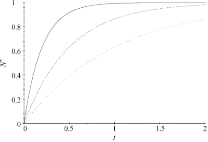
whereN’→N0whent→ ∞. Figure 1 shows the curves for

N’=N0(1−e−nt)

withn= 1, 2, and 5 andN0= 1.

3. Characteristic Time Scale

Going back to the general case, to simplify Eqs. 1, 2 and 3, another time scaleτ = τ(t) defined by

52 Faleiroset al. Materials Research

Figure 1.Curves for N’=N0(1−e−nt), withn= 1, 2, and 5 andN0= 1.

τ=

_∫

t

will be used. Its derivation in the variabletproduces

dτ

dt (t) =n(t) (6)

The relation between the time scale t and τ will be uniform only ifnis constant during the entire process. This new time scale is called characteristic time scale. From this point on, unless opposite mention, the characteristic time τ will be used. As n > 0 the derivativedτ/dt = n will be positive, assuring thatτ = τ(t) is strictly increasing having, in this way, an inverset=t(τ) The derivative of this inverse is

dt dτ=

1

n

Substituting Eqs.(2) and (3) in Eq. (1), the following is obtained:

dN dt =−

dN’

dt − dN’’

dt = −nN−N0 dV

dt

and, changing it to the variableτ,

ndN

dτ =−nN−N0 dV dτ

or

dN

dτ +N+N0 dV

dτ =0

Integrating the above equation from 0 toτ, follows

N(τ)−N(0) +

∫

τ

+N0[V(τ) −V(0)]=0

and, sinceN(0) =N0andV(0) = 0,

N(τ)−N0+

∫

τ

+N0V(τ) =0 (7)

To solve this integral equation, it is necessary to obtain the functional relationV(τ), which is a composite function similar toϕ(t(τ)) that can be rewritten as

ϕ (τ) = ϕ(t(τ)) = ϕ(t)

whent=t(τ). The chain rule applied to this function can be written in the following way

dϕ dt =

dϕ dτ

dτ dt=

dϕ dτn=n

dϕ

dτ (8)

Applying the Chain rule (8) to Eq. (2), follows

dN’

dτ =N (9)

which can be integrated. As N’(0) = 0, this integration results in

N’(τ) =

∫

τ

(10)

Equation (7) is valid only during the time that there are germs to be consumed or to be transformed into grains. Let

t = t or τ = τ be the instant in which all germs were consumed. From this time on, the number of grains remain constant. While the numbersNandN’and remain constant, the volume of the new phase keeps growing.

4. Exact Relationship for the Swallowed

Germs

In this section we will improve the description for the

N’(t) behavior.

We must observe that Eq. (3) is valid when the number of grains is small in comparison with the number of germs. Otherwise, the density found by the new phase progressive front isN/(1 -V) where (1 -V) is the volume fraction per unit volume that was not transformed. Thus, when the number of grains is not small compared with the number of germs, Eq. 3 must be substituted by

dN’’= N

1−VdV (11)

which taken to Eq. (1) gives

dN

dt = −nN− N

1−V dV

dt

or, in theτvariable

ndN

dτ =−nN− nN

1−V dV dτ

Dividing the above equation bynNfollows

1 N

dN dτ = −1−

1 1−V

dV dτ

or

d

dτ(lnN) = −1+ d

dτln(1−V)

whose integral from 0 toτleads to

lnN−lnN0= −τ +ln(1−V)

that can be solved in the variableNproducing

Substituting Eq. (12) in (10) results into

N’(τ)=N0

∫

0

τ

(13)

According to Eq. (12),Ndecreases asymptotically to zero but doesn’t vanish. However, experiments show that at certain instant τ the germs exhaust. To describe this experimental fact, it must be observed that Eq. (13) is valid only until the instantτ. In order to have agreement between experimental results and theory, it is necessary to attribute a defined value toτfor small values ofN. We can arbitrarily makeτequal to the instant in whichN= 1 and take this value to Eq. (12), which follows

N=1=N0e−τ

_

[ 1−V( τ

_ )]

This is a transcendental equation definingτ

For τ bigger than τ, N is practically null, while N’

remains constant with values given by Eq. 13

N’(τ)=N’(τ

_

) =N0

∫

τ _

5. Extended Volume

In this section, to obtain the functional relationV[N(τ)] between the transformed volume and the number of grains, it is developed the concepts of averaged radius and volume of the grain. From these concepts the extended volume of the new phase is obtained. This relation is necessary in order to integrate Eq. (7).

Not all grains start growing at the same instant. When a grain touches another one, there is an interruption in its growth at the interface. The volume that a grain would have if its growth were not interrupted by the contact with another grain is calledextended volume. The grain that was born at instantzhas, at the momentτ, an extended volume represented byvex(τ, z). Both instants are referred to the

characteristic time scale.

Generally, the grains are not perfectly spherical. There-fore, when one refers to the radiusrof a grain, in fact, we are referring to the averaged radius of the grains. The radius that a grain would have if there were not contact among the grains is called extended averaged radius. LetG(t) be the averaged rate of growth of a grain. At an instant t the extended averaged radius of a grain, which was born at the instantt=yis given by

rex(t,y)=

∫

t dt’

In the characteristic time scale, this extended radius of the averaged grain is

rex(τ,z) =

∫

t

dt’=

∫

τ

τ’)dt’ dτ’dτ’=

∫

G(τ’)

n(τ’) z

τ

dτ’

or

rex(τ,z) =

∫

τ

(τ’)dτ’ (14)

where

α(τ’)=G(τ’) n(τ’)

Here, τ= zis the instant that a grain appeared. The extended volume of the grain is

vex(τ,z)= σr3=σ[

∫

0

τ

dτ’ ]3 (15)

whereσis a shape factor, equal to 4π/3 for spherical grains. LetdN’(z) be the variation of the number of germs that transform into grains between the instantsτ=zandτ=z+

dz. According to Eq. 9,dN’(z) =N(z)dz. If the volume of each grain were added, supposing that the growing of each grain is not hinder by other grains, we obtain the total extended volume per unit volume at the instantτ

Vex(τ) =

∫

0

τ

(τ,z)dN’

dz(z)dz=

∫

τ

(τ,z)N(z)dz (16)

6. Characteristic Phenomena at the

Isokinetic Phase

The factors that controlnmust controlGand it might be expected similarities between the variation of these parameters with the external conditions. Keeping this in mind, one can infer thatnandGare approximately propor-tional at a large range of concentration and temperature. This range will be calledisokinetic range. If one admit that the relation

α =G

n

is constant for a given substance at the isokinetic range, from Eqs. (14) and (15) we obtain

r= α (τ −z) (17)

vex(τ,z) =σ α3(τ −z)3 (18)

and from Eq. (16),

Vex=

∫

0

τ

(τ,z)N(z)dz=

∫

0

τ

α3_N(z)dz=

σα3

∫

0

τ

τ−z)3N(z)dz (19)

Ifαis independent of the temperature and concentration at the isokinetic range, the transformation story and the kinetic description of the process at the time scaleτwill also be independent of the temperature and concentration. Therefore, for a given substance, there is an isokinetic range of temperature and concentration, at which the charac-teristic kinetic of a phase change remains unaltered at the characteristic time scale. Thus, to establish the kinetics of a reaction in a concentration and temperature range at the isokinetic range, it is enough to solve just one problem at the time scaleτ.

Equations (15), (18) and (19) apply to pseudo-spherical or polyhedral grain growth. If the grain grows along two or one dimension (plate or needle like), Eq. (19) must be substituted by

Vex= σ’α2

∫

0

τ

τ −z)2N(z)dz (20)

and

Vex= σ’’α

∫

0

r

τ −z)N(z)dz (21)

where σ’ =πandσ” = 1. Equation (19) applies only to isokinetic domains, i.e., in the situations that α= G/n is constant.

7. Evolution of the Extended Volume

In this section Avrami’s main argument is developed. Letzbe the instant in which the grain appears andτthe actual time of the phase change, both in the characteristic time scale. Consider a grain, selected arbitrarily, and let

v’ =v’(τ, z) be the volume part of this grain that is not superimposed to other grains and vex = vex(τ, z) be the extended volumeof this grain,i.e., the volume that it would have if its growth were not obstructed due to the contact with other grains. If this grain were taken off from its place, leaving behind the overlapped parts,v’ would be the frac-tion matter not transformed, which during the phase change contributed exclusively for this grain growth. Therefore,

v’/vexis equal to the volume fraction of matter that remains

in the old phase. Remembering that 1 -V(τ) is the volume fraction that was not transformed, it follows that, on aver-age,

v’

vex=1−V (22)

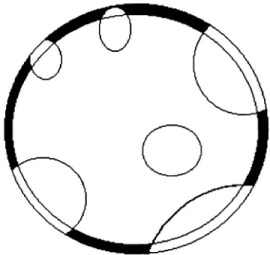
Another way to justify this equation is the following: If, for example, 30% of the initial volume is transformed, it follows that (1 -V) = (1 - 0,3) = 0.7. Analyzing a grain in this medium, on average, 30% of it will be superimposed to other grains. Since vex is the extended volume of the

grain, the partv’ that is not superimposed to other grains must be equal to 70% of the extended volume andv’/vex

must be equal to 0.7. Figure 2 depicts a grain with extended volumevexand its part with volumev’.

Admitting grains randomly distributed, Eq. (22) can be used as an average. However, the grains are randomly distributed only in the region that was not transformed. In the transformed region, there are only grains of the new phase and all germs were swallowed. Therefore, the as-sumption that the grains are randomly distributed is true only for grains that, at the timezof its appearance, were outside of the transformed volumeV(z). There are two ways to overcome this situation and obtain the same final result. The first way to overcame the situation mentioned above is to consider all germs, including those that, at the instant z, are located inside of the grains, which will be called ghost germs. The number of these germs, in the characteristic time scale, is given by Eq. (5)

N(z)=N0e−z

In this case, the random situation can be reestablished if we associate ghost grains to those germs that would be transformed into grains if they had not been absorbed by the other grains that grew up. During the time interval from

zto (z+dz), the variation of the number of new grains per unit volume, including the ghost grains, isdN’(z) =N(z)dz, whereN(z) =N0e-z. Ifvex(τ, z) is the extended volume of

Vex(τ)=

∫

0

τ

(τ,z)dN’(z) =

∫

0

τ

(τ,z)N(z)dz=

N0

∫

τ

vex(τ,z)dz (23)

Consider the following property of real numbers: if

x1 y1=

x2 y2= … =

xk yk=

L

then

x1+x2+… +xk y1+y2+ …+y3

=L

Taking into account this property, and adding the nu-merators and denominators of Eq. (22) over all grains, we obtain

V’

Vex=1− V

whereV’ is the overall grain addition ofv’ whileVexis the

overall grain addition ofvex

From the above equation and Eq. (23),

V’

1−V=Vex=N0

∫

−z_v

ex(τ,z)dz 0

τ

(24)

The second way to arrive at the above result is to assume random distribution of the germs only in the volume 1 -V(z) that was not transformed at the instantz, and consider that the number of germs in this region is expressed by Eq. (12)

N=N0e−z[1−V(z)]

In this case, when ghost grains are not considered, the

Vexvalue is still given by

∫

0

τ

=

_∫

0

τ

At the instantz, the volume that was not transformed is 1 -V(z) The germs that started growing atzwere randomly distributed in this volume. At the instantτthe volume in the old phase is 1 -V(τ). The ratio

1−V(τ) 1−V(z)

is the fraction of volume that was not transformed at the instantτin relation to the volume that was not transformed at the instantz. Since the ghost grains are not considered in this case, one can consider thatzis the initial instant of the transformation and that the initial volume of the material that did not suffer any change is 1 -V(z). Like before, in average, the ratio between v’ and vex is equal to the

volumetric fraction of matter that was not transformed. Now, this fraction is equal to [1 - V(τ)]/[1 - V(z)] and, therefore,

v’

vex

=1−V(τ)

1−V(z)

or

v’ 1−V(τ) =

vex 1−V(z)

Multiplying both sides of this equation by the number of grainsdN’(z) =N(z)dzformed during the time interval

dz, follows

v’(τ,z)N(z)dz

1−V(τ) =

vex(τ,z)N(z)dz 1−V(z)

or using Eq. (12)

v’(τ, z)N(z) 1−V(τ) dz=

vex(τ, z)N0e−z[1−V(z)] [1−V(z)] dz

which integrated from 0 toτgives

1

1−V(τ) =

∫

τ

(τ,z)N(z)dz=

∫

τ

e−zvex(τ,z)dz

But,

∫

0 τ

(τ,z)N(z)dzis exactlyV’(τ) and hence,

V’(τ)

1−V(τ) =N0

∫

−z

0

τ

vex(τ,z)dz

which coincides precisely with Eq. (24).

When the new phase is composed of thin grains, the grains superimpose very little and we can assume that

V(τ) =V’(τ) which combined with Eq. (24) gives

V(τ)

1−V(τ) Vex(τ) =N0

∫

−z

0

τ

vex(τ,z)dz (25)

Under isothermal conditions and uniform concentra-tions,ncan be considered constant. Considering polyhedral growth, at the time scaletthe extended radiusrexof grains

that appeared at the instantyis proportional tot - y. That is rex=G(t-y), where the constant of proportionalityGis the

radial growth rate. In the characteristic time scale,τ=nt

andz=nythus,rex= (G/n)(τ-z) =α(τ-z), withα=G/n.

Therefore,

vex(τ,z) =σα3(τ-z)3

whereσ= 4π/3 for spherical grains. From Eq. (25),

Vex= σ α3N0

∫

τ

τ −z)3e−zdz=

6σG3N0

n [e

−τ_{−1+τ −} τ2

2!+

τ3

3!]

or

Vex=βE3(−τ) (26)

with

β =8πN0(G n)

3

(27)

and

Em(−τ) = 1 m!

∫

τ

τ−z)me−zdz=

(−1)m+1[ e−τ−1+ τ −τ

2

2!+

…_{+ (−1)}m+1τm

m!]

Whenτ<< 1 one obtains

e−τ~_{1−τ +}τ

2

2!−

τ3

3!+

…_{+ (−1)}mτ

m

m!+

(−1)m+1 τ m+1

(m+1)!

Thatway,

e−τ−1+ τ −τ 2

2!+

τ3

3!−

…_{− (−1)}mτm m!

~

(−1)m+1 τ m+1

(m+1)!

and, therefore,

Em(−τ) ~

τm+1

(m+1)! forτ<< 1 (28)

Whenτ>> 1, the e-τvalue becomes very small,i.e., this value is much smaller than any entire power ofτ. In this case, who dictates the asymptotic behavior is the biggestτ power and hence

Em(−τ) ~

τm

m! forτ>> 1 (29)

Using the Eqs. (28) and (29) asymptotic developments in Eq. (26), one obtain

Vex= βE3(−τ) ≈

βτ4 4! = (

πG3N0n

3 )t

4

whenτ<< 1 and

Vex= βE3(−τ)~

βτ3

3! =(

4πG3N0

3 )t

3

whenτ>> 1.

Both of the equations have theBtkformat, withBandk

constants. Substituting these equations in Eq. (25), follows

V(t)

1−V(t) = Bt

k

(30)

which is the empirical expression obtained by J.B. Austin and R.L. Rickett20 for the isothermal transformation of super-cooled austenite into bainite.

Equation (26) is valid until total germs consumption, which occurs at the instant τ. From this instant on, the superior limit of the integral must be substituted by τ. In this case Eq. (26) transforms into

Vex=

β

3!

∫

τ _

τ −z)3e−zdz

Although germs do not exist anymore, the grains keep growing. This explains the appearance of τandτin this

integral. Applying the property

∫

0 τ _

=

∫

0 τ

−

∫

τ _ τ

to the above

equation, one obtain

Vex=

β

3![

∫

τ

τ−z)3e−zdz−

∫

τ

_ τ

τ −z)3e−zdz]

and makingx=z-τ,

Vex=

β

3![

∫

τ

τ −z)3e−zdz−

∫

0

τ −τ_

τ −_τ−x)3e−x−τ

_

dx]= β 3![

∫

τ

τ −z)3_e−z_dz−

e−τ

_

∫

0

τ − τ_

τ − τ_−x)3e−xdx]

From theE3(-τ) definition, one can write

Vex=β[E3(−τ)−e−τ

_

E3(− (τ −τ _

))]

In order to obtain the needle and planar growth expres-sion, it is enough substituteE3forE1andE2andβwill be nowN0(G/n) and 2πN0(G/n)2, respectively. Defining

E3(-τ) for polyhedral growth

E (τ) = E2(-τ) for planar growth E1(-τ) for linear growth

it is possible to unify the previous expressions and write, for the three growth types,

Vex=β[E(τ) −e−τ

_

E(τ − τ _

8. Relation between Real and Extended

Volume

Applying the same logic used in the previous section to the volume increment of only one grain in a small time interval, one obtain for the averaged grain

dv’

dvex

=1−V

Figure 3 depicts the meaning of the differential volumes

dv’ and dvex. Here, as we are dealing with infinitesimal

increments,dv’ =dv. Multiplying and dividing the previous ratio by the number of grains per volume, we obtain

dV dVex=1−

V (32)

which is a separable differential equation. Rearranging this equation and integrating it, it comes

ln(1−V) −lnC= −Vex

or

1−V=C e−Vex

whereCis the integration constant. Considering thatVex=

0 whenV= 0, we getC= 1 so that

V=1−e−Vex ₍₃₃₎

This is the fundamental relation, applicable to every case in which there is a randomly thin grain distribution. This deduction was made independently of isothermal or isokinetic assumptions. Using Eq. (33) into Eqs. (12) and (13), we obtain

N=N0e− (τ +Vex) (34)

N’=N0

∫

τ

dz (35)

9. Isokinetic domain transformation

The phase change kinetics is totally determined by Eqs. (33), (34) and (35). For the isokinetic case,Vexis given by

Eq. (26), which applied to Eqs. (33), (34) and (35), produces

V(τ) =1−e−βE(τ) (36)

N(τ) =N0e[−(τ + βE(τ))] (37)

N’(τ) =N0

∫

τ

dz (38)

remembering thatE(τ) =Em(-τ).

Equation (37) shows that the number of germs de-creases exponentially, but never vanishes. However, it is observed experimentally that they become equal to zero at some timeτ. This time is considered the one whenN= 1 This unit value is negligible in comparison with the initial particles number and can be considered the actual zero point. AssumingN(τ) = 1 in Eq. (37), it follows

τ _

+ βE(τ

_

) =lnN0 (39)

When τ>τ, the number of germs are exhausted. Using Eq. (31) in Eqs. (33) and (38), one obtain

V(τ)=1−e[−β(E(τ)−e−τ

_

E(τ − τ_)] ₍₄₀₎

N’(τ) =N0

∫

τ _

dz (41)

10. Beginning of the Transformation

For polyhedral growth andτ<< 1 from Eqs. (28) and (36), one obtain

V~_1−exp(−βτ 4

4!)

~₁₋₁₊βτ 4

4!

or

V~ β

4!τ

4

(42)

whereβ= 8πG3N0/n3andτ=nt.

Taking into account that

exp{-[z +βE(z)]} ~ 1

whenτ<< 1, Eq. (38) reduces to

N’(τ) =N0

∫

τ

dz~ _N 0

∫

0

τ

dz=N0τ (43)

58 Faleiroset al. Materials Research

Equation (43) shows that, at the initial instants of the transformation, the number of grains present is proportional to the time, while Eq. (42) shows that the transformed volume is proportional tot4.

Equation (42) shows that the transformation “begins” whenβτ4/4! is significantly different from zero. For usual values ofβ, this occurs whenτis around 1. Lett=tbbe the

instant at which the transformation starts. As τ=nt, we obtainntb=τb≅1 ortb= 1/n. This result was empirically

obtained by H. Krainer21in his experiments for the decom-position of austenite in steels.

11. Temporal Evolution of the

Transformation

In this section we will be concerned with obtaining relations valid during almost the entire isokinetic transfor-mation.

From the expressions (36) and (40), valid forτ < τand

τ ≥ τ, respectively, which we reproduce again:

V(τ) =1−exp(−βE(τ))

and

V(τ) =1−exp(−β[E(τ)−exp(−τ

_ E(τ−τ

_

))])

one obtain the following estimations:

1. If N0 >> 1 (situation in which the germs do not

vanish) andn<< 1 (case in whichτ<< 1 during almost the entire transformation), Eq. (42) will be a good approxima-tion during the entire transformaapproxima-tion, and one obtain the situation studied by Mehl-Johson22.

2. If N0 >> 1 (situation in which the germs do not

vanish) andn>> 1 (case in whichτ>> 1 during almost the entire transformation), Equations (36) and (29), give us

V ~_1−e−σG3N0t3 ₍₄₄₎

3. IfN0is small (the number of germs become equal to

zero at the beginning of the transformation, so thatτ<< 1), Eq. (39) together with the asymptotic development Eq. (28), give us

lnN0= τ _

+ βE(τ

_

)~τ _

+βτ

_

−m+1 (m+1)!

~ τ _

(45)

wherem= 1, 2, or 3, respectively, for needle, planar and volumetric growing. Asτis small,τ>τduring almost the entire transformation. In this way, almost the entire transformation can be described by Eq. (40). The asymptotic relation Eq. 29, valid forτ>> 1, gives

βE3(−τ)~ τ 3

3!β = β

n3t3

6 (46)

Taking the asymptotic r elations (45) and (46) to (40), andconsider ingthat(τ-τ) is almost equal toτsinceτcan be considered small, follows

V(τ) ~ _1−exp(_β[E(τ)_−exp(_−lnN

0E(τ) )]) =

1−exp(−βE(τ) (1− 1

N0 ))~

1−exp(− 6σG 3_N

0

n3

n3_t3

6 (1− 1

N0))

Here, the identity exp(-lnN0) = 1/N0 was used. After

simplifications,

V(τ)~_{1−exp(−σG}3_(N

0−1)t3) (47)

which is very similar to Eq. (44). The occurrence ofN0- 1

instead of N0 as in Eq. (44), is due to the fact that the

ultimate germ per unit volume was neglected to deduce this last equation.

Similar deductions can be done for phase changes with planar and needle growth.

For planar growth,

V=1−exp(−σ’⁄3G2N0nt3) (48)

valid whenn<< 1 and

V=1−exp(−σ’G2N0t2) (49)

valid whenn>> 1. For needle growth,

V=1−exp(−σ’’_⁄2GN0nt2₎

(50)

valid whenn<< 1 and

V=1−exp(−σ’’GN0t) (51)

valid whenn>> 1

All the above expressions have the same format of the Austin-Rickett20formula

V=1−exp(−Btk_{) (52)}

The τ value for certain level of transformation, for example 25%, or 50% or 75%, is always the same for a big range of temperature, concentration, etc. Using Eq. (36), one obtain the ratio

E(τ0.75) E(τ0.25)=

ln(1−V0.75) ln(1−V0.25)=

ln(1−0.75) ln(1−0.25)=4.82

From the asymptotic relations (28) and (29), it follows

Em(−τ0.75) Em(−τ0.25)

~₍τ0.75 τ0.25

and

Em(−τ0.75) Em(−τ0.25)

~(τ0.75 τ0.25

)mforτ>> 1

where m = 1, 2, or 3 for needle, planar or volumetric growing, respectively. From these relations it comes for

τ<< 1,

τ0.75 τ0.25

= (Em(−τ0.75) Em(−τ0.25)

)1_⁄

m+1≈_4.821⁄m+1 ₍₅₃₎

and, forτ>> 1,

τ0.75 τ0.25

~ (Em(−τ0.75)

Em(−τ0.25))

1_⁄

m~_4.821⁄m ₍₅₃₎

The asymptotic relations (53) and (54) furnish the ex-treme values between whichτ0.75/τ0.25is situated. Making

m= 3, 2, and 1, the extreme values between which the ratio

τ0.75/τ0.25 is located, for polyhedral, planar and needle growth are, respectively,

1.48≤t0.75 t0.25=

τ0.75 τ0.25≤1.69

1.69≤t0.75 t0.25=

τ0.75 τ0.25≤2.2

2.2≤t0.75 t0.25=

τ0.75 τ0.25≤4.82

Here, the approximations (4.82)1/4= 1.48, (4.82)1/3= 1.69 and (4.82)1/2= 2.2 were used.

Several experimental results fall inside the above inter-vals23. Some discrepancies were observed and need to be analyzed to obtain better understanding of the factors that provoked these deviations.

12. Conclusion

The analysis done in this work shows, step by step, the kinetic model proposed by M. Avrami to describe the kinetics of phase change.

A different model to visualize de most important part of Avrami’s arguments is proposed (Evolution of the ex-tended volume), which we consider easier to understand than the ones proposed before.

The final result of the model is the fundamental relation:

V=1−exp(−B tk)

which is applicable to every isokinetic and isothermal phase change transformation. Fitting experimental results with

this expression, one determine the values ofBandkfor the kinetic law of a phase change.

The model also makes possible to determine the dimen-sion of the grain. This can be done utilizing the ratio between two growth time. For example, take the spent time to 75% of a new phase grow in relation to the one necessary to 25% of the new phase grow. After that, compare the value for this ratio with the ones predictable by the asymptotic relations (53) and (54), which furnish the extreme values for τ0.75/τ0.25 for polyhedral, planar and linear growth, respectively.

References

1. Avrami, M.J. Chem. Phys., v. 7, p. 1103, 1939. 2. Avrami, M.J. Chem. Phys., v. 8, p. 212, 1940. 3. Weiberg, M.C.; Birnie, D.P.; Shneidman, V.A. J.

Non-Crystalline Solids, v. 219, p. 89, 1997.