Abstract
Two-dimensional motion of a rope fixed at one end is consid-ered. The Rigid Finite Element Method (RFEM) is reviewed and applied to obtain a model of the rope, including its elastic and dissipative properties. Equations of motion are derived without the small displacement assumption, using the Lagrange equations. The resulting model is compared to another one, being derived within the framework of standard analytical me-chanics methods and the Lagrange formalism. Advantages of the RFE approach are discussed from a computational point of view. The presented, alternative model can be a basis for e cient numerical simulations, which seem to be useful in further, comparative studies of the rope dynamics.
Keywords
Application of the rigid finite element method to modelling ropes
1 INTRODUCTION
Using discrete models to approximate continuous systems is a common procedure. It can be ex-tremely convenient when dealing with mechanics of a deformable solid body submitted to large displacements and deformations, e.g. ropes, cables or belts. A discrete model may be produced by applying various theoretical formulations. The slender bodies, for instance, can be simply repre-sented as chains of rigid elements and described with use of some analytical mechanics methods. Otherwise, the discretization may be an imminent feature of a certain computational technique, e.g. the Finite Element Method (FEM). The former approach has been previously applied to de-scribe and simulate motion of a hanging rope (see [1{3]). However, the resulting mathematical model consists of the implicit system of ordinary differential equations (ODEs):
( ) ( , , )t
M q q f q q (1)
with time-dependent mass matrix on the left-hand side. Consequently, numerical integration is a cumbersome process, involving very sophisticated strategies. The difficulties can be avoided when using the Rigid Finite Element Method (RFEM).
Henryk Kaminski, Pawel Fritzkowski
Henryk Kaminski, Ph.D.: Poznan University of Technology, Institute of Applied Mechanics, Piotrowo 3,
60-965 Poznan, Poland ([email protected]).
Pawel Fritzkowski, M.Sc.: Poznan University of Technology, Institute of Applied Mechanics, Piotrowo 3, 60-965 Poznan, Poland
This method was developed by Kruszewski et al. [4] and should be distinguished from the clas-sical FEM. In the RFE approach, a phyclas-sical model is composed of rigid (nondeformable) bodies connected by massless elastic-dissipative elements. In this paper, the methodology is outlined and employed in modeling of the rope. Perhaps the earliest studies of the rope motion were done by D. Bernoulli (1732) and Euler (1781). They considered and solved the problem of small vibrations of a perfectly flexible, uniform rope which is fixed at one end [6]. Nowadays many researchers derive and improve models of various slender bodies. Usually continuum approach is applied, e.g. in case of ropes [10, 13], cables [9], y lines [7] and even chains [10, 11]. Probably dynamics of a whip is most spectacular, which has been investigated both theoretically and experimentally. The contemporary theory of whip motion was developed by Goriely and McMillen [8]. When it comes to a discrete approach, the chain-like model of Pieranski and Tomaszewski [12] should be men-tioned, which was crucial for our previous works on the classical problem of rope dynamics.
2 PHYSICAL MODEL
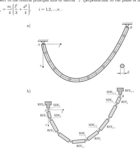
The RFE approach has been thoroughly described in [4, 5]. Let us consider a rope of length L and mass M which is initially suspended between two supports (see Fig. 1a). Physical model of the system is created in two steps. First, the slender body is divided into ñ sections of equal length
/
l L n. Elastic-dissipative properties of each section are concentrated in its center and
rep-resented by a spring-damping element (SDE). Due to the secondary division, the system consists of n ñ 1 rigid finite elements (RFEs) interconnected, and connected to foundation, via the SDEs as illustrated in Fig. 1b. The SDEs are assumed to be massless and characterized by stiffiness and damping coefficients. Every RFE, in turn, is described by mass and inertial mo-ments.
The two additional rigid elements (RFE0 and RFEn+1) can be regarded as a foundation or can
be used for realization of non-stationary constraints (movable supports). The classical fall of a folded rope can be observed as the parameters of SDEn+1 have zero values.
3 MATHEMATICAL DESCRIPTION
In case of the plane system, every RFE has three degrees of freedom and its position can be speci-fied with use of the generalized coordinate vector qi qxi,qyi,q i T. As illustrated in Fig. 2,
there is a local coordinate system ix yi connected to the ith rigid element. However,
note that qi related to the global, reference system xy. Similarly, the generalized forces acting on
the RFE can be specified by the vector Pi P P Pxi, yi, i T.
Assuming that the rope is a homegenuous prismatic bar of diameter d, length of the RFEs can be written as l1 ln l/ 2 and li l for i 2, 3, ,n 1.Consequently, the mass
/ , 1,2, ,
i i
re-spect to the central principal axis of inertia iz (perpendicular to the plane of motion) is given by
2 2
, 1,2, ,
4 3 4
i i
i
m l d
J i n .
a)
b)
Fig. 1 Division of a rope: a primary division into equal segments, b secondary division: RFEs connected by SDEs
The system has N = 3n degrees of freedom. In the RFE approach, equations of motion are derived using the Lagrange equations:
d
, d
T T D V
t q q q q P (2)
where T denotes kinetic energy of the system, V is potential energy of the system, D is the dissipation function. The vectors q and P are composed of the subvectors qi and Pi, respective-ly: 1 1 2 2 , , n n q P q P q P q P (3)
The first two terms of Eq. (2) have the form:
, d
d
T T
t q q A q (4)
where A is a diagonal mass matrix (N N ), defined as
3 2, 1,2, ,
3 1, 1,2, ,
3 , for for
for 1,2, ,
i
i
i kk
k i i n
k i i
m
J n
m
n k i i
A (5)
Now, consider two neighbouring RFEs (see Fig. 3). The ith SDE is assumed to have the same orientation as the ith RFE. Deformation of the SDEi can be written as follows:
1 1 1 1 1 1 1 , i i Ai Bi xi i i
i yi Ai Bi
i i i
x x
w
w y y
w q q
w (6)
where position of the points Aiand Bi 1 are expressed in the same coordinate system; the
subscripts x, y, correspond to tension, shearing and bending, respectively. The potential
en-ergy and the dissipation function of the system become
1
2 2 2
1 1
1
, 2
n n
xi xi yi yi i i i xi
i i
1
2 2 2
1 1
. 2
n
xi xi yi yi i i
i
D B w B w B w (8)
In the above formulas Cxi, Cyi, C i are stuffiness coefficients and Bxi, Byi, B i are damping coefficients, which can be expressed as follows [4]:
, , ,
xi yi i
EA GA EI
C C C
l l l (9)
, , ,
xi yi i
A A I
B B B
l l l (10)
where A denotes the cross-sectional area of the rope, I is the second area moment of the rope's cross-section, E denotes the Young's modulus, G is the shear modulus, denotes the shape fac-tor, and are material constants of normal and tangential damping, respectively. Unlike in the case of small vibrations, wi and wi have much more complex forms and the derivatives
/
V q and D/ q cannot be linearly expressed in terms of qand q. Finally, the equations of motion are given by
( , , ) ,t
A q F q q (11)
where F is a non-linear vector function, including the components resulting from spring de-formation, gravity, dissipation and external forces. Considering that A is diagonal, Eq. (11) can be easily transformed to
(t, , ) .
q F q q (12)
Compared with Eq. (1), the mathematical model (12) is a system of ordinary differential equa-tions in the standard (explicit) form. Therefore, solving initial values problems for the equaequa-tions seems to be significantly simpler and straightforward: many sophisticated techniques, necessary in the former case (especially for computation and processing of the left-hand side matrix), become redundant. Using an appropriate solver can lead to very efficient numerical simulations, which plays a crucial role in studies of long-term behaviour of physical systems (e.g. in chaos identifica-tion).
4 NUMERICAL EXPERIMENT
To verify the numerical efficiency of the presented approach, a series of simple numerical experi-ments have been performed with use of two different models and the results have been compared. Consider motion of the rope which is initially deflected aside, which means that the deflection angle is equal for all the rigid elements: q i(0) , where i 1,2,...,n and 75º. Parameters
of the rope are presented in Tab. 1. It should be noticed that the damping material constants fulfil the relation [4, 5]:
. G
E (13)
Quantity V alue U nit
Rope density, 6000 kg/m3
Rope length, L 1.0 m
Rope diameter, d 0.005 m
Young’s modulus, E 35 10 6 Pa
Shear modulus, G 14 10 6 Pa
Material constant of normal damping, 103 Ns/m2 Material constant of tangential damping 4 10 2 Ns/m2
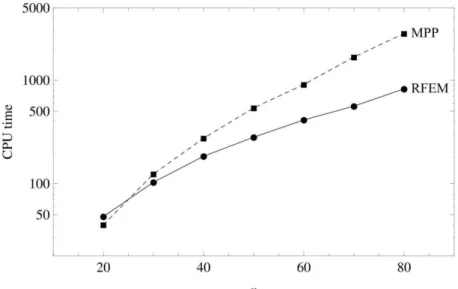
The problem of the rope dynamics has been solved several times for different discretization density. More precisely, the number of RFEs and the number of the pendulum members have been varied. As with the problem analyzed in [1{3], we decided to apply the MEBDFV solver designed by Abdulla and Cash (Imperial College, London). The code implements the modified extended backward differentiation formulas (MEBDF) developed by Cash (1980). In each case all the solver parameters have been set identically. The calculations have been carried out using PC with Phenom X4 3.0 GHz processor.
In the experiments motion lasting 30 s has been considered. As other works indicate, the time interval is long enough to go beyond a transient phase of the rope's behaviour. Figure 4 shows computation time for various numbers of elements n. As can be seen, in most cases the RFEM approach leads to considerably shorter time of calculations. The MPP model is numerically more efficient only for small n.
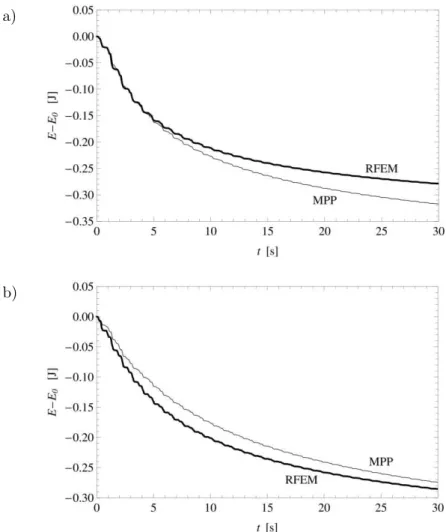
Detailed comparative studies focused on dynamics itsels are beyond the scope of this paper. However, to illustrate an agreement rate of the two systems, their total energy E = T+V is shown in Fig. 5. To make the both cases fully comparable, the initial energy E0 is regarded as the zero level. In more systematic analysis the difference between energy of the systems should be minimized by more sophisticated selection of the parameters.
Fig. 4 Number of elements versus computation time in seconds
5 CONCLUSIONS
selec-tion of the parameters values has led to quite compatible soluselec-tions. What is more, the obtained results prove that the RFEM approach is numerically more efficient.
All in all, the RFEM is a well-developed and effective approach, which is based on simple con-ceptions and can be used to analyze both small and large deformations. The presented, numerical-ly efficient model will be useful in further, comparative studies of the rope dynamics.
a)
b)
Fig. 5 Total energy of the two systems: a n = 30, b n = 70
Acknowledgements
The paper has been presented during 11th Conference on Dynamical Systems – Theory and Applications. This work was supported by 21-381/2011 DS grant.
References
1. Fritzkowski P., Kaminski H., Dynamics of a rope as a rigid multibody system. Journal of Mechanics of Materi-als and Structures, 3(6), 2008, 1059-1075.
3. Fritzkowski P., Kaminski H., A discrete model of a rope with bending stiffness or viscous damping. Acta Mechanica Sinica, 27(1), 2011, 108-113.
4. Kruszewski J., Sawiak S., Wittbrodt E., The Rigid Finit Element Method in Dynamics of Structures. Warsaw, WNT, 1999 [in Polish].
5. Wittbrodt E., Adamiec-Wojcik I., Wojciech S., Dynamics of Flexible Multibody Systems: Rigid Finite Element Method. Berlin, Heidelberg, Springer-Verlag, 2006.
6. McLachlan N. W., Bessel Functions for Engineers. Oxford, England, Clarendon Press, 1961.
7. Gatti C., Perkins N., Physical and numerical modeling of the dynamic behavior of a y line. Journal of Sound and Vibration, 255(3), 2002, 555-577.
8. Goriely A., McMillen T., Shape of a cracking whip. Physical Review Letters, 88(24), 2002, #244301.
9. Goyal S., Perkins N.C., Lee C.L., Nonlinear dynamics and loop formation in Kirchhoff rods with implications to the mechanics of DNA and cables. Journal of Computational Physics, 209, 2005, 371-389.
10. Yong D., Strings, chains and ropes. SIAM Review, 48(4), 2006, 771-781.
11. Wong C., Yasu K., Falling chains. Physical Review Letters, 74(6), 2006, 490-496.
12. Pieranski P., Tomaszewski W., Dynamics of ropes and chains, I: The fall of the folded chain. New Journal of Physics, 7, 2005, #45.