Lat. Am. j. solids struct. vol.10 número1

Abstract

The work is focused on the problem of vibrating beams with a variable cross-section fixed on a rotational rigid disk. The beam is loaded by a transversal time varying force orthogonal to an axis of the beam and simultaneously parallel to the disk’s plane. There are many ways of usage of the technical moveable systems com-posed of elements with the variable cross-sections. The main ap-plications are used in numerous types of turbines and pumps. The paper is a kind of introduction to the dynamic analysis of above mentioned beam systems. The equations of motion of rotational beams fixed on the rigid disks were derived. After introducing the Coriolis forces and the centrifugal forces, the transportation effect in the mathematical model was considered. This particular project is the first stage research, where there were proposed certain solu-tions of problems connected with the linear variable cross-secsolu-tions systems. The further investigation considering the nonlinear sys-tems has been proceeding. The results, analysis and comparison will be presented in the future works.

Keywords

variable cross-section, beam, rotary motion, dynamic flexibility

Vibrations of beams with a variable cross-section fixed on

rotational rigid disks

1 INTRODUCTION

The fundamental elements of the numerous mechanisms or machines, namely the beams and rods, are most commonly considered as the vibrating stationary systems. In these cases they are treated as the immovable ones without the coupling between the local oscillations and the main operational motion. The mechanical systems are predominantly considered both in the kinematical and dynam-ical aspects. The main problems resulting from the analysis are connected with the issues of control-ling and stabilizing mechanical systems as such. Numerous research can be found in the literature [1, 3, 4, 7, 9, 14-16, 18-22] and so far the solutions have been found by considering the transporta-tion (considered as the main working motransporta-tion) and the local oscillatransporta-tions separately [2, 3, 5, 6, 8, 10-12, 17]. Mesut Simsek in his paper [14] presents the nonlinear dynamic analysis of a functionally graded beam with pinned-pinned supports. Simsek uses the Timoshenko beam theory with the von Karman's nonlinear strain-displacement relationships. The beam was analyzed in relation to its

Slawom ir Zolkiewski*

Silesian University of Technology, Institute of Engi-neering Processes Automation and Integrated Manu-facturing Systems, Division of Mechatronics and Designing of Technical Systems, Faculty of Mechani-cal Engineering, 18a Konarskiego Street, 44-100 Gliwice, Poland

variable thickness of a cross-section according to the power-law formula. The system of equations of motion is derived by using the Lagrange’s equations. Transverse and axial deflections and rotation of the cross-sections of the beam were expressed in polynomial forms. The boundary conditions are taken into account by using the Lagrange multipliers. The Newmark-b method in conjunction with the direct iteration method was used to solve nonlinear equations of motion. In the work, large de-flection, velocity of the moving load and excitation frequency on the beam displacements were ana-lyzed. Some detailed cases were compared with each other. Another method of analysis of high-speed rotating beams is presented in [9] by Gunda. The author introduces a new finite element for free vibration analysis of rotating beams. The basis shape functions which apply a linear combina-tion of the solucombina-tion of the governing static differential equacombina-tion of a stiff-string and a cubic polyno-mial are used. The introduced functions depend on the angular velocity and position of the analyzed section, what accounts for the centrifugal stiffening effect. In paper [1] the effects of rotary inertia were presented. The author shows the rotation impact on the extensional tensile force and the ei-genvalues of beams. The analyzed beam was rotated uniformly about a transverse axis taking into account longitudinal elasticity. The perturbation technique and Galerkin's method were used. In the example of a typical helicopter rotor blade it was indicated that the extensional tensile force in-creases up to ten percent, when the rotary inertia contribution is retained in the modelling. Szefer in [15, 16] claimed that the vibrations from flexibility of elements of the mechanical composition are much smaller than a main dislocation of this composition. There is an increased range of velocities and accelerations of such a type systems. All those are caused by using more efficient drives or/and less and less weighting materials. In order to constraint power output of drives for motion of me-chanical systems, materials with the lower mass density and stiffness are used. All those things are reasons for creating the new models of designing technical beamlike systems. The variable cross-section beams are applied in many practical applications nowadays. Both the linearly and nonlinear-ly variable cross-sections are used in technical systems. These systems should be taken under con-sideration with respect to a realistic distribution of mass and flexibility. Any variations in cross-sections cannot be neglected and should be considered in the mathematical model assumptions. In spite of many works [e.g. 1, 9-12, 17, 22], where their authors analyzes the beams in rotations and beams with variable cross-sections, this work is devoted to general analyses both the linear and non-linear ones of vibrating transversally beams with the variable cross-section. It is believed that new equations and results are presented in this paper.

2 MODEL OF THE ANALYZED BEAMS FIXED ON THE ROTATIONAL RIGID DISK

 

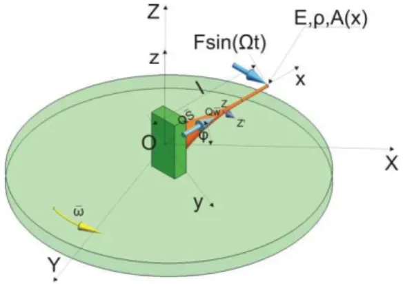
Fig. 1 Model of the analyzed beam on the rotational disk [3]

Fig. 2 Model of the analyzed beam on the rotational disk – the XZ projection [3]

where: ρ – mass-density, A(x) – cross-section, l – length of the beam, x – location of the ana-lyzed cross-section, ω – angular velocity, Ω – frequency, Q – rotation matrix, S – position vector, F – harmonic force, E – Young modulus, w – vector of displacement.

There is defined a set of generalized coordinates allowing to make an assumption that general-ized coordinates are the orthogonal projections on the coordinate axes of the global reference frame and can be written thus:

1 X,

q =r ₍₁₎

2 Y,

q =r ₍₂₎

and after differentiating (Eq. 1) and (Eq. 2) can be obtained the generalized velocities in the form:



q₁ =dq1 dt

=r

X =vX, (3)

 q₂ =

dq₂ dt

=r

or in the equivalent vector form expressing the displacements:

r =[rX,rY] T

(5)

and the equivalent vector expressing the velocities:



r =[rX,rY] T

. (6)

The cross-section is dependent on the x coordinate and for instance making an assumption that the analyzed beam is a cone (a base with radius equal x/l) it can be written as follows:

A x

( )

=A

0 1−

x

l

⎛ ⎝ ⎜⎜ ⎜

⎞ ⎠ ⎟⎟ ⎟⎟

2

=π ₁₋x

l

⎛ ⎝ ⎜⎜ ⎜

⎞ ⎠ ⎟⎟ ⎟⎟

2

, (7)

The angular velocity of the rotational disk treated as the transportation velocity is defined as:

ω= ⎡ _{0 0 ω}

⎣ ⎤⎦

T

, (8)

The location of the analyzed cross-section is described by the position vector defined as follows:

S = ⎡ s 0 0 ⎣⎢ ⎤⎦⎥

T

. (9)

The xyz reference frame is the rotational one and the matrix allowing expressing vectors is the rotation matrix. The xyz local reference frame is fixed to the rotating beam and its z-axis coincides with the rotation axis of the rigid disk, thus the rotation matrix is defined as such:

Q=

cosϕ ₋sinϕ 0 sinϕ cosϕ 0

0 0 1

⎡

⎣ ⎢ ⎢ ⎢ ⎢ ⎢

⎤

⎦ ⎥ ⎥ ⎥ ⎥ ⎥

. ₍₁₀₎

 

w

( )

0,t = 0, ∂w

( )

0,t

∂x

=0,

∂2_{w l}

( )

_,t

∂x2

= 0,

∂ ∂x

EI

( )

x ∂ w2 _l

,t

( )

∂x2

⎡

⎣ ⎢ ⎢ ⎢

⎤

⎦ ⎥ ⎥ ⎥ =−

2 F

0δ

(

x−l

)

cos

( )

Ωt dx,

0 l

∫

⎧

⎨ ⎪⎪ ⎪⎪ ⎪⎪ ⎪⎪ ⎪⎪ ⎪

⎩ ⎪⎪ ⎪⎪ ⎪⎪ ⎪⎪ ⎪⎪ ⎪

(11)

in every time moment t ≥ _0.

For the beams with the linearly variable cross-section the geometric moment of inertia can be assumed as the function proportional to the constant initial moment I0 for example as:

I

( )

x = I 0 1−

x

l

⎛ ⎝ ⎜⎜ ⎜

⎞ ⎠ ⎟⎟ ⎟⎟

4

. (12)

After solving the boundary value problem, the eigenfunction for the displacement can be derived in the form:

X x

( )

=

x

−

n

2

C

1

J

n

(

k x

)

+

C

₂

Y

n

(

k x

)

+

C

3

I

n

(

k x

)

+

C

₄

K

n

(

k x

)

⎡

⎣⎢ ⎤⎦⎥

,

(13)

where [13]:

Jn – the Bessel function of the first kind, Yn – the Bessel function of the second kind, In – the hyperbolic Bessel function of the first kind, Kn – the hyperbolic Bessel function of the second kind,

C1,2,3,4 – the integrations constants, where: n is a mode of vibrations of the beam with a variable

cross-section. The k coefficient is a linear approximation of the realistic eigenvalues of the analyzed systems.

3 EQUATIONS OF MOTION OF THE ANALYZED SYSTEMS

ρA x

( )

cosϕ −sinϕ 0

sin_ϕ cosϕ 0

0 0 1

⎡ ⎣ ⎢ ⎢ ⎢ ⎢ ⎢ ⎤ ⎦ ⎥ ⎥ ⎥ ⎥ ⎥ 0 0

∂2_w

∂t2 ⎡ ⎣ ⎢ ⎢ ⎢ ⎢ ⎢ ⎢ ⎢ ⎢ ⎤ ⎦ ⎥ ⎥ ⎥ ⎥ ⎥ ⎥ ⎥ ⎥

−_ρA x

( )

cosϕ −sinϕ 0

sin_ϕ cosϕ 0

0 0 1

⎡ ⎣ ⎢ ⎢ ⎢ ⎢ ⎢ ⎤ ⎦ ⎥ ⎥ ⎥ ⎥ ⎥

ω2s

0 0 ⎡ ⎣ ⎢ ⎢ ⎢ ⎢ ⎢ ⎤ ⎦ ⎥ ⎥ ⎥ ⎥ ⎥ +

+ρA x

( )

cosϕ −sinϕ 0

sin_ϕ cosϕ 0

0 0 1

⎡ ⎣ ⎢ ⎢ ⎢ ⎢ ⎢ ⎤ ⎦ ⎥ ⎥ ⎥ ⎥ ⎥ 0  ωs 0 ⎡ ⎣ ⎢ ⎢ ⎢ ⎢ ⎢ ⎤ ⎦ ⎥ ⎥ ⎥ ⎥ ⎥

=−EI x

( )

cosϕ −sinϕ 0 sin_ϕ cosϕ 0

0 0 1

⎡ ⎣ ⎢ ⎢ ⎢ ⎢ ⎢ ⎤ ⎦ ⎥ ⎥ ⎥ ⎥ ⎥ 0 0

∂4_w

∂x4

⎡ ⎣ ⎢ ⎢ ⎢ ⎢ ⎢ ⎢ ⎢ ⎢ ⎤ ⎦ ⎥ ⎥ ⎥ ⎥ ⎥ ⎥ ⎥ ⎥ + −2∂

EI x

( )

∂x

cosϕ −sinϕ 0

sin_ϕ cosϕ 0

0 0 1

⎡ ⎣ ⎢ ⎢ ⎢ ⎢ ⎢ ⎤ ⎦ ⎥ ⎥ ⎥ ⎥ ⎥ 0 0

∂3_w

∂x3 ⎡ ⎣ ⎢ ⎢ ⎢ ⎢ ⎢ ⎢ ⎢ ⎢ ⎤ ⎦ ⎥ ⎥ ⎥ ⎥ ⎥ ⎥ ⎥ ⎥ −∂ 2_{EI x}

( )

∂x2

cos_ϕ −sin_ϕ 0

sin_ϕ cosϕ 0

0 0 1

⎡ ⎣ ⎢ ⎢ ⎢ ⎢ ⎢ ⎤ ⎦ ⎥ ⎥ ⎥ ⎥ ⎥ 0 0 ∂2_w

∂x2 ⎡ ⎣ ⎢ ⎢ ⎢ ⎢ ⎢ ⎢ ⎢ ⎢ ⎤ ⎦ ⎥ ⎥ ⎥ ⎥ ⎥ ⎥ ⎥ ⎥ (14)

in each point of the range D =

{

(

x_,t

)

_,x ∈

( )

0,l _,t >0

}

the Eq. (3.1) coincides with boundary con-ditions and initials concon-ditions.

The projections of the equations of motion in the global reference frame are obtained from the Eq. (14) and in the XYZ global reference frame equations for individual axes can be expressed as:

ω2scosϕ+ωssinϕ =0, (15)

ω2ssinϕ−ωs cosϕ =0, (16)

ρA x

( )

∂ 2_w

∂t2

+EI

( )

x ∂ 4_w

∂x4

+₂

∂EI

( )

x

∂x

∂3w ∂x3

+

∂2_{EI x}

( )

∂x2 ∂2w ∂x2

=0. ₍₁₇₎

Third governing equation (17) is a well-known one and represents the equation of motion of the immovable beam with the variable cross-section.

 

Fig. 3 Model of the analyzed beam with the linearly variable cross-section fixed on the rotational disk and loaded by a transversal force orthogonal to an axis of the beam and parallel to the disk’s plane [3]

Analogically to the previous equations of motion it can be derived by means of the classical method. Interesting case of the loading is the beam loaded by a transversal time varying force or-thogonal to an axis of the beam and simultaneously parallel to the disk’s plane. The obtained equa-tions of motion are coupled ones with the Coriolis elements. After loading the beam in the direction of the y axis of the local reference frame it can be derived the equations of motion of the beam in the matrix form. This system of equations of motion is the fourth order partial differential equations (PDE) and can be expressed as follows:

ρA x

( )

cos_{ϕ −}sin_ϕ 0 sinϕ cosϕ 0

0 0 1

⎡ ⎣ ⎢ ⎢ ⎢ ⎢ ⎢ ⎤ ⎦ ⎥ ⎥ ⎥ ⎥ ⎥ 0

∂2_w ∂t2 0 ⎡ ⎣ ⎢ ⎢ ⎢ ⎢ ⎢ ⎢ ⎤ ⎦ ⎥ ⎥ ⎥ ⎥ ⎥ ⎥

−ρA x

( )

cos_{ϕ −}sin_ϕ 0 sinϕ cosϕ 0

0 0 1

⎡ ⎣ ⎢ ⎢ ⎢ ⎢ ⎢ ⎤ ⎦ ⎥ ⎥ ⎥ ⎥ ⎥

ω2s ω2w

0 ⎡ ⎣ ⎢ ⎢ ⎢ ⎢ ⎤ ⎦ ⎥ ⎥ ⎥ ⎥ +

−2ρA x

( )

cosϕ −sinϕ 0 sinϕ cosϕ 0

0 0 1

⎡ ⎣ ⎢ ⎢ ⎢ ⎢ ⎢ ⎤ ⎦ ⎥ ⎥ ⎥ ⎥ ⎥

ω∂w

∂t 0 0 ⎡ ⎣ ⎢ ⎢ ⎢ ⎢ ⎢ ⎢ ⎢ ⎢ ⎤ ⎦ ⎥ ⎥ ⎥ ⎥ ⎥ ⎥ ⎥ ⎥

+ρA x

( )

cosϕ −sinϕ 0 sinϕ cosϕ 0

0 0 1

⎡ ⎣ ⎢ ⎢ ⎢ ⎢ ⎢ ⎤ ⎦ ⎥ ⎥ ⎥ ⎥ ⎥

−_ωw  ωs 0 ⎡ ⎣ ⎢ ⎢ ⎢ ⎢ ⎤ ⎦ ⎥ ⎥ ⎥ ⎥ = =−

cos_{ϕ −}sin_ϕ 0 sinϕ cosϕ 0

0 0 1

⎡ ⎣ ⎢ ⎢ ⎢ ⎢ ⎢ ⎤ ⎦ ⎥ ⎥ ⎥ ⎥ ⎥ 0 ∂2 ∂x2

EI

( )

x ∂ 2w

∂x2

⎛ ⎝ ⎜⎜ ⎜⎜ ⎞ ⎠ ⎟⎟ ⎟⎟ 0 ⎡ ⎣ ⎢ ⎢ ⎢ ⎢ ⎢ ⎢ ⎤ ⎦ ⎥ ⎥ ⎥ ⎥ ⎥ ⎥ (18)

in each point of the range D ₌

_{

₍

x t,

₎

,x Œ

_{( )}

0,l ,t _>0

_}

the Eq. (18) coincides with boundary

condi-tions and initials condicondi-tions.

The projection onto the X and Y axes, can be obtained, where the projection onto the X axis of the global reference frame is as follows:

ρA x

( )

∂

2_w X ∂t2

+ ∂

2 ∂x2

EI

( )

x ∂ 2_w

X

∂x2 ⎛ ⎝ ⎜⎜ ⎜⎜ ⎞ ⎠ ⎟⎟

⎟⎟⎟−2ρA x

( )

ω∂ w

Y ∂t

+

−ρA x

( )

ωw

Y +ωs sinϕ

(

)

=ρA x

( )

ω2 w

X +scosϕ

(

)

,

and for the Y axis of the global reference frame, the projection can be written:

ρA x

( )

∂ 2_w

Y ∂t2

+ ∂

2 ∂x2

EI

( )

x ∂

2_w

Y

∂x2 ⎛

⎝ ⎜⎜ ⎜⎜

⎞

⎠ ⎟⎟

⎟⎟⎟+2ρA x

( )

ω∂ w

X

∂t

+

+ρA x

( )

ωw

X +ωs cosϕ

(

)

=ρA x

( )

ω2 w

Y +ssinϕ

(

)

,

(20)

where using the real coordinates the individual displacements onto the axes of the global reference frame are:

w

X =−wsinϕ, w

Y =wcosϕ.

(21)

It is obvious that the vibrating beams can be described by different boundary conditions for different loading and fixations types and this case can be treated as the general one.

4 MATHEMATICAL MODEL OF THE SYSTEM

The mathematical model of the analyzed beam is provided by the orthogonalization of the equa-tions of motion (19) and (20). The orthogonalization is provided by the Eqs. (19) and (20) which are multiplied using the eigenfunction for the displacements and computing integrals from the equa-tions of motion in the beams limits of integration from the origin of the beam (zero) to the end (a length of the beam). After assuming a constant angular velocity, an angular acceleration equals zero and after introducing Eqs. (21), then the projecting equations of motion Eq. (18) onto the axes of the global reference frame can be written:

ρA x

( )

∂ 2_w

X

∂t2

X x

( )

dx 0

l

∫

+ EI x

( )

∂

4_w

X

∂x4

X x

( )

dx 0

l

∫

+

+₂ ∂ EI

( )

x

∂x

∂3_w

X

∂x3

X x

( )

dx + 0

l

∫

∂2EI_∂

( )

x

x2

∂2w X

∂x2

X x

( )

dx + 0

l

∫

−₂ρ A x

( )

_ω∂wY ∂t

X x

( )

dx

0 l

∫

− ρA x

( )

_ω2_w

XX x

( )

dx

0

l

∫

=0,

(22)

and for the second equation, also multiplied by the eigenfunction for displacement and integrated along the beam:

ρA x

( )

∂

2_w

Y

∂t2

X x

( )

dx 0

l

∫

+ EI x

( )

∂

4_w Y ∂x4

X x

( )

dx

0

l

∫

+

+₂ ∂ EI

( )

x

∂x

∂3_w Y

∂x3

X x

( )

dx + 0

l

∫

∂2EI_∂

( )

x

x2

∂2_w

Y ∂x2

X x

( )

dx+

0

l

∫

+₂ρ A x

( )

_ω∂wX

∂t

X x

( )

dx

0

l

∫

− ρA x

( )

_ω2_w

YX x

( )

dx

0 l

∫

= 0.

 

The presented mathematical model is universal for different functions describing the variability of the beam’s cross-section. The cross-section of the analyzed beam can be now treated as both line-arly and nonlineline-arly variable. If the beam has the nonlineline-arly variable cross-section (Fig. 4-5) the appropriate function describing this variation ought to be adopted. The different loading terms can be considered as well. For example the beam is loaded by a transversal force orthogonal to an axis of the beam and orthogonal to the disk’s plane (Fig. 4) or the beam is loaded by a transversal force orthogonal to an axis of the beam and in parallel to the disk’s plane (Fig. 5).

Fig. 4 Model of the analyzed beam with the nonlinearly variable cross-section fixed on the rotational disk and loaded by a transversal force orthogonal to an axis of the beam and orthogonal to the disk’s plane

These cases can be considered separately or combined. According to the scientific literature the case presented in figure 4 is well-known in the mathematical sense, likewise the case in figure 1.

Fig. 5 Model of the analyzed beam with the nonlinearly variable cross-section fixed on the rotational disk and loaded by a transversal force orthogonal to an axis of the beam and in parallel to the plane of the disk

E X x

( )

I

( )

x ∂ 3_w

X

∂x3

−∂X x

( )

I

( )

x ∂x

∂2_w X ∂x2

+∂

2_{X x}

_{( )}

_I

_{( )}

_x ∂x2

∂w X

∂x

⎡

⎣ ⎢ ⎢ ⎢

⎤

⎦ ⎥ ⎥ ⎥ 0 l

+

−E∂

3_{X x}

( )

I

( )

x

∂x3

w X

0

l

+E I x

( )

XIV

( )

x w

Xdx 0

l

∫

+

+₄E I′

( )

x X′′′

( )

x w Xdx

0 l

∫

+6E I′′

( )

x X′′

( )

x w Xdx

0 l

∫

+

+₄E I′′′

( )

x X′

( )

x w Xdx +

0 l

∫

E IIV

( )

x X x

( )

w

Xdx+ 0

l

∫

+ ρA x

( )

∂ 2w

X

∂t2

X x

( )

dx

0

l

∫

+

+₂E X x

( )

I′

( )

x ∂ 2_w

X ∂x2 −

∂X x

( )

I′

( )

x

∂x

∂w

X

∂x +

∂2_{X x}

_{( )}

_I′

_{( )}

_x ∂x2

w

X

⎡

⎣ ⎢ ⎢ ⎢

⎤

⎦ ⎥ ⎥ ⎥

0

l

+

−₂E I′

( )

x X′′′

( )

x w Xdx −

0

l

∫

6E I′′

( )

x X′′

( )

x w Xdx +

0

l

∫

−6E I′′′

( )

x X′

( )

x w

Xdx

0

l

∫

−₂E IIV

( )

x X x

( )

w

Xdx

0

l

∫

+

+E X x

( )

I′′

( )

x ∂wX

∂x −

∂X x

( )

I′′

( )

x ∂x

w

X

⎡

⎣ ⎢ ⎢ ⎢

⎤

⎦ ⎥ ⎥ ⎥₀

l

+E I′′

( )

x X′′

( )

x w

Xdx + 0

l

∫

+₂E I′′′

( )

x X′

( )

x w

Xdx +E I IV _x

( )

X x

( )

w Xdx+

0 l

∫

0

l

∫

−₂ρ A x

( )

_ω∂wY

∂t

X x

( )

dx

0

l

∫

− ρA x

( )

_ω2w

XX x

( )

dx 0

l

∫

=0,

(24)

 

E X x

( )

I

( )

x ∂ 3_w

Y

∂x3

−∂X x

( )

I

( )

x ∂x

∂2_w

Y

∂x2

+∂

2_{X x}

_{( )}

_I

_{( )}

_x

∂x2

∂w Y

∂x

⎡

⎣ ⎢ ⎢ ⎢

⎤

⎦ ⎥ ⎥ ⎥ 0 l

+

−E∂ 3_{X x}

( )

I

( )

x

∂x3

w

Y

0

l

+E I x

( )

XIV

( )

x w

Ydx

0

l

∫

+

+₄E I′

( )

x X′′′

( )

x w Ydx 0

l

∫

+6E I′′

( )

x X′′

( )

x w Ydx 0

l

∫

+

+₄E I′′′

( )

x X′

( )

x w Ydx +

0

l

∫

E IIV

( )

x X x

( )

w

Ydx+ 0

l

∫

+ ρA x

( )

∂

2w Y ∂t2

X x

( )

dx

0

l

∫

+

+₂E X x

( )

I′

( )

x ∂ 2_w

Y

∂x2

−∂X x

( )

I′

( )

x ∂x

∂w

Y

∂x +

∂2_{X x}

_{( )}

_I′

_{( )}

_x ∂x2

w Y ⎡

⎣ ⎢ ⎢ ⎢

⎤

⎦ ⎥ ⎥ ⎥ 0 l

+

−₂E I′

( )

x X′′′

( )

x w

Ydx− 0

l

∫

6E I′′

( )

x X′′

( )

x w

Ydx 0

l

∫

+

−6E I′′′

( )

x X′

( )

x w Ydx 0

l

∫

−₂E IIV

( )

x X x

( )

w

Ydx 0

l

∫

+

+E X x

( )

I′′

( )

x ∂wY ∂x −

∂X x

( )

I′′

( )

x

∂x w

Y ⎡

⎣ ⎢ ⎢ ⎢

⎤

⎦ ⎥ ⎥ ⎥₀

l

+E I′′

( )

x X′′

( )

x w Ydx+ 0

l

∫

+₂E I′′′

( )

x X′

( )

x w

Ydx+E I IV _x

( )

X x

( )

w

Ydx + 0

l

∫

0

l

∫

+₂ρ A x

( )

_ω∂wX ∂t

X x

( )

dx

0 l

∫

− ρA x

( )

_ω2w

YX x

( )

dx 0

l

∫

=0.

(25)

E X x

( )

I

( )

x ∂ 3_w

X

∂x3 −

∂X x

( )

I

( )

x ∂x

∂2_w

X ∂x2

+∂

2_{X x}

_{( )}

_I

_{( )}

_x

∂x2

∂w X ∂x ⎡ ⎣ ⎢ ⎢ ⎢ ⎤ ⎦ ⎥ ⎥ ⎥ 0 l +

−E∂

3_{X x}

( )

I

( )

x ∂x3

w

X

0

l

+E I x

( )

XIV

( )

x w Xdx

0 l

∫

+₂E I′

( )

x X′′′

( )

x w

Xdx 0

l

∫

+

+ ρA x

( )

∂

2w X

∂t2

X x

( )

dx

0 l

∫

+E I′′

( )

x X′′

( )

x w

Xdx +

0

l

∫

+₂E X x

( )

I′

( )

x ∂

2_w X ∂x2

−∂X x

( )

I′

( )

x ∂x

∂w X

∂x +

∂2_{X x}

_{( )}

_I′

_{( )}

_x

∂x2 w X ⎡ ⎣ ⎢ ⎢ ⎢ ⎤ ⎦ ⎥ ⎥ ⎥₀ l +

+E X x

( )

I′′

( )

x ∂wX

∂x −

∂X x

( )

I′′

( )

x ∂x w X ⎡ ⎣ ⎢ ⎢ ⎢ ⎤ ⎦ ⎥ ⎥ ⎥0 l +

−2ρ A x

( )

_ω∂wY

∂t

X x

( )

dx

0

l

∫

− ρA x

( )

_ω2w

XX x

( )

dx 0

l

∫

= 0,

(26)

and the coupled second equation:

E X x

( )

I

( )

x ∂

3_w

Y

∂x3 −

∂X x

( )

I

( )

x

∂x

∂2_w

Y ∂x2 +

∂2_{X x}

_{( )}

_I

_{( )}

_x

∂x2

∂w Y ∂x ⎡ ⎣ ⎢ ⎢ ⎢ ⎤ ⎦ ⎥ ⎥ ⎥₀ l +

−E∂

3_{X x}

( )

I

( )

x

∂x3 w

Y

0 l

+E I x

( )

XIV

( )

x w Ydx 0

l

∫

+₂E I′

( )

x X′′′

( )

x w

Ydx 0

l

∫

+

+E I′′

( )

x X′′

( )

x w Ydx 0

l

∫

+ ρA x

( )

∂ 2_w

Y ∂t2

X x

( )

dx

0 l

∫

+

+₂E X x

( )

I′

( )

x ∂ 2w

Y ∂x2

−∂X x

( )

I′

( )

x ∂x

∂w Y ∂x +

∂2_{X x}

_{( )}

_I′

_{( )}

_x

∂x2 w Y ⎡ ⎣ ⎢ ⎢ ⎢ ⎤ ⎦ ⎥ ⎥ ⎥₀ l +

+E X x

( )

I′′

( )

x ∂wY ∂x −

∂X x

( )

I′′

( )

x

∂x w Y ⎡ ⎣ ⎢ ⎢ ⎢ ⎤ ⎦ ⎥ ⎥ ⎥0 l

+₂ρ A x

( )

_ω∂wX

∂t

X x

( )

dx +

0 l

∫

− ρA x

( )

_ω2w

YX x

( )

dx 0

l

∫

=0.

(27)

There are introduced the equivalent notation for the eigenfunctions, cross-sections and the mo-ments of inertia as:

 

The Eqs. (26) and (27) after substituting (28) are simplified to:

E XI∂

3_w

X ∂x3 −

′

X I +XI′

(

)

∂2wX

∂x2

+

(

X I′′ +₂X′I′+XI′′

)

∂wX ∂x ⎡ ⎣ ⎢ ⎢ ⎢ ⎤ ⎦ ⎥ ⎥ ⎥0 l +

−E

(

X I′′′ +3X′′I′+3X′I′′+I X′′′

)

w X ₀

l

+E IXIVw Ydx

0 l

∫

+

+2E I′X w′′′ Xdx

0 l

∫

+E I′′X w′′ Xdx

0 l

∫

+ ρA∂

2_w X ∂t2

X dx

0 l

∫

+

+E 2XI′∂ 2

w_X

∂x2 −

2

(

X′I′+XI′′

)

∂wX

∂x +2 ′′

X I′+₂X′I′′+I X′′′

(

)

w

X ⎡ ⎣ ⎢ ⎢ ⎢ ⎤ ⎦ ⎥ ⎥ ⎥0 l +

+E XI′′∂wX

∂x − ′

XI′′+XI′′′

(

)

w

X ⎡ ⎣ ⎢ ⎢ ⎤ ⎦ ⎥ ⎥ 0 l

−2_ρ A_ω∂wY ∂t

X dx

0

l

∫

− ρA_ω2_w

XX dx

0 l

∫

=0

(29)

and analogically to the second equation (27) for the Y axis of the global reference frame can be ob-tained as:

E XI∂ 3

w_Y

∂x3 −

(

X I′ +XI′

)

∂2_w

Y

∂x2 +

(

X I′′ +2X′I′+XI′′

)

∂w_Y

∂x ⎡ ⎣ ⎢ ⎢ ⎢ ⎤ ⎦ ⎥ ⎥ ⎥0 l +

−E

(

X I′′′ +3X′′I′+3X′I′′+I X′′′

)

w

Y ₀ l

+E IXIVw

Ydx

0

l

∫

+

+2E I′X w′′′ _Ydx

0

l

∫

+E I′′X w′′ _Ydx 0

l

∫

+ ρA∂

2

w_Y

∂t2

X dx

0 l

∫

+

+E 2XI′∂

2

w

Y

∂x2 −

2

(

X′I′+XI′′

)

∂wY

∂x +2

(

X′′I′+2X′I′′+I X′′′

)

wY

⎡ ⎣ ⎢ ⎢ ⎢ ⎤ ⎦ ⎥ ⎥ ⎥0 l +

+E XI′′∂wY

∂x −

(

X′I′′+XI′′′

)

wY

⎡ ⎣ ⎢ ⎢ ⎤ ⎦ ⎥ ⎥ 0 l

+2_ρ A_ω∂wX

∂t X dx

0 l

∫

− ρA_ω2w_YX dx

0 l

∫

=0.

(30)

E XI∂ 3_w

X ∂x3 − ′

X I−XI′

(

)

∂2wX

∂x2 + ′′ X I∂wX

∂x ⎡

⎣ ⎢ ⎢ ⎢

⎤

⎦ ⎥ ⎥ ⎥₀

l

+

−E

(

X I′′′ +X′′I′

)

w X ₀

l

+E IXIVw Xdx +

0 l

∫

+2E I′X w′′′ Xdx

0 l

∫

+E I′′X w′′ Xdx

0 l

∫

+ ρA∂

2_w X ∂t2

X dx +

0 l

∫

−2ρ Aω∂ w

Y

∂t X dx

0

l

∫

− ρAω2w

XX dx

0 l

∫

=0,

(31)

the second equation (30) additionally after simplifying the integrals:

E XI∂

3_w

Y ∂x3

−

(

X I′ −XI′

)

∂

2_w

Y ∂x2

+X I′′ ∂wY ∂x ⎡

⎣ ⎢ ⎢ ⎢

⎤

⎦ ⎥ ⎥ ⎥0

l

+

−E

(

X I′′′ +X′′I′

)

w Y ₀

l

+E ∂

2_IX′′

∂x2 w

Ydx

0

l

∫

+ ρA∂

2_w

Y ∂t2

X dx

0

l

∫

+

+2_{ρ A}ω∂wX ∂t

X dx

0

l

∫

− ρAω2w

YX dx 0

l

∫

=0.

(32)

By introducing the acting external force, it can be noticed:

EI∂ 3_w

X

( )

l ∂x3

−EI′∂

2_w

X

( )

l ∂x2

=_0,

EI∂

3_w

Y

( )

l

∂x3

−EI′∂ 2_w

Y

( )

l

∂x2

=−2 F

0δ

(

x−l

)

cos

( )

Ωt dx

0

l

∫

.

(33)

Based on the boundary conditions (11) it can be written:

∂2_w X

( )

l

∂x2 = ∂2_w

Y

( )

l ∂x2 =0,

XI ∂3w

X

( )

0

∂x3

−∂XI ∂x

∂2w X

( )

0

∂x2

=_0,

XI ∂3w

Y

( )

0

∂x3

−∂XI ∂x

∂2w

Y

( )

0

∂x2

= ₀

  and

E X I′′ ∂wX

∂x −

∂X I′′

∂x wX

⎡

⎣ ⎢ ⎢

⎤

⎦ ⎥ ⎥

0

l

=_0,

E X I′′ ∂wY ∂x

−∂X I′′

∂x w

Y ⎡

⎣ ⎢ ⎢

⎤

⎦ ⎥ ⎥

0

l

=0.

(35)

By introducing (34-35) the first equation yields:

E IXIVw

Xdx +

0 l

∫

2E I′X w′′′

Xdx

0 l

∫

+E I′′X w′′

Xdx

0 l

∫

+ ρA∂

2_w X

∂t2

X dx +

0 l

∫

−2_{ρ A}ω∂ w

Y

∂t X dx

0 l

∫

− ρAω2w

XX dx 0

l

∫

= 0.

(36)

Where the searched solutions are defined as displacements in the global reference frame and the ones are separable in time and space domains. The system is symmetric and the motion of the ana-lyzed cross-section is given by the multiplication of the projected harmonic time dependent eigen-functions with the frequency Ω and the eigenfunctions for displacements with amplitudes XY. Both the variables coincide with the responses of two decoupled harmonic oscillators. In the present case the searched solutions are:

w

X = aXX x

( )

sin

( )

Ωt , n=1

∞

∑

w

Y = aYX x

( )

cos

( )

Ωt . n=₁

∞

∑

(37)

The norm for Eqs. (36) is assumed as:

γn

2 _{= AX}2_dx

0 l

∫

, (38)

I1= 1

γn

2 IX

2_dx

0 l

∫

,

I

2 =

1

γn 2

′′

I X2dx

0 l

∫

,

c = E ρ.

(39)

It can be also noticed that:

′′′ X I′

0 l

∫

dx =0. ₍₄₀₎

The a coefficients (amplitudes) can be obtained as:

a

X =

−2ω_ΩF 0X l

( )

ργn2 c4k4

(

I₂−I₁k2

)

2

+

(

ω2_{− Ω}2

)

2+₂c2k2 I

2−I1k2

(

)

(

ω2+_Ω2

)

⎡ ⎣ ⎢ ⎢

⎤ ⎦ ⎥ ⎥ ,

(41)

a

Y =

F 0X l

( )

2ργn

2

−1

I

2k 2_−c2_I

1k

4₊

(

_ω2_{− Ω}2

)

2

− 1

I 2k

2_−c2_I 1k

4₊

(

_ω2_+Ω2

)

2

⎧ ⎨ ⎪⎪ ⎪⎪

⎩ ⎪⎪ ⎪⎪

⎫ ⎬ ⎪⎪ ⎪⎪

⎭ ⎪⎪ ⎪⎪

. (42)

Knowing these amplitudes the total displacements can be calculated and the solution in the global reference frame can be obtained.

5 DYNAMICAL FLEXIBILITIES

According to the author the dynamical flexibility is understood as the amplitude of generalized dis-placement in the direction of “i” generalized coordinate changed by generalized harmonic force with amplitude equals 1 in the direction of “k” generalized coordinate. This definition can be written in the mathematical form as:

1si =Yik ₂sk. (43)

Finally the dynamical flexibility of the rotating beam with the variable cross-section is presented as:

Y = 1

2ργn2

−X x

( )

X l

( )

I 2k

2_−c2_I

1k

4₊

(

_ω2_{− Ω}2

)

2

− X x

( )

X l

( )

I

2k 2_−c2_I

1k

4₊

(

_ω2_+Ω2

)

2 ⎧

⎨ ⎪ ⎪ ⎪ ⎪

⎩ ⎪ ⎪ ⎪ ⎪

⎫

⎬ ⎪ ⎪ ⎪ ⎪

⎭ ⎪ ⎪ ⎪ ⎪ n=₁

∞

 

For comparison, the dynamical flexibility of the rotating beam with a constant cross-section is as follows:

Y_g =

X x

( )

X l

( )

(

c_g2_k4_−ω2_{− Ω}2

)

ρA_constγ_gn2 c_g4

k8

+

(

ω2− Ω2

)

2_−2c

g2k4

(

ω2 +Ω2

)

⎡

⎣ ⎢ ⎢

⎤

⎦ ⎥ ⎥ n=₁

∞

∑

.

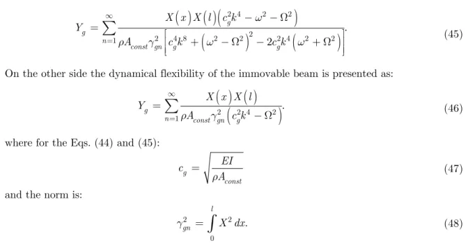
(45)

On the other side the dynamical flexibility of the immovable beam is presented as:

Y_g = X x

( )

X l

( )

ρA_constγ

gn2

(

cg2k4− Ω2

)

n=1 ∞

∑

. ₍₄₆₎

where for the Eqs. (44) and (45):

c_g = EI

ρA_const (47)

and the norm is:

γ_gn2 = _X2_dx

0 l

∫

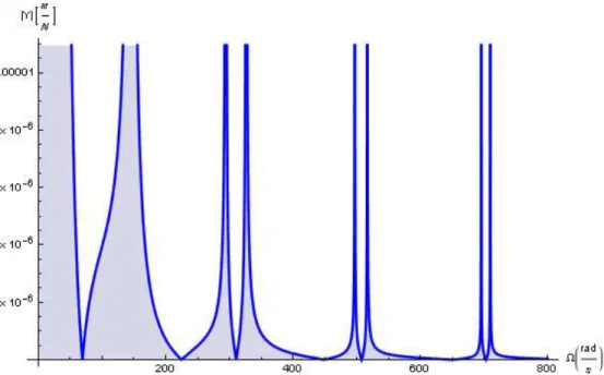
. ₍₄₈₎

Both the derived dynamical flexibilities, the Eq. (44) and Eq. (46), are presented in figures (Fig. 6-7). For numerical examples the beam of 1m length is assumed. The beam is the clamped-free one and fixed on the rotational disk. Distinctively from the beam with a constant cross-section, the beam with the variable cross-section has different inconstant bifurcations for the individual modes of vibrations (Fig. 7).

Fig. 7 Dynamical flexibility of the rotating beam with the variable cross-section. The disk is being rotated with the angular velocity equals 100 radians per second

Derivations of suitable dynamical flexibilities are applied to the systems in the transportable motion both vibrating longitudinally and transversally. The solutions can be presented on charts of amplitude (dynamical flexibility) in function of frequency. There are many numerical applications that can be used for this purpose, e.g. GENTA’S DynRot or author’s program the Modyfit [18].

Conclusions

exam- 

ples for beamlike systems with the variable cross-section will be presented and the rotating beam with damping forces considered will be analyzed. The rotating beam with some imperfections and defects or cracks can be the potential material for the further analysis and research.

Acknowledgments: the paper was presented during 11th Conference on Dynamical Systems - Theory and Applications.

References

Al-Ansary M. D.: Flexural vibrations of rotating beams considering rotary inertia. Computers and Structures, 69, 1998, 321-328.

Auciello N. M.: Comment on. A note on vibrating tapered beams. Journal of Sound and Vibration, 1995, 187-724. Bokhonsky A. I., Zolkiewski S.: Modelling and Analysis of Elastic Systems in Motion. Monograph, Gliwice, Silesian

University of Technology Press, 2011, p. 171.

Chang T.-P., Chang H.-C.: Vibration and buckling analysis of rectangular plates with nonlinear elastic end restraints against rotation. International Journal of Solids and Structures, 34, 18, June 1997, 2291-2301.

Cheung Y. K., Zhou D.: The free vibrations of tapered rectangular plates using a new set of beam functions with the Rayleigh–Ritz method. Journal of Sound and Vibration, 223, 5, 1999, 703-722.

Dyniewicz B., Bajer C. I.: New feature of the solution of a Timoshenko beam carrying the moving mass particle. Archives of Mechanics, 62, 5, 2010, 327-341.

Genta G.: Dynamics of Rotating Systems. New York, Springer, 2005.

Grossi RO, Bhat RB. A note on vibrating tapered beams. Journal of Sound and Vibration 1991, 147-174.

Gunda J. B., Gupta R. K., Gangul R.: Hybrid stiff-string–polynomial basis functions for vibration analysis of high speed rotating beams. Computers and Structures, 87, 2009, 254-265.

Kumar R., Kansal T.: Effect of rotation on Rayleigh waves in an isotropic generalized thermoelastic diffusive half-space. Archives of Mechanics, 60, 5, 2008, 421-443.

Ozturk H.: In-plane free vibration of a pre-stressed curved beam obtained from a large deflected cantilever beam. Finite Elements in Analysis and Design, 47, 2011, 229-236.

Rahman M. A., Kowser M. A., Hossain S. M. M.: Large deflection of the cantilever steel beams of uniform strength - experiment and nonlinear analysis. International Journal of Theoretical and Applied Mechanics, 1, 2006, 21-36. Solecki R., Szymkiewicz J.: The rod and surface systems. Warszawa, Arkady Budownictwo, Sztuka, Architektura,

1964 (in Polish).

Simsek M.: Non-linear vibration analysis of a functionally graded Timoshenko beam under action of a moving har-monic load. Composite Structures, 92, 2010, 2532-2546.

Szefer G.: Dynamics of elastic bodies undergoing large motions and unilateral contact. Journal of Technical Physics. XLI, 4, 2000.

Szefer G.: Dynamics of elastic bodies in terms of plane frictional motion. Journal of Theoretical and Applied Mechan-ics, 2, 39, 2001.

Zhou D.: Vibrations of point-supported rectangular plates with variable thickness using a set of static tapered beam functions. International Journal of Mechanical Sciences, 44, 2002, 149-164.

Zolkiewski S.: Numerical Application for Dynamical Analysis of Rod and Beam Systems in Transportation. Solid State Phenomena, 164, 2010, 343-348.

Zolkiewski S.: Dynamic flexibility of the supported-clamped beam in transportation. Journal of Vibroengineering. 13, 4, December 2011, 810-816.

Zolkiewski S.: Dynamical Flexibility of Complex Damped Systems Vibrating Transversally in Transportation. Solid State Phenomena, 164, 2010 339-342.

Zolkiewski S.: Damped Vibrations Problem Of Beams Fixed On The Rotational Disk. International Journal of Bifur-cation and Chaos, 21, 10, October 2011, 3033-3041.

Zone-Ching L., Don-Tsun L.: Dynamic deflection analysis of a planar robot Computers and Structures, 53, 4, 17