Abstract
The subject of the present work is the numerical verification and experimental validation of the FEM model which would enable us to analyse the vibrations of collecting electrodes. The effectiveness of electrostatic precipitators (ESP) depends on many factors. One of these factors is the efficiency of periodic cleaning of the collecting electrodes; thus the dust is removed by inducing vibrations. These vibrations are caused by the axial impact of a hammer on an anvil beam. In the course of the impact, and afterwards, the stresses due to the impact are produced in both the rapper system and in the collect-ing electrode section. The paper presents a modified finite element method which can be used in simulations and to analyse the vibra-tions of collecting electrodes. In the verification process the calcula-tion results obtained were compared with those from commercial software (Abaqus). The calculations and measured results were com-pared for validation. The comparisons were made using peak and RMS (root-mean-squared) values as well as special factors and hit rates. An acceptable compatibility of the results proves that the model can be applied in the analysis of vibrations of electrodes in design practice.
Keywords
Laminate Composite Plate, Finite Element, Higher Order Shear De-formation, Locking Phenomenon, Assumed Strain Method
Numerical verification and experimental validation of the FEM
model of collecting electrodes in a dry electrostatic precipitator
1 INTRODUCTION
Electrostatic precipitation is a commonly used method for removing fine particles from airstreams. The effectiveness of these devices depends on many factors, such as the charging of particles, trans-porting the charged particles to the collecting surfaces, precipitation of the charged particles onto the collecting surfaces, neutralising the charged particles on the collecting surfaces, removing the particles from the collecting surface to the hopper, and conveying the particles from the hopper to a disposal point [1-4]. This research is only focused on one of these phenomena, i.e. the dislodging of particles. Removing dust collected on the electrodes is achieved by bringing them to vibrate with accelerations that allow for the effective separation of dust coagulated on their surface.
Andrzej Nowak
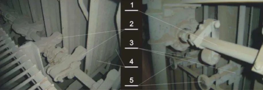
The collecting electrodes are rapped by a number of methods [5-7]. Generally, precipitator manufac-turers use hammer and anvil rappers to remove particles from the collecting electrodes. One rapper system uses hammers mounted on a rotating shaft, as shown in Figure 1. As the shaft (1) rotates, the hammers (2) drop (by gravity) and strike the anvils (5) of the anvil beams (3) that are attached to the collecting electrodes (4). The weight of the hammers and the length of their mounting arm control the rapping intensity. The frequency of the rapping can be changed by adjusting the speed of the rotating shafts. Thus, rapping intensity and frequency can be adjusted for the varying dust concentration of the flue gas.
Figure 1. Rapper system.
The next chapter presents a computational model that allowed to simulate the vibrations of collecting electrodes caused when struck during the process of shaking off dust. It has been assumed that an average class PC should be sufficient to do all of the computations, and the calculation time should not exceed several dozen minutes. Two methods were used to model the arrangement: the deformable finite element method (FEM)[8] and the rigid finite element method (RFEM)[9].
Chapter 3 presents the results of verification and validation of the model. Within the verifica-tion, and besides establishing an integration step and the density of the digitised grid of electrode plates that provide adequate precision (and convergence) of the calculation results, the results of our own calculations were compared with the results received using the Abaqus commercial pack-age. Within the process of validation, conformity of the results of our own calculations was com-pared with the results of measurements conducted on a special test stand.
2. COMPUTATIONAL MODEL
An essential feature of the finite element method is both its ability to handle complicated geome-tries (and boundaries) [8], [10] and its implementation in many commercial packages and open source software. Despite the existing commercial software, it is still necessary to search for more
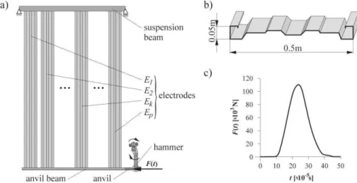
Figure 2. The most important aspects of modelling: a) schematic view of a collecting electrode system, b) SIGMA VI
profile, ) measured force impulse F(t). Vibrations are generated as the system’s response for a single force impulse F(t).
The model combines the finite element method (FEM) used to describe spring deformations [11] and mass and geometrical features of the collecting electrodes with the rigid finite element method (RFEM) [9], [12] used to reflect the behaviour of the beam segments of the modelled system. The remaining constructional elements, such as the joints that fasten the electrodes to the suspension beam, distance-marking bushes and riveted and screw joints, were considered in the model as con-centrated masses. Equations of motion of individual sub-systems (electrodes and beams) and of the
whole system were derived in the present paper from Lagrange’s equations of second order. In this
paper both geometrical and physical linear systems are taken into consideration (vibrations around the static equilibrium position). That is why it is possible to present the kinetic and potential en-ergy of deformation in quadratic forms:
1 2
T
T q Mq, (1)
T
1 2
s
V q Cq, (2)
where M C, are matrices with constant elements and q is the vector of generalised coordinates.
If the damping is passed over, then the application of Lagrange’s equation leads to the following
equations of the system’s motion:
Mq Cq G Q, (3)
where M is the mass matrix, Cis the stiffness matrix, G Vg
q , Vg is the potential energy of
of the system’s freedom. Thus, to formulate equations of the system’s (sub-system’s) motion, one should determine the mass matrixM, the stiffness matrix C, as well as vectors Gand Q.
The next sub-sections contain the basic relations that will allow to determine the matrices and vec-tors from (3) for electrodes treated as shells modelled with the deformable finite element method (FEM) [8]. A brief way will also be presented of discretising the beams modelled with the rigid fi-nite element method (RFEM), the model of joining elements which connect the beams and elec-trodes, as well as the aggregation of the sub-systems’ motion equations to equations for the whole system.
2.1 Model of shell elements
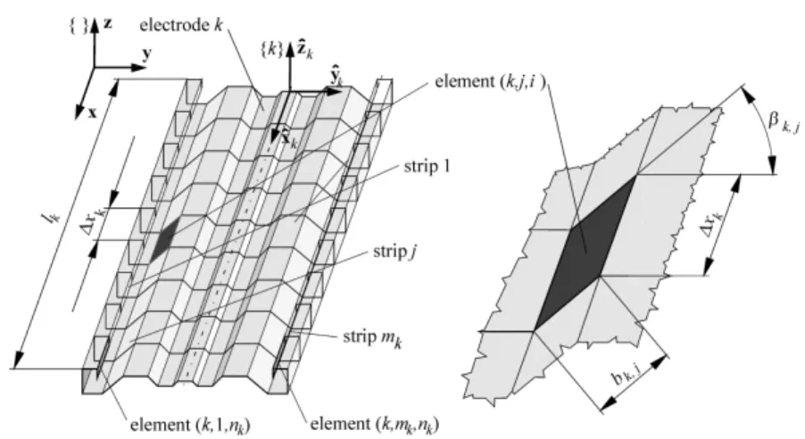
With electrode k a co-ordinate system is connected with axes directed as in Fig. 3. A single elec-trode strip has both a constant width and thickness.
This suggests how it should be divided into elements. It is assumed that the strips are numbered from 1 mk, where the first strip on the left has the number 1 while the last strip on the right has the number mk. In the ˆx direction, the strip is divided into nk elements with a length of:
k k
k
l x
n , (5)
where lk is the length of the plate (and the length of the strip is 1 mk).
Thus, the whole collecting electrode is divided into:
( )k
e k k
n m n , (6)
elements.
Figure 3. Strip j with width bk j, and inclination angle k j, towards the ˆy axis:
The strain energy of an element with the number k j i, , (Fig. 3) is independent of i (in view of the division into elements with a constant length of xk in direction ˆx) and from angle k j, . A rectangular four-node element, as presented in Fig. 4a, is considered here.
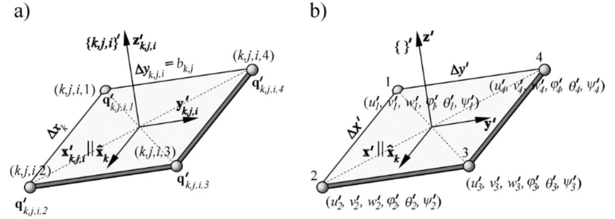
Figure 4. Four-node shell element: a) taking into consideration the following indexes: k– plate, j– strip, i– element of strip j, b) passing over indexes k, j and i.
The nodal displacements of the element are described by the following values:
T
, , , , , ,, , , ,, , , , , , , ,, , , ,, , , , for 1, 2, 3, 4 k j i s uk j i s vk j i s wk j i s k j i s k j i s k j i s s
q , (7)
where uk j i s, , , , vk j i s, , , , wk j i s, , , are displacements of node k j i s, , , in the direction of the xk j i, , ,
, , k j i
y , zk j i, , axes, respectively, and k j i s, , , , k j i s, , , , k j i s, , , are rotations in the node around the axis
parallel to xk j i, , ,yk j i, , , zk j i, , , respectively. In further considerations, during which the potential
strain energy of the element and its kinetic energy were described, indexes (k,j,i) were omitted to simplify the notation. Thus, the presented procedure refers to the element from Fig. 4b.
The nodal displacements are described by the following values:
T
, , , , , for 1, 2, 3, 4
s u v ws s s s s s s
q , (8)
It is assumed that the shield state is described by displacements u vs, s and rotation angles s ,
while displacement field u v, is described by the functions:
2 2
1 2 3 4 5 6
( , , ) u u u u u( ) u ( )
u x y t a a x a y a x y a y a x y , (9af)
2 2
1 2 3 4 5 6
( , , ) v v v v v( ) v( )
and
is described by relation [13]:1 2
u v
y x . (9c)
It is assumed that the plate state is described by deflection w and angles , , which are
described by the following relations:
( ) ( ) ( ) ( ) 2 ( ) ( ) 2
1 2 3 4 5 6
( ) 3 ( ) 2 ( ) 2 ( ) 3
7 8 9 10
( ) 3 ( ) 3
11 12
, , ( ) ( )
( ) ( ) ( ) ( )
( ) ( ) ,
w w w w w w
w w w w
w w
w x y t a a x a y a x a x y a y
a x a x y a x y a y
a x y a x y
(10a)
w
y , (10b)
w
x . (10c)
Factors ( ) ( ) ( ) ( ) 1 6 , 1 6
u u v v
a a a a and ( ) ( ) 1 12
w w
a a can be determined from the respective boundary conditions:
1 2 3
4 2, 4,
, , , , , ,
2 2 2 2 2 2
,
, , , , ,
2 2 2 2 y 2 2 y
x y x y x y
u u t u u t u u t
u
x y x y u x y
u u t u t u t
y y
(11a)
1 2 3
4 1, 3,
, , , , ,
2 2 2 2 2 2 ,
, , , , ,
2 2 2 2 x 2 2 x
x y x y x y
v v t v v v v
x y v x y v x y
v v v t v t
x x
(11b)
1 1 1
, , , , , ,
2 2 2 2 2 2
x y w x y w x y
w w t t t
y x (11c)
2 2 2
, , , , , ,
2 2 2 2 2 2
x y w x y w x y
w w t t t
y x (11d)
3 3 3
, , , , , ,
2 2 2 2 2 2
x y w x y w x y
w w t t t
4 4 4
, , , , , .
2 2 2 2 2 2
x y w x y w x y
w w t t t
y x (11f)
The strain energy of the shell element in Fig. 5b is the sum of:
( )t ( )p
E E E , (12)
where E( )t is the energy of the shield state and E( )p is the energy of the plate state. The strain
energy of the element, after necessary transformations [11], can be presented in the form of:
1,1 1,2 1,3 1,4 1
T T T T 2,1 2,2 2,3 2,4 2 1
1 2 3 4
2
3,1 3,2 3,3 3,4 3
4,1 4,2 4,3 4,4 4 4
T T
1 1
2 2
1 1 l l s
E
C C C C q
C C C C q
q q q q
C C C C q
C C C C q
q C q q
4
, , l s s C q
(13)
Where qs are specified in (8), q q1T q2T q3T q4T T and C is the square, symmetric
stiffness matrix of an element with dimensions of 24 24.
It should be noted that for the defined physical parameters of plates E, , ,h, the stiffness
matri-ces of the elements depend only on dimensions x xk and y bk j, . In view of the
designa-tion in Fig. 4 and reladesigna-tion (5), in the discussed case:
, , , , , k j i k j x bk k j
C C C , (14)
for i 1, ... , ; nk j 1, ... , mk. The formula for the strain energy of element (k,j,i) may be presented in the following form:
4 4 T 1
, , 2 , , , , , , , , , , 1 1
k j i k j i l k j i l s k j i s l s
E q C q . (15)
Thus, as a result of adopting a constant length of xk elements, the stiffness matrix of electrode
k is calculated only for j 1, ... , mk, because the stiffness matrices of elements k j i, , of the
single strip are identical.
T
T ( ) T ( ) ( ) ( ) ( )
1 1 1
2 2 2
u v p p p
T u M u v M v q M q , (16)
where ( ) ( )
,
u v
M M are matrices with dimensions of 6 x 6 while M( )p is the matrix with
dimen-sions of 12 12 with constant elements.
If the definition of vectors of nodal displacements as described in (8) is taken into consideration, then, after a proper rearrangement that runs analogically as in the case of the C stiffness matrix,
the expression for the kinetic energy of an element can be recorded in the following form:
4 4
T T
1 1
,
2 2
1 1
,
l l s s l s
T q M q q M q (17)
where Ml s, are the matrices with dimensions of 6 6 with constant elements.
As is in the case of formulae for strain energy, the expression for the kinetic energy of element
, ,
k j i may be presented in the following form:
4 4 T 1
, , 2 , , , , , , , , , , 1 1
k j i k j i l k j i l s k j i s l s
T q M q . (18)
In the computational model, the nodal displacements, expressed not in local systems but in a global co-ordinate system (5), are adopted as generalised coordinates.
Figure 5. Element k j i, , .
Let us define the following vectors:
T , , , , , , , , , , , , k j i s uk j i s vk j i s wk j i s
Δ , Δk j i s, , , uk j i s, , , vk j i s, , , wk j i s, , , T, (19a)
T , , , , , , , , , , , , k j i s k j i s k j i s k j i s
where Δk j i s, , , , Φk j i s, , , are the vectors of nodal displacements and rotations in the k j i, , sys-tem; Δk j i s, , , , Φk j i s, , , are the vectors of nodal displacements and rotations in the k j i, , system,
with axes parallel to the axis of the global system and a beginning that coincides with the
beginning of the k j i, , system. The following relations exist between them:
T , , , , , , , , , , , , , , k j i s Rk j k j i s k j i s Rk j k j i s
Δ Δ Δ Δ , (20a)
T , , , , , , , , , , , , , , k j i s Rk j k j i s k j i s Rk j k j i s
Φ Φ Φ Φ , (20b)
where , , ,
, ,
1 0 0
0 cos sin .
0 sin cos
k j k j k j
k j k j
R
Vectors qk j i s, , , and qk j i s, , , , may be presented in the following forms:
T
T T
, , , , , , , , , k j i s k j i s k j i s
q Δ Φ , (21a)
T
T T
, , , , , , , , , k j i s k j i s k j i s
q Δ Φ , (21b)
and the relations between them are described by the formulae:
, , , , , , , k j i s k j k j i s
q R q , (22a)
T , , , , , , , k j i s k j k j i s
q R q , (22b)
where , , , 0 . 0 k j k j k j R R R
Thus, formulae (18) and (15), which describe the kinetic and strain energy of element ( , , )k j i ,
may be presented in the following forms:
4 4 T
T T
1
, , 2 , , , , , , , , , , , , 1 1 4 4 T 1 , , , , , , , , , , 2 1 1
k j i k j k j i l k j i l s k j k j i s l s
k j i l k j i l s k j i s l s
T R q M R q
q M q
4 4 T T
1
, , 2 , , , , , , , , , , , 1 1
4 4 T 1
, , , , , , , , , , 2
1 1
k j i k j k j i l k j i l s k j i s l s
k j i l k j i l s k j i s l s
E R q C q
q C q
(24)
where T
, , , , , , , , , , k j i l s k j k j i l s k j
M R M R and Ck j i l s, , , , R Ck j, k j i l s, , , , RTk j, .
There are also gravity forces that influence the electrodes in the system, and they should be taken into consideration when formulating the equations of motion. Generalised forces that come from gravity forces may be presented in the following form:
( )
, , , , , , , , , for 1,2, 3, 4 u
k j i s k j i k j u s s
G N H , (25)
where
, ( ) ( )
, , , ,
k j
u u
k j i k j i
F
gh dF
N N , ( ) ( ) ( )
, ,
u u u
k j k j
N N A , ( )u 1 ( )2 ( )2
x y x y y x y
N , A( )k ju,
is a matrix with constant elements, , , , , , , ,
2 2 2 2
k j k j k j k j
k j
x x b b
F is the area of
ele-ment (k,j,i), xk j, and bk j, are described in Fig. 5, and Hk j u s, , , is a matrix with constant coeffi-cients.
2.2 Model of beam elements
When modelling the upper and lower suspension beams, the classical rigid finite element method (RFEM) was applied [9]. Fig. 6 presents the general scheme of the system. The upper beam was simply supported, while the bottom beam was rigidly connected with the electrodes and loaded with point force, as in Fig. 2c.
Figure 6. Geometric parameters of the electrode system.
There is a certain segment of beams ak assigned to each plate. The length of the beam segment is generally longer than the width of plate k. The upper and lower beams are connected to the elec-trodes with the help of e
u
assumed that nue 1and neb 2. The way of dividing the upper and lower beams into massless and non-dimensional stiffness-damping elements (sde) and rigid finite elements (rfe) is very similar. That is why the way of dividing elements into sde and rfe is presented with a general description of the beam with the symbol u b, . Fig. 7 presents the primary and secondary division of beam
.
Figure 7. Division of beams into rfe and sde: a) primary, b) secondary.
It was assumed that each of the segments a1 ap is divided into the same number of elements
s in the primary division. Moreover, segments a0 and ap 1, which are usually much shorter
than a1 ap, are not divided into smaller elements. Then, in the secondary division, the sde are
placed in the central points of the sections. The elements lying between sde are treated as rigid solids (Fig. 8).
Figure 8. Generalised coordinates of rfei: a, a, a i i i
x y z are translational displacements of the mass centre of rfe i , and
,
i i i are the rotational displacements of rfe i.
The mass parameters and coordinates of the mass centres, and thereby coordinates of sde, change when additional bodies (reinforcements, cross-bars, bushes, anvil, etc.) are added to the rfe
of the upper or lower beams. In a computer implementation of the models presented here, it was assumed that the added bodies may be represented by concentrated masses. An equation of motion for the free beam may be presented in the following form:
where q q1T qi T qnT T and qi xi yi zi i i i T is a vector of the
generalised coordinates rfe i, as in Fig. 8, M are the diagonal mass matrices with constant
coeffi-cients, C are the stiffness matrices with constant coefficients, G is the vector of gravity forces
and Q is the vector of external generalised forces. It is worth mentioning that the mass matrices M of the beams are diagonal and the stiffness matrices C are rare matrices.
Aggregation of equations
The equations of motion of the upper and lower beams and of the electrodes, treated as free (before connecting them in a system with the help of sde), may be presented in the following form:
( ) ( )u u ( ) ( )u u ( )u
M q C q G , (27)
( ) ( )k k ( ) ( )k k ( )k for k 1, ,p
M q C q G , (28)
( ) ( )b b ( ) ( )b b ( )b ( )b
M q C q G Q F , (29)
where M( )u and M( )b are the mass matrices of the upper and lower beam (diagonal), C( )u and ( )b
C are the stiffness matrices of the upper and lower beam (rare, symmetric, with 18 non-zeroing
elements at the most in each column, G( )u and G( )b are the gravity force vectors of the upper and
lower beam, ( )b
Q F is the vector of generalised forces induced by the action of a striking force of
the beater hitting the anvil of the lower beam, with 6 non-zeroing elements at the most, M( )k and ( )k
C are the mass and stiffness matrices of the kth electrode (rare, symmetric with 54 non-zeroing elements at the most in each column), G( )k is the vector of gravity forces of electrode k,
T
( ) T T
0 u
u u u
n
q q q , qi( )u xiu yiu ziu iu iu iu T, ( )
T ( ) T T
,1 , k w
k
k k n
q q q ,
T , , , , , , , k i xk i yk i zk i k i k i k i
q , ( )b b0T bbT T
n
q q q , and
T ( )b b b b b b b
i xi yi zi i i i
q .
The introduction of flexible connections of electrodes with beams results in feedbacks between vectors q( )u and q( )k as well as between vectors q( )k and q( )b .
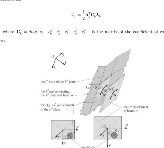
In the present paper it was assumed that the connection of electrodes and beams is made with the help of sde. Fig. 9 presents the connection of the electrode element with number k j i, , with
rfe e of beam . In structural solutions known to the author, there are always connections of
the need to take the rotation matrix into consideration in any further discussion. The vector of strain of sdeh may be described with the formula:
4
, , , 1
ses mes
h h e h k j i s
s
A q A q
Δ , (30)
where ses h
A , Amesh are matrices of 6 6 with constant coefficients. The strain energy may be described as:
T
1 2
h h h h
V Δ C Δ , (31)
where x y z
h diag ch ch ch ch ch ch
C is the matrix of the coefficient of connection stiff-ness.
Figure 9. Stiffness-damping connection h of element k j i, , of plate k with rfee of beam .
Differentiating (31) with regard to the generalised coordinates qe and qk j i s, , , , one may deter-mine the additional elements (matrices 6 x 6) that may be added to the stiffness matrix of electrode
( ) ( )
(1) (1)
( ) ( )
( ) ( )
( ) ( )
0 0 0 0
0 0 0 0
0 0 0 0
0 0 0 0
0 0 0 0
u u k k p p b b M M q M q M q M q M q q ( ) ( ) ( ) ( ) ( ) 1 (1)
(1) (1) (1)
( ) ( ) ( ) ( ) ( ) ( ) ( ) ( ) ( ) ( ) ( ) 1 0 0 0 0 0 0 0 0 u u
u u u
k p u b k k k k u b p p p u b
b b b b
k p
C
C C C C q
C C C q
q
C C C
C C C
C C C C
( ) (1) ( ) ( ) ( ) ( ) ( ) ( ) u k p p
b b b
q f
G
G
G
q G
q G Q
,
(32)
or in general form:
Mq Cq f. (33)
The equations of motion (33) were integrated with the Newmark method with a constant inte-gration step.
3 MODEL VERIFICATION AND VALIDATION
The FEM model presented in the previous chapter was implemented into VibroESPan calculation software. The verification presented in sub-chapter 3.1 is an indirect verification that consists of performing a simulation in the VibroESPan software and of comparing the results with those ceived when using the Abaqus commercial package. Validation is performed by comparing the re-sults of numerical simulations (achieved with the help of VibroESPan software) with the rere-sults of measurements on the test stand. The process of model validation is described in sub-chapter 3.2. Both during verification and validation, the system is loaded by gravitational force and the force impulse F(t) applied to the anvil.
Peak value WMax and root-mean-square value WRMSwere used to evaluate signals in the domain
of amplitudes. These values are expressed with the following relationships:
, , , 0max , ,
a
Max s s i s s i t t
1 2 2 , , , , ,
0
1 ta
RMS s s i s s i a
W a dt
t ,
(34b)
where ta is the time of analysis, s is the index that takes the value n if signal as s i, , was
deter-mined as the result of numerical calculations in the FEM model, or p if it was received in the ABQ
model (in the verification process), or if it was received as the result of measurements (in the vali-dation process), and i is the number of checkpoints. In the above formulae it was assumed that
, , s s i
a may be one of the following values:
, ,
, ,
2 2 , , , , , , , ,
, , , ,
- acceleration in the direction of axis , - acceleration in the direction of axis ,
- tangential acceleration in plane , - normal acceler
x s i
y s i
s s i s i x s i y s i
s i z s i
a
a
a a a a
a a
x
y
xy
2 2 2
, , , , , , , ,
ation to plane ,
- total acceleration,
c s i x s i y s i z s i
a a a a
xy
which means that s x y, , , ,c .
The verifiability indicators FAC2 were used as the error measure both in the process of verifica-tion and in the process of validaverifica-tion:
1 1 2 p n f i i p FAC N n (35a) , , , , , , 1
1 for 2
2
0 otherwise
i i
i i
s n s n f
i s p
s p
W a
N W a (35b)
where , ,
i
s s
W and , , i
s s
W are calculated in accordance with (34), Max RMS, , and np is
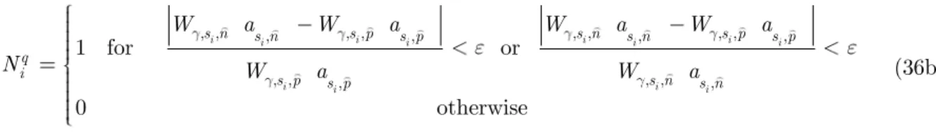
the number of checkpoints. The hit rate q a( )s is defined as:
1
1 np
, , , , , , , , , , , ,
, , , , , ,
1 for or
0 otherwise
i i i i i i i i
i i i i
s n s n s p s p s n s n s p s p
q
i s p s n
s p s n
W a W a W a W a
N W a W a (36b)
where is the allowable error.
3.1 Computational verification
The FEM model presented in Fig. 10 was applied during the remaining stages of verification and validation. The configuration of checkpoints presented in Fig. 10 corresponds to the arrangement of acceleration sensors on the test stand. Verification of the model with indicators FAC2 and q is exe-cuted for np 28 checkpoints and = 0.4.
Figure 10. Model scheme with an electrode system used in verification and validation.
The values of the model’s indicators calculated with reference to the results obtained from the
Figure 11. Verification: indicators FAC2 as and q as .
The comparative analysis of amplitudes presents good conformity of both models in the scope of the WRMS values of accelerations, especially the values of total acceleration ac. In the latter case, in
86% of the checkpoints, the values of WRMS are within the acceptable range of hit rate qRMS ac
and as much as 97% within the permissible range of the value of the FAC2RMS ac indicator.
3.2 Measuring Validation
Verification carried out as described above allowed for an exclusion of errors in the implementation of algorithms applied in the presented model. However, a model verified with a positive result does not necessarily have to be a model that correctly describes a real object. That is why the second
stage of the model’s evaluation should be performed. This consists in validation that describes the
correctness of the model with reference to the results of the measurements. Validation is carried out by comparing the results of numerical simulations with the results of measurements achieved on the test-bench. Conformity of the model with the object is performed by analysing the WMax as s, and
, RMS s s
Figure 12. Validation: indexes FAC2 as and q as .
High values of verifiability index FAC2 are obtained. For FAC2Max a , only 2 checkpoints
are not within the acceptable range, whereas in the case of index FAC2RMS ac – only one
check-point was outside the range. The values of index q as look slightly worse – in this case the dif-ferences in the values fluctuate between 4% and 25% (1 to 7 points). Such difdif-ferences may result from the fact that the acceleration measurements themselves are burdened with errors that result indirectly or directly from the accuracy of the sensors, linearity and distortions generated by the recorder in the output signal, from the precision of positioning the sensors in the test stand, accu-racy of signal synchronisation in the measurement sequences and accuaccu-racy of measurements of the force impulse. In addition, simplifications in the modelling of electrodes can be the reasons for the differences in calculations and measurement results.
4 CONCLUSIONS
The procedure applied in the present paper, in which sub-systems (beams and electrodes) are con-nected not with the help of equations of constraints, but through stiffness-damping elements, has its advantages and disadvantages. An advantage is the fact that there is no need to define additional
unknowns (Lagrange’s coefficients – constraint reactions). Its disadvantage is the lack of a general method of selecting the translation and rotational stiffness coefficients, sde, that join the sub-systems.
The results of verification and validation of the model allow to state that the model correctly re-flects the dynamic phenomena that appear in the system of collecting electrodes during the vibra-tions generated in them by an impulse of the force coming from the hammer of the rapping system. This verification and validation demonstrates some differences between the model and measurement results, but they are within the range of values accepted in engineering practice. Moreover, the re-sults are characterised by precision comparable to the precision achieved in commercial models, yet reached at considerably smaller computational costs [11]. Computer implementation of the model, as presented in the paper, has found application in the design office of one of Poland’s producers of electrostatic precipitators.
The overall conclusion is that the process of vibration excitation and wave propagation in the sys-tem of electrodes is the result of many factors [14]. This process depends not only on the impact force, but also on the physical parameters, geometry and construction of all the elements that make up this system [10]. In this respect the model presented in this paper is an important novelty, since using the testing calculations can help predict the properties of a future structure as early as in its design stage.
The author is aware of the imperfections in the presented models and results. It is the author’s opinion that future research should take into consideration:
developing a method of choosing the coefficients of stiffness of the collecting electrode connec-tions and beams, or replacing them with constraint equaconnec-tions,
applying the wave equations for the analysis of phenomena occurring in the system of the col-lecting electrodes.
Acknowledgements
This paper is an extended version of a speech delivered at the 11th Conference on Dynamical Systems – Theory and Applications, 5–8 December, 2011, in Łódź, Poland.
References
[1] Y. Yamamoto. Effects of Turbulence and Electrohydrodynamics on the Performance of Electrostatic Precipita-tors. Journal of Electrostatics, 22:11-22, 1989.
[2] Z. Long, Q. Yao, Q. Song, and S. Li. A second-order accurate finite volume method for the computation of elec-trical conditions inside a wire-plate electrostatic precipitator on unstructured meshes. Journal of Electrostatics. 67(4):597-604, 2009.
[3] S.L. Francis, A. Bäck, and P. Johansson. Reduction of Rapping Losses to Improve ESP Performance. Proceedings ICESP XI, Hangzhou, China; 2008.
[4] M. Sarna. Self exploring ESP rapping optimisation system. Proceedings ICESP VI, Budapest, Hungary, 1996. [5] A. Nowak, and S. Wojciech. Optimisation and experimental verification of a dust-removal beater for the
elec-trodes of electrostatic precipitators. Computers and Structures, 82(22):1785-1792, 2004.
[6] S.H. Kim, and K.W. Lee. Experimental study of electrostatic precipitator performance and comparison with exist-ing theoretical prediction models. Journal of Electrostatics, 48:3-25, 1999.
[7] L. Buhl, S. Drue, and L. Lind. Field testing of acoustical cleaning of electrostatic precipitators. Proceedings ICESP VI, Budapest, Hungary, 1996.
[8] O.C. Zienkiewicz, R.L. Taylor, and J.Z. Zhu. The finite element method: its basis and fundamentals. 6th ed., re-print, - Amsterdam : Elsevier Butterworth Heinemann, 2006.
[9] E. Wittbrodt, I. Adamiec-Wójcik, and S. Wojciech. Dynamics of flexible multibody systems. Rigid finite element method. Springer-Verlag Berlin Heidelberg, 2006.
[10] G. Rakowski, and Z. Kacprzyk. Metoda Elementów Skończonych w mechanice konstrukcji (Finite Element Method in mechanics of structures). Oficyna Wydawnicza PW, Warszawa, 2005 (in Polish).
[11] I. Adamiec-Wójcik, A. Nowak, and S. Wojciech. Comparison of methods for vibration analysis of electrostatic precipitators. Acta Mechanica Sinica, 27(1):72-79, 2011.
[12] J. Kruszewski et al. Metodasztywnych elementów skończonych w dynamice konstrukcji (Finite Element Method in dynamisc of structures). WN-T, Warszawa, 1999 (in Polish).
[13] M. Huang, Z. Zhao, and C. Shen. An effective planar triangular element with drilling rotation. Finite Elements in Analysis and Design, 46: 1031-1036, 2010.