J. Microw. Optoelectron. Electromagn. Appl. vol.10 número1

(1)

Numerical treatment of rounded and sharp

corners in the modeling of 2D electrostatic

fields

L. Krähenbühl, F. Buret, R. Perrussel, D. Voyer

Laboratoire Ampère (CNRS UMR5005); Université de Lyon, École Centrale de Lyon, France; e-mail: laurent.krahenbuhl@ec-lyon.fr

P. Dular

F.R.S.-FNRS, ACE research-unit; Université de Liège, Belgium; e-mail: patrick.dular@ulg.ac.be

V. Péron, C. Poignard

Team-Project MC2, INRIA Bordeaux-Sud-Ouest, Institut de Mathématiques de Bordeaux, CNRS UMR 5251 & Université de Bordeaux1, 351 cours de la Libération, 33405 Talence Cedex, France

e-mail: clair.poignard@inria.fr

Abstract_{— This work deals with numerical techniques to compute electrostatic} fields in devices with rounded corners in 2D situations. The approach leads to the solution of two problems: one on the device where rounded corners are replaced by sharp corners and the other on an unbounded domain representing the shape of the rounded corner after an appropriate rescaling. Both problems are solved using different techniques and numerical results are provided to assess the efficiency and the accuracy of the techniques.

Index Terms

—Finite element method, geometric singularity, asymptotic expansion, rounded corner.

I. Introduction

The precise description of an object containingrounded corners leads to consider meshes with a large number of nodes in the corner neighborhood when the finite element method (FEM) is straightforwardly applied. Dealing with such meshes makes the computation time- and resource-consuming. Moreover, these computations have to be repeated if the curvature radius of the rounded corner is modified.

In order to avoid this computational cost, the rounded corners are usually replaced by sharp corners. The obtained computational results are then “globally correct” but locally inaccurate in the neighborhood of the corners. We aim at remedying this drawback.

In this work, we are dealing with a 2D electrostatic problem in a domain with a rounded corner (see Fig. 1(a)). The proposed method to approximate the electric scalar potential is based on two observations, which can be checked by simple numerical experiments:

• the exact solutionsclose to the corner, computed for several values of the curvature radiusε, are quasi-similar, up to a “scaling factor” (related to ε). It is also noticed that the “shape” of the solutions close to the corner (their “shape” but not their amplitude) weakly depend on other elements of the studied structure, such as the distance to the boundaries: if the corner geometry isself-similar1_{, it is also said that the dominant term of the solutions close}

1

Roughly, it means that a single parameter, hereε, and a basic geometry are sufficient to describe the corners for any value ofε_{. For a precise definition, refer to [2].}

Journal of Microwaves, Optoelectronics and Electromagnetic Applications, Vol. 10, No. 1, June 2011 66

(2)

to the corner are self-similar.

• the exact solutions far from the corner are weakly influenced by the change of the curvature radius ε, and they converge to the solution on the domain with the sharp corner when ε goes to zero.

It can be deduced that an accurate approximate solution of the exact solution for any curvature radius εcan be build from the solutions of two problems:

• an electrostatic problem on the real domain except that the rounded corner is replaced by a sharp corner;

• an electrostatic problem on a domain that only takes the shape of the rounded corner into account. The corresponding solution so-called profile solution will be used with an appropriate “scaling”.

This intuitive argument coincides with the mathematical results proposed partially by Timouyas [1] in 2003 and recently completed by Dauge and her collaborators [2]. In addition to the predictable behavior of the solution, some error estimates are also provided in [1], [2] for the approximate solutions we consider. The method consists in matching the solutions of both problems. The main insight lies in this coupling: if the corner shape is modified (more than by the scale factor ε), then the only profile terms have to be computed again, leading to a gain in the computations compared with an entire re-meshing of the entire domain.

This work is addressed to the community of engineers that use numerical methods (as it was done in [3]), and the aim is to illustrate the finite element implementation of the theoretical concepts which are proved in other references [4], [2].

In Section II are given the principles of the method. Then, we provide explicitly how to solve the different problems that enable to build the approximate solution:

• the computation of the “singularity factor” of the solution on the domain with the sharp angle, in Section III;

• the problem on the unbounded domain taking only into account the shape of the rounded corner, in Section IV.

In Sections II, III and IV, numerical results are given to assess the accuracy of the proposed techniques.

II. Principles of the method

For the sake of clarity, the method is explained on a specific structure, see Fig. 1, but it can be straightforwardly extended to other structures, in particular including more than two electric conductors.

A. Definitions of the considered problems

Denote by v_ε the solution on Ω_ε (see Fig.1(a)) of the following problem:

     

    

△vε= 0, on Ωε,

vε= 0, on Γ0ε, and vε=V1, on Γ1,

∂vε

∂n = 0, on Γ N_,

(1)

(3)

O

r

θ

ω

Ω

_ε

ε

Γ

0 ε

Γ

0 ε

Γ

1

Γ

1

Γ

N

Γ

N

(a) Domain with a rounded corner Ωε.

O

r

θ

ω

Γ

0

Γ

0

Γ

1

Γ

1

Ω

Γ

N

Γ

N

(b) Domain with a sharp corner Ω.

O

ω

Ω

∞

1 Γ

0 ∞

r

∞

θ

(c) Unbounded profile domain Ω∞.

Figure 1. Considered domains Ω, Ω∞ and Ωε.

where n is the unitary outward normal on the boundary of the domain. The factor ε defines the true size of the rounded corner, starting from the profile domain given Fig. 1(c), where the characteristic size of the rounded corner is 1.

Let also v denote the solution on the domain Ω (see Fig. 1(b)) of a problem similar to (1):

          

△v= 0, on Ω,

v= 0, on Γ0, and v=V1, on Γ1,

∂v

∂n = 0, on Γ N_.

(2)

In the neighborhood of the sharp corner2_, _v _{can be expanded in series as follows [5]:}

v(r, θ) =λrαsin(αθ) + ∞ X

k=2

akrkαsin(kαθ),

α= π ω

, (3)

and the first term of this expansion is said singular because it makes the amplitude of the electric field go to the infinite at the sharp corner for α < 1 (i.e. ω > π). The factor λ is called the singularity factor in the following. Methods for the computation ofλ are given in Section III. A specific notation will also be used for the first function of expansion (3):

S(r, θ) =rαsin(αθ). (4)

Finally, let v∞ denote the solution of △v∞ = 0 in the unbounded domain Ω∞ where the characteristic size of the rounded corner is 1, see Fig. 1(c). The rounded corner has the same shape as in the real domain Ωε, the potential is zero on Γ0∞, and the behavior of the potential at infinity is given by the first term of the expansion (3) up to the scalarλ:

lim r∞→+∞

(v∞(r∞, θ)−S(r∞, θ)) = 0. (5)

The FEM enables to compute the term v∞ whatever the rounded corner shape (see Section IV). Note that for particular rounded corner shapes analytic expressions ofv∞ can be obtained, for instance using conformal maps.

2

It is valid on any intersection of a disc centered inOwith the domain Ω which coincides with the intersection of the same disc with an infinite sector whose corner is inO_{and whose angle is}ω_.

(4)

It is assumed in the remainder of this section that the approximate finite element solutions for v and v∞ have already been computed.

B. Proposed approximate solution

Solution vε can be computed straightforwardly by the FEM, using a “fine” discretization close to the rounded corner. However, this computation has to be performed for each corner “scale”ε.

Our aim is to approximate the solution vε by using only:

• the solution v, that will approximate v_ε far from the corner,i.e. whenr≫ε;

• the solution v∞ after a proper scaling by ε and the singularity coefficient λ, that will approximate the solution close to the corner, i.e. _when_r_≤_ε_.

The “scaling” used to map a point of polar coordinates (r, θ) in Ωε to a point in Ω∞ is given by (r∞, θ) = (r/ε, θ). This change of coordinates applied in (4) leads to:

εαS(r∞, θ) =S(r, θ). (6)

These considerations enable to understand the following approximate expressions, that are de-tailed in [2]:

v_ε(r, θ)≈λεαv∞(r∞, θ), for r < kε(usually, k= 1), (7)

vε(r, θ)≈v(r, θ) +λεα[v∞(r∞, θ)−S(r∞, θ)], (8)

for r > kε.

C. Remarks

The proposed expressions remain approximate:

• expressions (7) and (8) are not equal for r = kε, in particular when the geometry of the domain Ωε makes the solution for r < kε not to be symmetric with respect to θ=π/(2α). Indeed, in this first order approximation, the effect of the domain Ωε close to the corner is only related to the value of the singularity factorλ. It is not sufficient: any problem with the same angle ω and the same λ will give the same approximate solution close to the corner. A numerical example is considered in Subsection IV-D.

• in (8), (v∞(r∞, θ)−S(r∞, θ)) is not exactly zero on Γ1: thus, the conditions on this boundary, which are satisfied byv, are not satisfied by approximation (8). However, it can be seen, that whenever εgoes to zero, the remaining error becomes negligible: the scaling of the domain makes to send the boundaries further from the origin in the dimensionless solution v∞ and the behavior at infinity (5) can be used.

It is possible to compute complementary terms, to increase the accuracy of the approximate solution. In particular, the following term in the expansion (3), which varies as sin(2αθ), will be able to introduce an asymmetry of the approximation close to the rounded corner. Nonetheless, our numerical experiments with the first terms of the expansion show the relevance of this first order approach and illustrate the theoretical estimates for the numerical error [2].

We emphasize that the method is generic and could be applied to other particular shapes which would not be “rounded” (and even to a simple surface irregularity on a surface plane; see examples in [2]).

(5)

D. Application to the computation of the maximum field as a function of the curvature radius

With a reduced amount of numerical computations (a mesh of the whole studied device without the rounded corner and a mesh of the rounded corner but built independently from the rest of the structure) it is possible to determine the variation of the electric field close to the rounded corner as a function of the curvature radius. Indeed, the electric field E_ε(r, θ) in any point close to the rounded corner depends only on:

• the singularity factor λ whose evaluation is introduced in Section III starting from v, the solution with the sharp corner;

• the field E∞(r∞, θ) transferred to the domain Ω_ε;

• the scale factor ε.

The corresponding relation is given close to the corner by:

Eε(r, θ) =−grad(vε)(r, θ) =λε(α −₁₎

E∞(r∞, θ). (9)

For instance, if the statistical distribution of the curvature radii is known for a series of N pieces used in a high-voltage device, it will be possible to compute the statistical distribution corresponding to the maximal electric field in these pieces.

III. Computation of the singularity factor

A. The Fourier method: weighted line integral of v

The Fourier method enables to compute an approximation of the singularity factorλ from the solution v of the problem with the sharp corner (see Fig. 1(b)) given by the FEM. A weighted integral of v is computed on an arc of circle of radius r0 centered on O, from one border of the angle to the other:

λ= 2 ωr

−_α

0

ω Z

0

v(r0, θ) sin(αθ)dθ. (10)

Relation (10) is obtained by considering expansion (3) in the line integral. Whenθ varies between 0 and ω, αθ varies between 0 andπ; in this range of variation, the integration of sin(αθ) with sin(kαθ) is zero for all k strictly greater than 1.

There is no restriction in the choice of r0 except that the arc of circle must belong to the domain Ω.

B. Dual solution method

The theoretical explanations concerning this method can be found in [1, Subsubsection 2.3.8]. This approach enables to compute the singularity factor λ as follows:

λ= Z

Ω

f v∗

ds, (11)

where Ω is the domain with the sharp angle (see Fig. 1(b)),v∗

a function that is described in the following, and f a function equal to △w, where w is a “regular lifting” function. It is proposed here not to construct this “regular lifting” but the less regular lifting which is commonly (but often implicitly) used in the FEM.

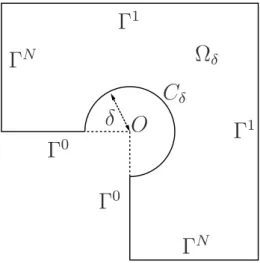
Consider a domain Ωδ, see Fig. 2. It can be seen that when the radius δ of the circle Cδ goes to zero, Ωδ converges to Ω, see Fig. 1(b).

(6)

O

C

δ

Γ

0

Γ

0

Γ

1

Γ

1

Γ

N

Γ

N

Ω

_δ

Figure 2. Domain Ωδ whereδ_→0 is considered.

For two functions v and v∗

in Ω_δ such that △v=△v∗

= 0 in Ω_δ, straightforward application of Green formula leads to

0 = Z

∂Ωδ _∂v

∂nv ∗

−v∂v ∗

∂n

dl, (12)

As in [1], integral (12) can be made explicit on each boundary of the domain for a non zero δ. Using the particular properties of the functions v andv∗

, and passing to the limit whenδ goes to zero lead to the result.

In this computation, v is the FEM solution of problem (2) on Ω. The function v∗

is the sum of the “dual singular function” S∗

:

S∗

(r, θ) =r−α

sin(αθ), (13)

and a more regular functionv∗

R computed on the domain Ω which is the solution of the following problem:           

△v∗

R= 0, on Ω,

v∗ R=−S

∗

, on Γ0∪Γ1, ∂v∗

R ∂n =−

∂S∗ ∂n , on Γ

N_.

(14)

Problem (14) can be solved by the FEM. Thus v∗

is the non zero singular function expressed by

v∗ =v∗

R+S ∗

. (15)

Let us note that this function satisfies

          

△v∗

= 0, on Ω,

v∗

= 0, on Γ0∪Γ1, ∂v∗

∂n = 0, on Γ N_,

(16)

but this problem cannot be solved by a classical variational approach.

Considering again the path integral (12) when δ goes to zero, the integration is restricted to

(7)

Γ1 andCδ:

0 = lim δ→0 Z

∂Ωδ _∂v

∂nv ∗

−v∂v ∗

∂n

dl,

= lim δ→0 Z

Γ1

−v∂v ∗

∂n dl+ limδ→0 Z

Cδ _∂v

∂nv ∗

−v∂v ∗

∂n

dl.

(17)

It can be shown that the path integral onCδ converges to πλwhen δ goes to zero:

lim δ→0 Z

Cδ _∂v

∂nv ∗

−v∂v ∗

∂n

dl=πλ. (18)

Moreover, the integral on Γ1 _{in (17) can be written:}

Z

Γ1

−v∂v ∗

∂n dl=−V

1Z Γ1

∂v∗

∂n dl. (19)

It is an integral only on the boundaries with non zero Dirichlet conditions (that are far from the corner), and it corresponds to the flux of the dual solution v∗

on each of these boundaries. The singularity factor is then given by:

λ=−1

πV

1Z Γ1

∂v∗

∂n dl. (20)

Integral (19) is a “classical” computation in the FEM that is often approximated by using Green formula by a surface integral:

−V1 Z

Γ1 ∂v∗

∂ndl≈V

1Z CΓ1

∇w· ∇v∗

ds, (21)

where CΓ1 _{is a transition layer often limited to one layer of elements in direct contact with the} boundary andwis equal to 1 on Γ1 and goes to zero through the layer; see Fig. 3 for the function w used in a FEM computation.

In fact, V1_w _{is the FEM lifting and it can be seen as an application of (11), by taking the} laplacian of V1_w _{as a distribution. Eventually, the singularity factor is given by}

λ=−1

πV

1Z

CΓ1∇w· ∇v ∗

ds. (22)

Figure 3. Lifting functionwused in a FEM computation.

(8)

C. Numerical comparison of both methods

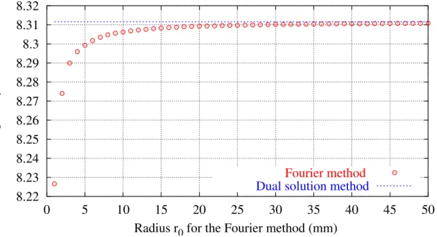
The singularity factor λ is computed on the geometry of Fig. 4. The boundary conditions are the same as these described in Subsection II-A. The potential V1 _{is chosen equal to 1.}

50mm

50mm 50mm

50mm

Figure 4. Domain for the computation ofλ_.

It is shown on Fig. 5 that for the method proposed in Subsection III-A, the computed result forλis dependent on the choice ofr0. Asr0increases, the computed value forλquickly coincides for both methods.

8.22

8.23

8.24

8.25

8.26

8.27

8.28

8.29

8.3

8.31

8.32

0

5

10

15

20

25

30

35

40

45

50 Singularity factor

Radius r

₀

for the Fourier method (mm)

Fourier method

Dual solution method

Figure 5. Value ofλ_{computed by the method described in Subsection III-A as a function of}r0. The dotted line indicates the value computed by the method described in Subsection III-B.

IV. Solution of the problem in _Ω∞

It was introduced in Subsection II-A a potential v∞ solution of the Laplace equation on the unbounded domain Ω∞.

(9)

In Subsection IV-A, the problem for v∞ is formulated as a classical Laplace problem with non homogeneous boundary conditions, straightforwardly solved by the FEM. In Subsection IV-B, it is shown that conformal maps may give a solution for certain specific shapes of the rounded corner. In Subsection IV-C, the practical method used to obtain the approximation (8) by combining the solutionv∞ with the solutionv on the domain with the sharp corner, is explained.

A. The equivalent problem with shifted singularity

Let us define a new functionS∞, with the correct behavior at infinity (5) and whose laplacian is zero in Ω∞. Note thatS (given in (4)) itself is not suitable, because its laplacian is not defined in O (r equal to 0). We propose for instance:

S∞(r, θ) =r_sαsin(αθ), (23)

wherersis the distance between the observation point and any point inside the infinite conductor, typically the center of curvature of the rounded corner (Fig. 6).

O

Γ

0

∞

r

_∞

r

_s

Figure 6. Definition ofrs

The behavior at infinite obviously satisfies (5), but this function is not zero on the surface of the conductor: v∞ will be written as the sum of this function S∞ and a corrective potential v_R∞_s:

v∞=S∞+vR∞s (24)

which is the solution of:     

   

△vR∞s= 0, on Ω∞,

vR∞_s=−S∞, on Γ0∞,

lim r∞→∞

vR∞s(r∞, θ) = 0.

(25)

This regular potential vR∞_s can be found with the FEM and a classical “shell transformation” in order to take the unbounded domain into account [6].

B. Method of conformal maps

The method of conformal maps [7] allows to build analytically potentials with the properties requested forv∞,i.e._{equal to zero on the conductor and with a prescribed behavior at infinity, on}

domains like Ω∞. However, only some particular shapes can be analyzed by these transformations.

(10)

1) Example of transformation for a rounded corner: Let us consider the two complex planes:

z=x+ iy=reiθ where (x, y) are the coordinates in the real geometry, (26)

w =u + iv =Reiφ where v is the electric potential. (27)

and the following conformal map [8, p. 320]:

z =k[(w +a)1/α+ (w−a)1/α], (28)

with a= 2α−₁

and k= 1/2.

The image of the straight line v = 0 in the w-plane is composed of (see Fig. 7):

• the half-line y= 0,x >1, for u> a(u−a >0 and u +a >0);

• the half-line reiπ/α, r >1, for u<−a (u−a <0 and u +a <0);

• a rounded line from P_l(z_l= eiπ/α) to P_r(z_r= 1), for u∈[−a, a], (u−a <0 and u +a >0).

Moreover, for |w|≫ |a|, z ≈ w1/α _{and v =} _ℑ_{(w) =}_R_sin(_φ₎ _≈_rα_sin(_αθ_{), what is the expected} behavior at infinity. Then, this transformation gives the solution v∞ for the particular shape given by (28), which is not exactly an arc of circle. We emphasize that this transformation does not lead to the exact computation of thev∞ corresponding to the previous subsection IV-A since the geometries are slightly different. However the solutions are similar as shown by the numerical simulations in Section IV-D.

Figure 7. z(u = constant) andz(v = constant) plotted in thez-plane for the conformal map (28). The rounded corner is not an arc of circle sincerr= 1,r0=

√

2−.5<1

(11)

2) Reference values of the electric field: The electric field on the conductor, for any point on the right of the rounded corner (v= 0, u> a) is:

−dv

dy =

−2α

(u +a)(1−α)/α_{+ (u}₋_a₎(1−α)/α. (29)

For example, the modulus ofE∞ at the ends of the rounded corner is

|E∞(Pl)|=|E∞(Pr)|=α2α, (30)

while on the middle-point of the rounded corner it equals

|E∞(P0)|=

α2(1−α)2/α

sin ₂π_α . (31)

For the right angle (α= 2/3), the field is constant on the rounded corner:

|E∞(α= 2/3, ε= 1)|= 25/3/3 = 1,058267... (32)

even though it varies for other parts of the conducting corner.

The approximate field on the real structure at the same points is deduced fromE∞ using (9): for this computation, only the scaleε and the singularity factorλ are required.

We propose to use the reference field (31), or its particular value 1.06 for a right rounded angle, when the shape of the rounding is not exactly known, and when an approximation of the maximum field as function of the mean curvature of the corner is the requested information.

3) Remarks: Such conformal maps have the required behavior at infinite and on the straight parts of the conductor for favorably replacing the singular function S∞ given in (23) used in Subsection IV-A. The only condition is that the linev= 0 remains inside the real conductor (at the reference scale ε = 1). By the way, the norm of the correction v_R∞_s (25) will probably be reduced.

C. Scaling by ε: projection method

Whatever the method used to build v∞ in the domain Ω∞ (the FEM, conformal maps or another method), this potential is not directly obtained on the mesh where v is computed.

Moreover, the computation of the sum (7) and (8) for a particularε, on a domain Ω_ε, see Fig. 1(a), requires a projection ofv∞ on the mesh of the final domain, with a scaling factor different for each value of ε. For this purpose, the projection is performed by a continuous least-square approach [9].

When only the results in some particular points is of interest, such as the amplitude of the electric field in the middle of the rounded corner, this step requires no particular computation.

D. Numerical results

The aim of the section is to illustrate the efficiency of the proposed method by computing the potential for two different domains: a symmetric configuration (the domain of Subsection III-C) and a non-symmetric configuration. The non-symmetric configuration consists in cutting down half vertical part of the symmetric domain (see Fig. 8(a)), the shape of the corner remaining the same in both cases.

(12)

50mm

d=25mm 50mm

50mm

(a) With the sharp corner.

ε= 20 mm

d=25mm

(b) With the largestε_considered.

Figure 8. Non-symmetric domain.

In addition we aim at studying the robustness of the approach by performing the numerical simulations for quite large corners. It is shown that even if the corner is large, the method provides good approximation of the potential in the symmetric configuration. For large corner, the accuracy of the method gets down in the non-symmetric configuration, but as soon as the corner becomes small compared with the characteristic size of the domain, the accuracy of two configurations reaches the same order ε.

Observe that since the corner shape is the same for both configurations, the profile termv∞ is the same. It is computed by considering the method proposed in Subsection IV-A. More precisely, the value of max(|E∞|) is 1.147 V/m (this value can be compared to the value 1.058 V/m that is given by the conformal map described in Subsection IV-B; the value given by the conformal map is equal, by keeping 4 significant digits, to the average value on the rounded corner that equals 1.058 V/m). For both problemsλis computed by the method proposed in Subsection III-B. In the symmetric configurationλ is equal to 8.312 (Fig. 4) while it equals 11.28 for the non-symmetric domain (Fig. 8(a)).

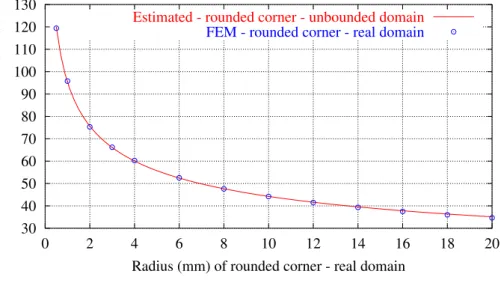
1) Electric field close to the corner in both configurations: According to relation (7) and (9) the knowledge of λ and v∞ should provide accurate approximation of the normal electric field on the conductor close to the corner. Fig. 9(a) provides the maximum values of the electric field given by the real problem (the domain with the rounded corner) and by the profile term in the unbounded domain for several corner radii in the symmetric configuration. Observe the good agreement between results obtained by formula (9) and results obtained by straightforward FEM computations even for large radii. In the non-symmetric domain, the accuracy of the approximation is slightly altered for large radii (see Fig 9(b)) But as soon as the radius is small compared with the characteristic size of the domain, the accuracy is similar to the symmetric domain. However we emphasize that even for large radii, the maximal values of the electric field in the non-symmetric configuration remain good, since the corresponding relative errors are smaller than 4% for a corner radius equal to 10mm (that is 40% of the domain characteristic size).

(13)

30 40 50 60 70 80 90 100 110 120 130

0 2 4 6 8 10 12 14 16 18 20

Maximum electric field (V/m)

Radius (mm) of rounded corner - real domain Estimated - rounded corner - unbounded domain

FEM - rounded corner - real domain

(a) Symmetric case

40 60 80 100 120 140 160

0 2 4 6 8 10 12 14 16 18 20

Maximum electric field (V/m)

Radius (mm) of rounded corner - real domain Estimated - rounded corner - unbounded domain

(b) Non-symmetric case

Figure 9. Comparison of the maximum electric field on the rounded corner between results obtained by straightforward FEM computations and results obtained by relation (9).

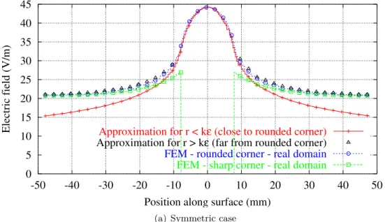
2) Electric field far from the corner: Function v and relation (8) should provide accurate approximations of the normal electric field on the conductor far from the corner for the symmetric and non symmetric domains. This is recovered by the simulations (see Figs. 10(a), 10(b), 11(a) and 11(b)).

Observe that for small values ofεin the non symmetric domain (the corner radius equals 2 mm and 1 mm respectively in Fig.11(a) and in Fig. 11(b)) the point-wise difference between the real and the approximate electric field near the corner is improved compared to Fig. 10(b).

V. Conclusion and perspectives

In this work, a set of practical techniques was proposed to enable the implementation of new methods to estimate the electric field in the neighborhood of conductors containing rounded

(14)

0 5 10 15 20 25 30 35 40 45

-50 -40 -30 -20 -10 0 10 20 30 40 50

Electric field (V/m)

Position along surface (mm)

Approximation for r < kε (close to rounded corner)

Approximation for r > kε (far from rounded corner)

FEM - sharp corner - real domain

(a) Symmetric case

0 10 20 30 40 50 60

-50 -40 -30 -20 -10 0 10 20 30 40 50

Approximation for r < kε_{(close to rounded corner)} Approximation for r > kε_{(far from rounded corner)} FEM - rounded corner - real domain FEM - sharp corner - real domain

(b) Non-symmetric case

Figure 10. Comparison of the normal electric field on the conductor forε= 10 mm.

corners, in the 2D case.

The computation on the whole studied structure can be done by replacing rounded corners by sharp corners. A generic self-similar solution enables to estimate the electric field close to the corner by post-processing for several values of the curvature radius. Some numerical tests have assessed the relevance of the proposed approach.

It has been also shown that forgotten techniques, as conformal maps, enable, in some cases, to build exactly the generic solution and in every case, to approximate it. They can be coupled with more computationally intensive numerical methods as the FEM, by providing speed and accuracy.

(15)

0 20 40 60 80 100

-10 -8 -6 -4 -2 0 2 4 6 8 10

Approximation for r > kε (far from rounded corner)

(a)ε_{= 2 mm}

0 20 40 60 80 100 120

-5 -4 -3 -2 -1 0 1 2 3 4 5

Approximation for r > kε_{(far from rounded corner)}

(b) ε= 1 mm

Figure 11. Comparison of the normal electric field on the conductor for the non-symmetric case Fig. 8(b).

ε_{= 2 mm and}ε_{= 1 mm.}

(16)

We are currently working to the extension of these techniques to:

• cases with several angles (such as some MEMs applications),

• 3D cases which is our real aim,

• singularity treatment (with sharp corners) for eddy-current problems, that lead also to self-similar solutions, with the penetration depth δ playing the same role as the scaling factorε in the present study.

VI. Acknowledgments

This work was partially supported by ANR (ANR-06-BLAN-0417).

The authors have a grateful thought for Michelle Schatzman who left us recently. Her love for mathematics and their applications was a true moving spirit for this collaboration. The authors would like to dedicate this work to her memory.

References

[1] H. Timouyas, “Analyse et analyse numérique des singularités en électromagnétisme,” Ph.D. dissertation, Ecole Centrale de Lyon, 2003. [Online]. Available: http://tel.archives-ouvertes.fr/tel-00110828.

[2] M. Dauge, S. Tordeux, and G. Vial,Around the Research of Vladimir Maz’ya II: Partial Differential Equations. Springer Verlag, 2010, ch. Selfsimilar Perturbation near a Corner: Matching Versus Multiscale Expansions for a Model Problem, pp. 95–134.

[3] L. Krähenbühl, H. Timouyas, M. Moussaoui, and F. Buret, “Coins et arrondis en éléments finis - Une approche mathématique des coins et arrondis pour les solutions par éléments finis de l’équation de Laplace,” RIGE, vol. 8, pp. 35–45, 2005.

[4] S. Tordeux, G. Vial, and M. Dauge, “Matching and multiscale expansions for a model singular perturbation problem,”Comptes Rendus Mathematique, vol. 343, no. 10, pp. 637–642, Nov. 2006.

[5] P. Grisvard,Elliptic problems in nonsmooth domains. Pitman Advanced Pub. Program, 1985.

[6] F. Henrotte, B. Meys, H. Hedia, P. Dular, and W. Legros, “Finite element modelling with transformation techniques,”Magnetics, IEEE Transactions on, vol. 35, no. 3, pp. 1434–1437, 1999.

[7] Wikipedia. Conformal map. [Online]. Available: http://en.wikipedia.org/wiki/Conformal_map

[8] E. Durand,Electrostatique, Vol. 2 : Problèmes généraux conducteurs. Editions Masson, Paris, 1964-1966. [9] C. Geuzaine, B. Meys, F. Henrotte, P. Dular, and W. Legros, “A Galerkin projection method for mixed finite

elements,”Magnetics, IEEE Transactions on, vol. 35, no. 3, pp. 1438–1441, 1999.