Abstract— General stress functions for determining the stress concentration around circular, elliptical and triangular cutouts in laminated composite infinite plate subjected to arbitrary biaxial loading at infinity are obtained using Muskhelishvili’s complex variable method. The generalized stress functions are coded using MATLAB 7.0 and the effect of fiber orientation, stacking sequence, loading factor, loading angle and cutout geometry on stress concentration around cutouts in orthotropic/anisotropic plates is studied.
Index Terms – Composites, cutouts, failure criteria, stress concentration factors, stress functions
I. INTRODUCTION
arious shaped cutouts are made in structures and machines to satisfy certain service requirements. These cutouts work as stress raisers and may lead to catastrophic failure. The behavior of isotropic plates with such cutouts, under different loading conditions is already studied extensively by many researchers. But, the anisotropic media with various shaped discontinuity has received very little attention.
Using Kolosov-Muskhelishvili’s [1] complex variable approach, some problems of simply connected regions are solved by Savin [2],Lekhnitskii [3], Ukadgaonker and Rao [4],[5], Ukadgaonker and Kakhandki [6], Nageswara Rao et al [7], Daoust and Hoa [8], Rezaeepazhand and Jafari [9] etc.
Savin [2] and Lekhnitskii [3] found stress concentrations around circular, elliptical, triangular and square holes, mainly in isotropic media. Though, Savin [2] used integro-differential approach and Lekhnitskii [3] used series approach to define the stress function, the final outcomes are same. The analytic solutions for stress analysis of infinite anisotropic plate with irregular holes are presented by Ukadgaonker and Rao [4],[5] and Ukadgaonker and Kakhandki [6]. They adopted Gao’s [10] arbitrary biaxial loading condition to eliminate superposition of two uniaxial loading problem to obtain solution for biaxial loading problem. Ukadgaonker and Rao [5] and Daoust and Hoa [8] presented solutions for stress distribution around triangular hole with blunt corners in composite plates, whereas Nageswara Rao et al [7] found stress field around square and rectangular holes.
In this paper, Kolosov-Mushkhelishvilli’s complex variable approach is adopted to obtain generalized stress functions. The effect of hole geometry, material properties, fiber orientation, stacking sequence, loading factor and loading
Dharmendra Sharma is with the Institute of Technology, Nirma University, Ahmedabad-382481, India (phone +91-2717-241911, ext 687 fax 91-2717-241911; email:[email protected] )
angle on stress field around cut-outs is studied. For numerical results Graphite/epoxy, Glass/epoxy and isotropic materials are considered.
II. COMPLEX VARIABLE FORMULATION
For thin anisotropic plate, using generalized Hooke’s law, Airy’s stress function and strain-displacement compatibility condition, the following characteristic equation is obtained, roots of which represents constant of anisotropy (Lekhnitskii [3]).
0
2
)
2
(
2
22 26
2 66 12 3
16 4
11
a
s
a
s
a
a
s
a
s
a
(1)
ij
a
are the compliance co-efficient. The roots of the equation (1) are;1 1 1
i
s
;s
2
2
i
2;1 1 3
i
s
;s
4
2
i
2 (2) The stress components for plane stress conditions can bewritten in terms of Muskhelishvili’s stress functions (
(
z
1)
and
(
z
2)
) and constants of anisotropy (s1 and s2), asfollows (Savin [2]):
'
(
)
'
(
)
Re
2
s
12z
1s
22z
2x
'
(
)
'
(
)
Re
2
z
1z
2y
(3)
'
(
)
'
(
)
Re
2
s
1z
1s
2z
2xy
)
(
'
z
1
and
'
(
z
2)
are the first derivatives of the Mushkhelishvili’s complex stress functions
(
z
1)
and)
(
z
2
, respectively.The stresses in Cartesian coordinates given in equation (3) can be written in orthogonal curvilinear coordinate system by means of the following relations
xy y x
n
m
mn
mn
mn
m
n
mn
n
m
2 2 2 2
2 2
2
2
(4)
m and n are the direction cosines.
III. MAPPING FUNCTION
The area external to a given hole (here, circular, elliptical or triangular), in Z-plane is mapped conformably to the area outside the unit circle in ζ plane using following mapping function.
Stress Concentration around
Circular/Elliptical/Triangular Cutouts in Infinite
Composite Plate
Dharmendra S Sharma, Member, IAENG
V
N k k km
R
z
1)
(
(5)0
k
m
, for circular hole
b
a
b
a
m
k
1
,
k , for elliptical hole, where, a and b are the semi major and semi minor axis of the ellipse, respectively...
17
,
14
,
11
,
8
,
5
,
3
k
andm
3
1
/
3
;m
5
1
/
45
;162
/
1
8
m
;m
11
7
/
2673
;m
14
1
/
729
;111537
/
91
17
m
, for triangular hole.For anisotropic materials, the deformations undergo affine transformation. Hence, the mapping function (equation (5)) is modified by introducing complex parameters
s
j.
N k k k j N k k k j j jm
b
m
a
R
z
1 11
2
)
(
1
j
,
j
is
a
b
j
1
is
j
; j=1,2. (6)IV. ARBITRARY BIAXIAL LOADING CONDITIONS In order to consider several cases of in-plane loads, the arbitrary biaxial loading condition is introduced into the boundary conditions. This condition has been adopted from Gao’s [10] solution for elliptical hole in isotropic plate. By means of this condition solutions for biaxial loading can be obtained without the need of superposition of the solutions of the uniaxial loading. This is achieved by introducing the biaxial loading factor λ and the orientation angle β into the boundary conditions at infinity.
Fig. 1 Arbitrary biaxial loading condition
The boundary conditions for in-plane biaxial loading conditions are as follows:
;
'
x
'
;
y '
0
xy
atz
Where,
x' and
'
y
are stresses applied about x`, y` axes at infinity (Refer Fig. 1). By applying stress invariance into above boundary conditions, boundary conditions about XOY can be written explicitly as:]
2
cos
)
1
(
)
1
[(
2
x
p
]
2
cos
)
1
(
)
1
[(
2
y
p
]
2
sin
)
1
[(
2
xy
p
(7) For inclined uniaxial tension: λ=0, β≠0(a) Loading along x-axis : λ=0, β=π/2 (b) Loading along y-axis : λ=0, β=0 For equi-biaxial tension : λ=1, β=0
For shear stress : λ=-1, β=π/4 or 3π/4
V. STRESS FUNCTION FOR CUTOUTS OF DIFFERENT SHAPES The scheme for solution of anisotropic plate containing a cutout subjected to remotely applied load is shown in Fig. 2. To determine the stress function, the solution is split into two stages:
A. First Stage
The stress functions
(
z
1)
and
(
z
2)
are determined for the hole free plate under the application of remotely applied load. The boundary conditionsf
1andf
2are found for the fictitious hole using stress functions
(
z
1)
and
(
z
2)
. The stress function
(
z
1)
and
(
z
2)
are obtained for hole free plate due to remotely applied load
x,
y as1 * 1
1
(
z
)
B
z
2 '* '* 2
1
(
z
)
(
B
iC
)
z
(8) Where,))
(
)
((
2
2
)
(
2 1 2 2 2 1 2 2 2 2 2 2 *
xy y xB
))
(
)
((
2
2
)
2
(
2 1 2 2 2 1 2 2 2 1 2 1 2 1 '*
xy x yB
)] ( ) [( 2 )] ( ) [( )] ( ) ( [ )] [( 2 1 2 2 2 1 2 2 2 2 2 2 2 1 2 1 2 2 2 2 1 2 1 2 1 2 2 1 '*
xy y x CThe boundary conditions
f
1,
f
2on the fictitious hole aredetermined from these stress functions as follows.
N k k k N k k km
K
K
m
K
K
f
1 1 2 1 2 1 1)
(
1
)
(
N k k k N k k km
K
K
m
K
K
f
1 3 4 1 4 3 2)
(
1
)
(
(9) Where,
2
'* '* 1 *
1
(
)
2
B
a
B
iC
a
R
K
2
'* '* 1 *
2
(
)
2
B
b
B
iC
b
R
K
2
'* '* 2 1 * 1
3
(
)
2
s
B
a
s
B
iC
a
R
K
2
'* '* 2 1 * 1
4
(
)
2
s
B
b
s
B
iC
b
R
K
B. Second Stage
For the second stage solution, the stress functions
)
(
10
z
and
0(
z
2)
are determined by applying negative of the boundary conditionsf
10
f
1 andf
20
f
2 on its hole boundary in the absence of the remote loading. The stress functions of second stage solution are obtained using these new boundary conditions(
f
10,
f
20)
into Schwarz formula:
t
dt
t
t
f
f
s
s
s
i
)
(
)
(
4
)
(
2 10 202 1 0
t
dt
t
t
f
f
s
s
s
i
)
(
)
(
4
)
(
1 10 202 1
0
(10) By evaluating the integral the stress functions are obtained as
N k k km
b
a
1 3 30
(
)
N k k km
b
a
1 4 40
(
)
(11)Where,
(
)
(
)
1
4 3 2 1 2 2 13
s
K
K
K
K
s
s
a
(
)
(
)
1
3 4 1 2 2 2 13
s
K
K
K
K
s
s
b
(
)
(
)
1
4 3 2 1 1 2 14
s
K
K
K
K
s
s
a
(
)
(
)
1
3 4 1 2 1 2 14
s
K
K
K
K
s
s
b
C. Final Solution
The stress function
(
z
1)
and
(
z
2)
for single hole problem, can be obtained by adding the stress functions of first and second stage.)
(
)
(
)
(
z
1
1z
1
0z
1
)
(
)
(
)
(
z
2
1z
2
0z
2
(12)(1) (2) (3) Fig.2.Problem configuration with scheme of solution
VI. RESULTS AND DISCUSSION
The numerical results are obtained for Graphite/epoxy (E1=181GPa, E2=10.3GPa, G12=7.17GPa and ν12=0.28) and
Glass/epoxy (E1=47.4GPa, E2=16.2GPa, G12=7.0GPa and
ν12=0.26). Some of the results are obtained for isotropic
plate (E=200GPa, G=80GPa and ν=0.25) also for sake of comparison. The steps followed in computer implementation are as under:
1. Choose the value of biaxial load factor, λ and load angle, β for the type of loading.
2. Calculate the compliance co-efficient, aij from
generalized Hooke’s Law.
3. Calculate the value of complex parameters of anisotropy s1 and s2 from the characteristic equation
(equation 1). Some of the constants of anisotropy s1
and s2 are presented in Table 1.
4. Calculate the constants:
a1,b1,a2,b2,B,B’,C’,K1,K2,K3,K4etc.
5. Evaluate the stress functions and their derivatives. 6. Evaluate stresses.
The following loading cases have been considered.
1. Plate subjected to uni-axial tension at infinite distance.
2. Plate subjected to biaxial tension at infinite distance.
Table 1 Constants of anisotropy Fiber
angle
Graphite/epoxy Glass/epoxy
s1 s2 s1 s2
0 -0.0000 +
4.8936i
0 + 0.8566i
0.0000 + 2.3960i
-0.0000 + 0.7139i
90 -0.0000 +
1.1674i
0.0000 + 0.2043i
-0.0000 + 1.4007i
0.0000 + 0.4174i
0/90 -0.0000 +
3.6403i
0.0000 + 0.2747i
-0.0000 + 2.0142i
0.0000 + 0.4965i
45/-45
-0.8597 + 0.5109i
0.8597 + 0.5109i
-0.6045 + 0.7966i
0.6045 + 0.7966i
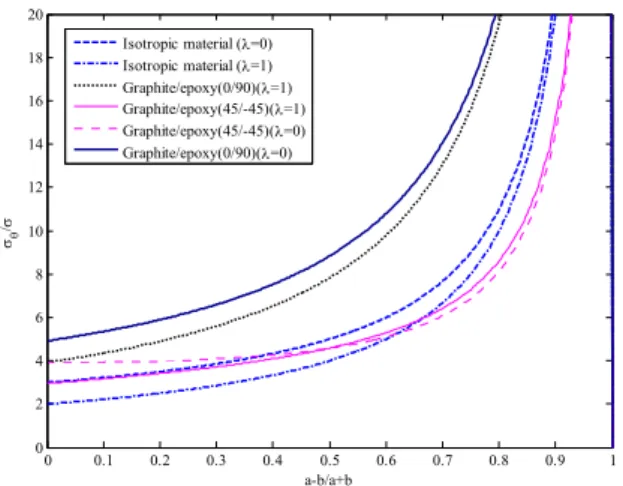
The stress concentration around elliptical hole varies as ratio of lengths of minor axis (2b) to major axis (2a) varies. The circle (b/a=1) and crack (b/a=0) are the special case of ellipse. As b/a approaches zero, the stress concentration at the end of major axis of the ellipse tends to be infinite for all materials (Refer Fig 3). For isotropic material the stress concentration is found higher when uni-axial load is applied compared to equi-biaxial loading.
0 0.1 0.2 0.3 0.4 0.5 0.6 0.7 0.8 0.9 1 0
2 4 6 8 10 12 14 16 18 20
a-b/a+b
/
Isotropic material (=0) Isotropic material (=1) Graphite/epoxy(0/90)(=1) Graphite/epoxy(45/-45)(=1) Graphite/epoxy(45/-45)(=0) Graphite/epoxy(0/90)(=0)
Fig. 3: Change in maximum stress concentration factor for elliptical hole as ratio of semi minor to semi major axis varies from 0(crack) to 1.0(circle).
The mapping function having 7 terms is used for triangular hole. As number of terms increases the hole shape converges to equilateral triangle and corner radius decreases. With the 7-term mapping function the corner radius is found 0.0031 with side length 2.3676.
Stress is a point function and varies as we go around the hole boundary. Fig. (4) shows the stress distribution around triangular hole for different materials (corner radius,
r=0.0476). The hole geometry and material parameters are taken same as Ukadgaonker and Rao [5] and Daoust and Hoa [8]. Fig. (4) can be compared with Fig. (3) (pp. 178) of Ukadgaonker and Rao [5] and Fig. (6) (pp. 127) of Daoust and Hoa [8].
0 20 40 60 80 100 120 140 160 180
-5 0 5 10 15 20 25
/
Isotropic Material CE9000 Glass/Epoxy Plywood
T300/5208Graphite/Epoxy
Fig. 4: Normalized tangential stress around the triangular hole (corner radius=0.0457, load angle, β=00, fiber orientation angle, Φ =00).
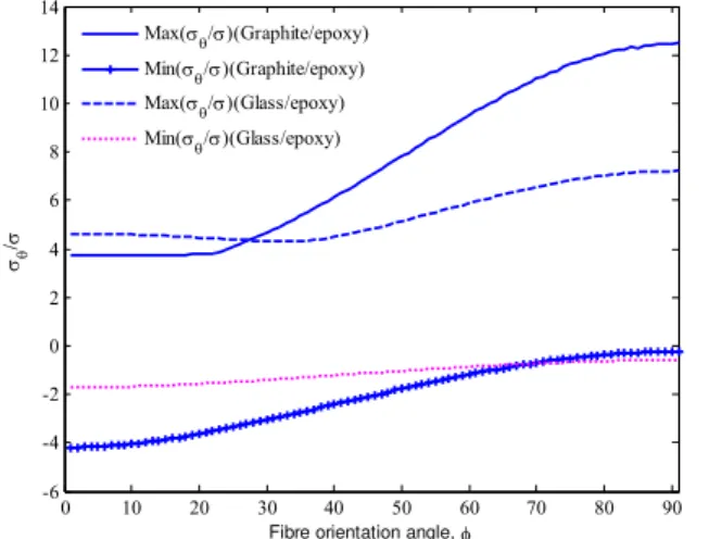
The Graphite/epoxy and Glass/epoxy lamina are considered to understand the effect of fiber orientation angle on normalized tangential stress. The maximum (σ/σ) on the
boundary of hole corresponding to fiber orientation angle ranging from 00 to 900 are shown in Fig. 5, 6 and 7. For plates with circular and elliptical hole the maximum tensile stress (σ/σ) increases as fiber orientation angle increases,
whereas maximum compressive stress (σ/σ) decreases
(Refer Fig 5 and 6). For the plate containing triangular hole the effect of fiber orientation angle (Φ) on normalized tangential stress (σ/σ) for Graphite/epoxy and Glass/epoxy
material is studied for load angle β=00 and β=900. The Graphite/epoxy plate subjected to uni-axial loading (=0, β=00) experience highest stress concentration when fiber orientation angle is Φ=900. (Refer Fig. 7)
0 10 20 30 40 50 60 70 80
-4 -2 0 2 4 6 8
Fibre orientation angle,
/
Max(/)(Graphite/epoxy) Min(/) (Graphite/epoxy) Max(/) (Glass/epoxy) Min(/) (Glass/epoxy)
Fig. 5: Effect of fiber orientation angle (Φ) on normalized tangential stress (σ/σ) for Graphite/epoxy and Glass/epoxy
0 10 20 30 40 50 60 70 80 90 -6
-4 -2 0 2 4 6 8 10 12 14
Fibre orientation angle,
/
Max(/)(Graphite/epoxy) Min(/)(Graphite/epoxy) Max(/)(Glass/epoxy) Min(/)(Glass/epoxy)
Fig. 6: Effect of fiber orientation angle (Φ) on normalized tangential stress (σ/σ) for Graphite/epoxy and Glass/epoxy plate with elliptical hole having a/b=2.0
0 10 20 30 40 50 60 70 80 90
20 30 40 50 60 70 80 90 100
Fibre orientation angle,
Ma
x
(
/
)
(Graphite/epoxy),=00
(Glass/epoxy),=00
(Graphite/epoxy),=900
(Glass/epoxy), =900
98.0271 75.9572
53.4750 40.2480
Fig. 7: Effect of fiber orientation angle (Φ) on normalized tangential stress (σ/σ) for Graphite/epoxy and Glass/epoxy
plate with triangular hole with corner radius=0.0031
The load angle (β) is varied from 00 to 900 and corresponding maximum normalized tangential stress is found. The effect of load angle (β) on maximum normalized tangential stress (σ/σ) for Graphite/epoxy and isotropic
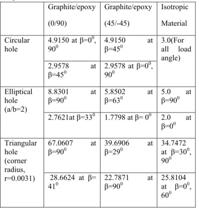
plate with circular, elliptical and triangular hole is presented in Fig. (8), (9) and (10), respectively. The maximum and minimum values of maximum normalized tangential stress corresponding to some load angle are tabulated in Table (2).
0 10 20 30 40 50 60 70 80 90
2.5 3 3.5 4 4.5 5
Load angle,
Ma
x
( /
)
Graphite/epoxy(0/90) Graphite/epoxy(45/-45) Isotropic material
Fig. 8: Effect of load angle (β) on maximum normalized tangential stress (σ/σ) for Graphite/epoxy and isotropic plate with circular hole
0 10 20 30 40 50 60 70 80 90
1 2 3 4 5 6 7 8 9
Load angle,
Ma
x
(
/
)
Graphite/epoxy(0/90) Graphite/epoxy(45/-45) Isotropic materials
Fig. 9: Effect of load angle (β) on maximum normalized tangential stress (σ/σ) for Graphite/epoxy and isotropic
plate with elliptical hole having a/b=2.0
0 10 20 30 40 50 60 70 80 90
20 25 30 35 40 45 50 55 60 65 70
Load angle,
/
Graphite/epoxy(0/90) Graphite/epoxy(45/-45) Isotropic material
Fig. 10: Effect of load angle (β) on maximum normalized tangential stress (σ/σ) for Graphite/epoxy and isotropic
Table 2. The stress concentration factors for various load angles.
Graphite/epoxy (0/90)
Graphite/epoxy (45/-45)
Isotropic Material Circular
hole
4.9150 at β=00, 900
4.9150 at β=450
3.0(For all load angle) 2.9578 at
β=450
2.9578 at β=00, 900
Elliptical hole (a/b=2)
8.8301 at β=900
5.8502 at β=630
5.0 at β=900
2.7621at β=330 1.7798 at β= 00 2.0 at β=00 Triangular
hole (corner radius, r=0.0031)
67.0607 at β=900
39.6906 at β=290
34.7472 at β=300, 900 28.6624 at β=
410
22.7871 at β=900
25.8104 at β=00, 600
VII. CONCLUSION
The general stress functions for determining the stress concentration around circular, elliptical and triangular cutouts in laminated composite plate subjected to arbitrary biaxial loading at infinity are obtained using Muskhelishvili’s complex variable method. The solution presented here can be a handy tool for the designers. From the numerical results following points can be concluded:
1. The principle of superposition can be avoided by introducing biaxial loading factor.
2. As the ratio of minor to major axis in elliptical hole decreases from 1.0 to 0, the stress concentration at the tip of major axis approaches infinity. The stress concentration factor for isotropic material under biaxial loading is always smaller than that obtained when uniaxial loading is applied.
3. The stress concentration factor is greatly affected by fiber orientation and loading angle.
4. The bluntness of the corner radius has significant effect on stress concentration.
REFERENCES
[1] N. I. Muskhelishvili, Some basic problems of the mathematical theory of elasticity. Groningen-P.Noordhooff Ltd, 1963.
[2] G. N. Savin, Stress concentration around holes. New York-Pergamon Press, 1961.
[3] S. G. Lekhnitskii, Theory of elasticity of an anisotropic elastic body. San Francisco-Holden-Day Inc, 1963. [4] V. G. Ukadgaonker and D. K. N. Rao, “A general
solution for stresses around holes in symmetric laminates under in-plane loading,” Composite Structure, vol. 49, pp. 339-354, 2000.
[5] V. G. Ukadgaonker and D. K. N. Rao, “Stress distribution around triangular holes in anisotropic plates,” Composite Structure, vol. 45, pp. 171-183, 1999.
[6] V.G. Ukadgaonker and V. Kakhandki, “Stress analysis for an orthotropic plate with an irregular shaped hole for different in-plane loading conditions-part-I.” Composite Structure, vol. 70, pp. 255-274, 2005.
[7] D. K. Nageswara Rao, M. Ramesh Babu, K. Raja Narender Reddy and D. Sunil, “Stress around square and rectangular cutouts in symmetric laminates,” Composite Structure, vol. 92, pp. 2845-2859, 2010. [8] J. Daoust and S. V. Hoa, “An analytical solution for
anisotropic plates containing triangular holes,” Composite Structure, vol.19, pp. 107-130, 1991.
[9] J. Rezaeepazhand and M. Jafari, “Stress concentration in metallic plates with special shaped cutout,” International Journal of Mechanical Sciences, vol.52, pp. 96–102, 2010.