Abs tract
This paper is devoted to the study of propagation of Rayleigh waves in a homogeneous isotropic microstretch generalized ther-moelastic diffusion solid half-space. Secular equations in mathe-matical conditions for Rayleigh wave propagation are derived for stress free, insulated/impermeable and isothermal/isoconcentrated boundaries. The phase velocity, attenuation coefficient, the com-ponents of normal stress, tangential stress, tangential couple stress, microstress, temperature change and mass concentration are computed numerically. The path of surface particles is also obtained for the propagation of Rayleigh waves. The computa-tionally stimulated results for the resulting quantities are repre-sented to show the effect of thermally insulated, impermeable boundaries and isothermal, isoconcentrated boundaries alongwith the relaxation times. Some particular cases have also been deduced from the present investigation.
Key words
Rayleigh waves; Frequency equation; Phase velocity; Attenuation coefficient; Microstretch
Rayleigh waves in isotropic microstretch thermoelastic
diffusion solid half space
1 INTRODUCTION
Eringen [1966, 1968] developed the theory of micromorphic bodies by considering a material point as endowed with three deformable directions. Subsequently, he developed the theory of microstretch elastic solid [1971] which is a generalization of micropolar elasticity [1966]. The material points in microstretch elastic body can stretch and contract independently of the translational and rotational processes. The difference between these solids and micropolar elastic solids stems from the presence of scalar microstretch and a vector first moment. These solids can undergo intrinsic volume change independent of the macro volume change and is accompanied by a non deviatoric stress moment vector.
Eringen [1990] also developed the theory of thermo microstretch elastic solids. The microstretch continuum is a model for Bravias lattice with a basis on the atomic level and a two phase dipolar solid with a core on the macroscopic level. For example, composite materials reinforced with
Raj n ee s h Kum ar*, a Sa nj e ev A h u jab S. K.G argc
a
Department of Mathematics, Kurukshetra University, Kurukshetra, Haryana, India
b
University Institute of Engg. & Tech., Kurukshetra University, Kurukshetra, Harya-na, India
c
Department of Mathematics, Deen Bandhu Chotu Ram Uni. of Sc. & Tech., Sonipat, Haryana, India
Received in 09 Mar 2013 In revised form 16 May 2013
chopped elastic fibres, porous media whose pores are filled with gas or inviscid liquid, asphalt or other elastic inclusions and ‘solid-liquid’ crystals, etc., should be characterizable by microstretch solids. A comprehensive review on the micropolar continuum theory has been given in his book by Eringen [1999].
Iesan and Pompei [1995] discussed the equilibrium theory of microstretch elastic solids. Propaga-tion of Rayleigh surface waves in microstretch thermoelastic continua under inviscid fluid loadings have been investigated by Sharma et. al.[2008]. Quintanilla [2002] also developed the spatial decay for the dynamic problems of thermomicrostretch elastic solid. The plane waves of generalized ther-momicrostretch elastic half space under three theories have been developed by Othman and Lot-fy[2010].The propagation of free vibrations in microstretch thermoelastic homogeneous isotropic, thermally conducting plate bordered with layers of inviscid liquid on both sides subjected to stress free thermally insulated and isothermal conditions have been investigated by Kumar and Pratap [2009]. In recent times, Kumar and Kansal [2011] construct the fundamental solution of system of differential equations in the theory of thermomicrostretch elastic diffusive solids in case of steady oscillations in terms of elementary functions.
The thermodiffusion in elastic solids is due to coupling of fields of temperature, mass diffusion and that of strain in addition to heat and mass exchange with the environment. Nowacki [1974,1976] developed the theory of thermoelastic diffusion by using coupled thermoelastic model. Dudziak and Kowalski [1989] and Olesiak and Pyryev [1995] respectively, discussed the theory of thermodiffusion and coupled quasi-stationary problems of thermal diffusion for an elastic layer. Uniqueness and reciprocity theorems for the equations of generalized thermoelastic diffusion prob-lem, in isotropic media, was proved by Sherief et al. [2004] on the basis of the variational principle equations, under restrictive assumptions on the elastic coefficients. Recently, Kumar and Kansal [2008] developed the basic equation of anisotropic thermoelastic diffusion based upon Green-Lindsay model.
Kumar and Kansal [2009] discussed the propagation of Rayleigh waves in a homogeneous trans-versely isotropic, generalized thermoelastic diffusive half-space. Sharma [2007, 2008] discussed the plane harmonic generalized thermoelastic diffusive waves and elasto thermodiffusive surface waves in heat-conducting solids. In recent times, Singh et. al [2012] discussed the Rayleigh wave in a ro-tating magneto-thermo-elastic half-plane.
Latin American Journal of Solids and Structures 11(2014) 299 – 319 λ+2µ +K
(
)
∇ ∇( )
.u −(
µ +K)
∇ × ∇ ×u+K∇ ×ϕ+λO∇ϕ*−β1 1+τ1 ∂ ∂t⎛ ⎝⎜
⎞
⎠⎟∇T−β2 1+τ 1 ∂
∂t
⎛ ⎝⎜
⎞ ⎠⎟∇C=ρ
∂2u
∂t2
, (1)
α+β+γ
(
)
∇ ∇.(
ϕ)
−γ ∇ × ∇ ×(
ϕ)
+K∇ ×u−2Kϕ=ρj∂2
ϕ
∂t2 , (2)
α0∇ 2
ϕ*
+ν1 T+τ1
T
(
)
+ν2 C+τ 1C
(
)
−λ1ϕ*
−λ0∇.
u= ρj0 2
∂2 ϕ*
∂t2 (3)
K
*∇
2T
=
β
1
T
01
+
ετ
0∂
∂
t
⎛
⎝⎜
⎞
⎠⎟
∇
.
u
+
ν
1
T
01
+
ετ
0∂
∂
t
⎛
⎝⎜
⎞
⎠⎟
ϕ
*
+
ρ
C
*1
+
τ
0∂
∂
t
⎛
⎝⎜
⎞
⎠⎟
T
+
aT
0
C
+
γ
1
C
(
)
,
(4)D
β
2
∇
2
(
∇
.
u
)
+
D
ν
2
∇
2
ϕ
*+
Da
∇
2(
T
+
τ
1T
)
+
C
+
ετ
0C
(
)
−
Db
∇
2C
+
τ
1C
(
)
=
0,
(5)and constitutive relations are
t
ij=
λu
r,rδ
ij+
µ
(
u
i,j+
u
j,i)
+
K u
(
j,i−
ε
ijrϕ
r)
+
λ
oδ
ijϕ
*−
β
1(1+
τ
1∂
∂
t
)Tδ
ij−
β
2(1
+
τ
1
∂
∂
t
)Cδ
ij,
(6)m
ij=
αϕ
r,rδ
ij+
βϕ
i,j+
γϕ
j,i+
b
0ε
mjiϕ
,*m,
(7)
λ
i*=
α
0ϕ
,*i+
b
0ε
ijmϕ
j,m,
(8)where
λ
,
µ
,
α
,
β
,
γ
,
K
,
λ
0,
λ
1,
α
0,
b
0, are material constantsρ
, is the mass density, is thedisplacement vector and is the microrotation vector,
ϕ
* is the scalar microstretch function, T andT
0 are the small temperature increment and the reference temperature of the bodychosen such that C is the concentration of the diffusion material in the elastic body
K
* is the coefficient of the thermal conductivity,C
*the specific heat at constant strain, D is the thermoelastic diffusion constant. a, b are, respectively, coefficients describing the measure of ther-modiffusion and of mass diffusion effects,β
1=
(
3
λ
+
2
µ +
K
)
α
t1,β
2=
(
3
λ
+
2
µ +
K
)
α
c1,(
1,
2,
3)
u
r
=
u u
u
(
1,
2,
3)
ϕ
r
=
ϕ ϕ ϕ
0
1,
v
1=
(
3λ
+
2
µ +
K
)
α
t2,
v
2=
(
3
λ
+
2
µ +
K
)
α
c2,
α
t1,
α
t2 are coefficients of linear thermal expan-sion andα
c1
,
α
c2 are the coefficients of linear diffusion expansion.j
is the microintertia,j
0 is the microinertia of the microelements,t
ij andm
ij are components of stress and couple stress tensorsrespectively,
λ
*i is the microstress tensor,
e
ij=
1
2
(
u
i,j+
u
j,i)
⎛
⎝⎜
⎞
⎠⎟
are components of infinitesimal strain,e
kk is the dilatation,δ
ij is the Kronecker delta,
τ
0,
τ
1 are diffusion relaxation times withτ
1≥
τ
0≥
0
andτ
0
,
τ
1 are thermal relaxation times withτ
1≥
τ
0≥
0
. Hereτ
0=
τ
0=
τ
1=
τ
1=
γ
1=
0
for Coupled Thermoelasitc (CT) model,τ
1=
τ
1=
0,
ε
=
1,
γ
1=
τ
0 for Lord-Shulman (L-S) model andε
=
0,
γ
1=
τ
0
where
τ
0>
0
for Green-Lindsay (G-L) model. In the above equations, a comma followed by a suffix denotes spatial derivative and a superposed dot denotes the derivative with respect to time respectively.3 FORMULATION OF THE PROBLEM
We consider a homogeneous isotropic microstretch generalized thermoelastic diffusion half-space initially at uniform temperature
T
0. The origin of the coordinate system(
x
1,
x
2,
x
3)
is taken at anypoint on the plane horizontal surface with
x
3
−
axis and pointing vertically downward to thehalf-space, which is thus represented by
x
3
≥
0
. The surfacex
3=
0
is subjected to stress free boundary. We choose thex
1 axis in the direction of wave propagation in such a way that all the particles on a
line parallel to the
x
2 axis are equally displaced. Therefore, all field quantities are independent of the
x
2 coordinate. For the two dimensional problem, we take
u
(
x
1
,
x
3,
t
)
=
(
u
1,0,
u
3),
ϕ
=
(0,ϕ
2,0),
ϕ
*(
x
1
,
x
3,
t
),
Τ(
x
1,
x
3,
t
),
C
(
x
1,
x
3,
t
),
(9) We define the following dimensionless quantities(
)
(
)
(
)
(
)
''
* 2 2 *
*
' ' ' ' 1 ' 1 * 1 * ' '
1 3 1 3 1 3 1 3 2 2
1 1 1 1 1 1 1
* *
* ' ' 2 ' * ' * 0' * 0 ' * 1' * 1
1 1 2 2
1 1 1
, , , , , , , , , ,
, , , , , , , ,
ij
ij ij ij
o o o o o
i
i o o
o o
t
c c c
x x x x u u u u t m m
c T T T T c T
C T
T C t t
c T T c
ρ ω
ρ
ρ
ω
ω
ϕ
ϕ ϕ
ϕ
β
β
β
β
β
λ ω
β
λ
ω τ
ω τ τ
ω τ τ
ω τ τ
ω τ
β
ρ
= = = = = =
= = = = = = = = (10)
where
ω
*=
ρ
C
*
c
12
K
*,
c
1
2
=
λ
+
2
µ
+
K
ρ
,ω
Upon introducing the quantities (10) in equations (1)-(5), with the aid of (9) and after suppress-ing the primes, we obtain
δ2 ∂e ∂x 1
+ 1−δ2
(
)
∇2u 1−a1∂ϕ2 ∂x 3 +a 2 ∂ϕ* ∂x 1 −τt
1∂T
∂x 1
−a 3τc
1∂C
∂x 1
=∂
2u 1
∂t2 , (11)
δ2 ∂e
∂x
3
+ 1−δ2
(
)
∇2u3+a1
∂ϕ2
∂x
1
+a
2
∂ϕ*
∂x
3
−τt
1∂T
∂x
3
−a
3τc
1∂C
∂x
3
=∂
2u 3
∂t2 , (12)
a 4∇
2
ϕ2+a5
∂u 1
∂x 3
−∂u3
∂x 1
⎛ ⎝⎜
⎞
⎠⎟−a6ϕ2=
∂2
ϕ2
∂t2 , (13)
δ1 2
∇2
−a
7
(
)
ϕ*−a
8e+a9τt 1T
+a
10τc 1C
=∂
2 ϕ*
∂t2 , (14)
∇2T
=a
11τe 0∂e
∂t + a
12τe 0∂ϕ
*
∂t +τt 0∂T
∂t + a
13τc 0∂C
∂t , (15)
a14∇2
e+a21∇2 ϕ*
+a15τt 1
∇2 T+τf
0∂C
∂t −a16τc 1
∇2
C=0 , (16)
where
a
1,
a
2(
)
=
1
ρ
c
12(
K
,
λ
0)
,
a
3=
ρ
c
12β
1T
0,
(
a
4,
a
5,
a
6)
=
1
j
ρ
γ
c
12,
K
ω
*2,
2
K
ω
*2⎛
⎝⎜
⎞
⎠⎟
,
δ
2
=
λ
+
µ
ρ
c
12a
11
,
a
12,
a
13(
)
=
1
K
*ω
*T
0
β
1 2ρ
,
β
1T
0ν
1ρ
,
ρ
c
1 4a
β
2⎛
⎝⎜
⎞
⎠⎟
,
(
a
14,
a
15,
a
16)
=
D
ω
*c
1 2β
1 2ρ
c
1 2,
β
2a
β
1,
b
⎛
⎝⎜
⎞
⎠⎟
a
7,
a
8,
a
9,
a
10(
)
=
2
j
0ω
*2λ
1ρ
,
λ
0ρ
,
ν
1c
12
β
1,
ν
2ρ
c
1 4β
1β
2T
0⎛
⎝⎜
⎞
⎠⎟
,
δ
12
=
c
22
c
12,
c
22
=
2
α
0ρ
j
0,
a
21=
D
ν
2β
2ω
*ρ
c
14τ
t 1=
1
+
τ
1∂
∂
t
,
τ
c 1=
1
+
τ
1∂
∂
t
,
τ
f0
=
1
+
ετ
0∂
∂
t
,
τ
t0
=
1
+
τ
0∂
∂
t
,
τ
e0
=
1
+
ετ
0∂
∂
t
,
τ
c0
=
1
+
γ
1∂
∂
t
,
e
=
∂
u
1∂
x
1
+
∂
u
3∂
x
3
,
∇
2We introduce the potential functions
φ
and
ψ
through the relationsu
1=
∂
φ
∂
x
1−
∂
ψ
∂
x
3,
u
3=
∂φ
∂
x
3+
∂
ψ
∂
x
1
,
(17)
in the equations (11)-(16), we obtain
∇
2φ
+
a
2
ϕ
*−
τ
t 1T
−
a
3τ
c1
C
=
φ
,
(18)1
−
δ
2(
)
∇
2ψ
+
a
1
ϕ
2=
ψ
,
(19)a
4
∇
2−
a
6
(
)
ϕ
2−
a
5
∇
2ψ
=
ϕ
2
,
(20)δ
12∇
2−
a
7
(
)
ϕ
*−
a
8
∇
2φ
+
a
9
τ
t 1T
+
a
10
τ
c 1C
=
ϕ
*,
(21)∇
2T
=
τ
e0
a
11∇
2
φ
+
a
12
ϕ
*(
)
+
τ
t0
T
+
a
13
τ
c0
C
,
(22)a
14∇
4φ
+
a
21∇
2ϕ
*+
a
15τ
t1
∇
2T
−
a
16τ
c1
∇
2C
+
τ
0f
C
=
0
(23)4 SOLUTION OF THE PROBLEM
We assume the solutions of the form
φ
,ϕ
*,
T
,
C
{
}
x
1
,
x
3,
t
(
)
=
φ
,ϕ
*,
T
,
C
{
}
x
3
( )
e
iξ(x1−ct)(24)
where
ξ
is the wave number,ω
=
ξ
c
is the angular frequency, and c is phase velocity of the wave. Using (24) in equations (18), (21)–(23), we obtain a system of four homogeneous equations in four unknownsφ
,
ϕ
*,
T
and C which for the nontrivial solution yieldsD
8+
A
1 *
D
6+
B
1 *
D
4+
C
1 *
D
2+
D
1 *
=
0
(25)
where
D
=
d dx
3
,
and the coefficientsA
1 *,
B
1 *,
C
1 * andD
1* are given in appendix A.
Let the roots of equation (25) be denoted by
m
p2(
p
=
1,2,3,4).
Four positive values ofc
in themi-crostretch wave (LM), respectively. Since we are interested in surface waves only, it is essential that the motion is confined to the free surface of
x
3
=
0
in the half-space so that the characteristic roots satisfy the radiation conditionsRe
( )
m
p≥
0,(
p
=
1,2,3,4)
. Thus, the solution of field equations takes the formφ
,
ϕ
*,
T
,
C
{
}
=
⎡
A
p{
1,
n
1p,
n
2p,
n
3p}
e
−mpx3⎣
⎤
⎦
e
iξ(x1−ct) p=1
4
∑
(26)where
A
p(
p
=
1,2,3,4)
are arbitrary constants.The coupling constants
n
1p,
n
2p,
n
3p are given in appendix B. Similarly, we assume the solutions of the field equations asψ
,
ϕ
2{
}
x
1
,
x
3,
t
(
)
=
{
ψ
,
ϕ
2}
x
3
( )
e
iξ(x1−ct) (27)
using (27) in equations (19) and (20), we obtain a system of two homogeneous equations in two unknowns ψ and
ϕ
2 which for the nontrivial solution yieldsD
4+
A
2 *D
2+
B
2 *=
0
(28)
where
A
2*
=
a
4
b
26+
b
27(1
−
δ
2)
+
a
1a
5(
)
a
4
(1−
δ
2),
B
2 *=
b
26
b
27−
a
1a
5ξ
2(
)
a
4
(1−
δ
2),
Let the roots of equation (28) be denoted by
m
2p(
p
=
5,6).
Two positive values ofc
in the de-scending order will be the velocities of propagation of two coupled transverse displacement and transverse microrotational waves (CD I, CD II), respectively. Since we are interested in surface waves only, it is essential that the motion is confined to the free surface ofx
3
=
0
in the half-spaceso that the characteristic roots satisfy the radiation conditions
Re
( )
m
p≥
0,(
p
=
5,6)
. Thus, thesolution of field equations takes the form
ψ
,ϕ
2{
}
=
⎡
A
p{
1,
n
4p}
e
−mpx3⎣
⎤
⎦
e
iξ(x1−ct)
p=5 6
∑
(29)where
A
p(
p
=
5,6)
are arbitrary constants.and
n
4p=
a
5m
2p−
ξ
2(
)
(
b
27+
a
4m
2p)
5 BOUNDARY CONDITIONS
The appropriate boundary conditions at the surface
x
3
=
0
, aret
33
=
0,
(30)t
31
=
0,
(31)
m
32
=
0,
(32)
λ
3 *
=
0,
(33)
∂
T
∂
x
3+
h
1T
=
0,
h
1→
0
corresponds to thermally insultated boundary
h
1→ ∞
corresponds to isothermal boundary
⎧
⎨
⎪
⎩⎪
(34)∂
C
∂
x
3+
h
2
C
=
0,
h
2→
0
corresponds to impermeable boundary
h
2→ ∞
refers to isoconcentrated boundary
⎧
⎨
⎪
⎩⎪
(35) wheret
33=
∂
u
3∂
x
3+
b
1∂
u
1∂
x
1−
τ
t1
T
−
τ
c1
C
+
a
2
ϕ
*,
t
31
=
b
2∂
u
1∂
x
3+
b
3∂
u
3∂
x
1−
a
1
ϕ
2,
m
32
=
b
4∂ϕ
2∂
x
3+
b
5∂ϕ
*∂
x
1,
λ
3*=
b
6
∂
ϕ
*∂
x
3−
b
5∂ϕ
2∂
x
1,
and
b
1
,
b
2,
b
3(
)
=
1
ρ
c
1
2
(
λ
,
µ +
K
,
µ
)
,
(
b
4,
b
5,
b
6)
=
ω
*2ρ
c
1
4
(
γ
,
b
o,
α
0)
6 DERIVATIONS OF THE SECULAR EQUATIONS
Making use of equations (26) and (29) in the equations (30)-(35), we obtain a system of six simul-taneous linear equations:
k
1 p p=16
∑
A
p
=
0,
k
2p p=16
∑
A
p
=
0,
k
3p p=16
∑
A
p
=
0,
k
4p p=16
∑
A
p
=
0,
k
5p p=16
∑
A
p
=
0,
k
6p p=16
∑
A
p
=
0
(36)where
k
1p=
m
p2−
b
1ξ
2+
a
2n
1p+
n
2p(
iξc
τ
1−
1
)
+
n
3piξcτ
1−
1
(
)
,
for
(
p
=
1,2,3,4)
iξm
p(
b
1−
1
)
,
for
(
p
=
5,6),
⎧
⎨
⎪
⎩⎪
,
k
2p=
−
i
ξ
m
p(
b
2+
b
3)
,
for
(
p
=
1,2,3,4)
−
(
b
2m
p2+
b
3ξ
2+
a
1n
4p)
,
for
(
p
=
5,6)
⎧
⎨
⎪
⎩
⎪
,
k
3p=
i
ξ
b
5n
1p,
for
(
p
=
1,2,3,4)
−
b
4n
4pm
p,
for
(
p
=
5,6)
⎧
⎨
⎪
⎩⎪
,
k
4p=
n
1pm
pb
6,
for
(
p
=
1,2,3,4)
i
ξ
b
5n
4p,
for
(
p
=
5,6)
⎧
⎨
⎪
⎩⎪
,
k
5p=
(
h
1−
m
p)
n
2p,
for
(
p
=
1,2,3,4)
0,
for
(
p
=
5,6)
⎧
⎨
⎪
⎩⎪
,
k
6p=
(
h
2−
m
p)
n
3p,
for(
p
=
1,2,3,4)
0,
for(
p
=
5,6)
⎧
⎨
⎪
⎩⎪
,
The system of equations (36) has a non-trivial solution if the determinant of amplitudes AP, (p=1, 2, 3, 4, 5, 6) vanishes which leads to the secular equation
k
11
k
12k
13k
14k
15k
16k
21
k
22k
23k
24k
25k
26k
31
k
32k
33k
34k
35k
36k
41
k
42k
43k
44k
45k
46k
51
k
52k
53k
54k
55k
56k
61
k
62k
63k
64k
65k
66 6×6=
0
(37)
Equation (37) is the frequency equation for the propagation of Rayleigh waves in a microstretch thermoelastic diffusion solid. This equation has complete information about the phase velocity, wave number, and attenuation coefficient of the surface waves propagating in such a medium. If we write
c
−1=
ν
−1+
i
ω
−1F
(38)so that,
ξ
=
K
+
iF
, whereK
=
ω
ν
,ν
andF
are real. Also the roots of equations (25) and (28)are, in general complex, and hence we assume that
m
p=
p
p+
iq
p, so that the exponent in theplane wave solutions (26) and (29) for the half-space becomes
iK x
(
1−
m
pIx
3−
ν
t
)
−
K
F
K
x
1+
m
p Rx
3⎛
⎝⎜
⎞
⎠⎟
,
(
p
=
1,2,3,4,5,6
)
(39)where
m
pR=
p
p−
q
pF
K
,
m
pI
=
q
p+
p
pF
K
,
(
p
=
1,2,3,4,5,6
)
(40)
This shows that
ν
is the propagation velocity andF
is the attenuation coefficient of wave. The equations (26) and (29) can be rewritten asφ
,
ϕ
*,
T
,
C
{
}
=
A
p{
1,
n
1p,
n
2p,
n
3p}
p=1 4
∑
exp
(
−
Fx
1−
λ
pRx
3)
exp
⎣
⎡
i K x
(
(
1−ν
t
)
−
λ
pIx
3)
⎤
⎦
, (41)ψ
,ϕ
2{
}
=
A
p{
1,
n
4p}
exp
(
−
Fx
1−
λ
pRx
3)
exp
⎣
⎡
i K x
(
(
1−
ν
t
)
−
λ
pIx
3)
⎤
⎦
p=5 6
∑
,
(42)with
λ
p
=
K m
pR
+
im
pI(
)
=
λ
p R
+
i
λ
p I
say
(
)
,
(
p
=
1,2,3,4,5,6
)
. Moreover, it is clear thatλ
p R 2−
λ
p I 2
=
K
2⎡
( )
m
pR 2−
( )
m
pI 2⎣⎢
⎤
⎦⎥
,λ
pR
λ
pI
cos
Φ
*=
1
2
K
2
m
pRm
pI (43)
where
Φ
* is the angle between the real and imaginary parts of the complex vectorλ
p.
Therefore the phase plane (the phase vertical to vector
λ
p
R) and the amplitude plane (the phase
vertical to vector
λ
pI) are not parallel to each other, and, hence, the maximum attenuation is not
along the direction of wave propagation, but along the direction of vector
λ
p R
.
7 SURFACE DISPLACEMENTS, MICROROTATION, MICROSTRETCH, TEMPERATURE
The amplitudes of surface displacements, microrotation, microstretch, temperature change, and mass concentration at the surface
x
3
=
0
during Rayleigh wave propagation in case of stress-free boundaries of half-space are:{
} (
)
(
)
{
} (
)
(
)
* * * * *
1 1 1
* *
3 2 1 1
,
,
,
,
,
,
exp
,
,
,
exp
,
s s s s
s s
u
T C
H G F I
Q
iK x
t
u
L M
R
ik x
t
ϕ
ν
ϕ
ν
=
⎡
⎣
−
⎤
⎦
=
⎡
⎣
−
⎤
⎦
(44)where
Q=A
1exp(−Fx1), R= A5exp(−Fx1),H1 *
=
(
iK−F)
(D1−D2+D3−D4) D1, G*=(n
11D1−n12D2+n13D3−n14D4) D1,F *
=(n
21D1−n22D2+n23D3−n24D4) D1, I*=(n
31D1−n32D2+n33D3−n34D4) D1,L1 *
=
(
iK−F)
(D5−D6) D5,M *
=(n
45D5−n46D6) D5,
(45)
8 PATH OF SURFACE PARTICLES
We shall now discuss the path of the particles at the surface
x
3
=
0
. On the surfacex
3=
0
, wehave
{
}
{
}
1s
exp
(
) ,
3sexp
(
)
u
=
XQ
−
i
α
−
q
u
=
YR
−
i
β
−
q
(46)
where
H
1*=
X
exp
{
−
i
α
}
,
L
1*=
Y
exp
{
−
i
β
}
,
q
=
K x
(
1−
ν
t
)
. Using the Euler representation of complex numbers and simplifying, we obtain from Eq. (46) (retaining only real parts)u
1s=
XQ
cos(
α −
q
),
u
3s=
YR
cos(
β −
q
),
(47)Eliminating q from Eq. (47), we get
2 2
2 2
1 3 1 3
2 2
2
cos(
)
sin (
),
s s s s
u
u
u u
A
X
+
Y
−
XY
α β
−
=
α β
−
(48)
Since
cos
2(α
−
β
)
X
2Y
2−
1
X
2Y
2=
−
sin
2(α
−
β)
X
2Y
2<
0
,Equation (47) represents an ellipse with semimajor axis
X
* semiminor axis(
)
2 2 2 2 2
*
1
2 2
2 2 2 2 2 2 2
2
sin (
)
,
4
cos (
)
A X Y
X
X
Y
X
Y
X Y
α β
α β
−
=
⎡
⎤
+
−
⎢
−
+
−
⎥
⎣
⎦
(49)
(
)
2 2 2 2 2
*
1
2 2
2 2 2 2 2 2 2
2
sin (
)
,
4
cos (
)
A X Y
Y
X
Y
X
Y
X Y
α β
α β
−
=
⎡
⎤
+
+
⎢
−
+
−
⎥
⎣
⎦
(50)
e
2=
2
⎡
(
X
2−
Y
2)
2+
4
X
2Y
2cos
2(
α − β
)
⎣⎢
⎤
⎦⎥
1 2
X
2+
Y
2+
⎡
(
X
2−
Y
2)
2+
4
X
2Y
2cos
2(
α − β
)
⎣⎢
⎤
⎦⎥
1 2
,
(51)
If
θ
* is the inclination of the major axis to the wave normal, thentan 2
θ
*=
2
XY
cos
(
α
−
β
)
Y
2−
X
2Thus, the surface particles trace elliptical paths given by Equation (48) in the vertical planes
paral-lel to the direction of wave propagation. The semi-axes depend upon
Q
=
A
1exp(
−
Fx
1),
R
=
A
5
exp(
−
Fx
1)
and hence increase or decrease exponentially. The decay of elliptical paths of surface particles is clearly a function of attenuation coefficientF
.9 PARTICULAR CASES
(i) Take
τ
0>
0,
ε
=
0
andγ
1=
τ
0
in equation (37), yield the expression of secular equation for the propagation of Rayleigh wave in microstretch thermoelastic diffusion solid half-spaces with two relaxation times.
(ii) Using
τ
1=
τ
1=
0,
γ
1=
τ
0 andε
=
1
in equations (37), gives the corresponding results for the propagation of Rayleigh wave in microstretch thermoelastic diffusion solid half-spaces with with one relaxation time.(iii)On taking
τ
0=
τ
0=
τ
1=
τ
1
=
γ
1=
0
in equations (37), provide the corresponding expressionof secular equation for the propagation of Rayleigh wave in microstretch thermoelastic diffusion solid half-spaces with Coupled Thermoelastic (CT) theory.
(iv)In absence of thermal, stretch and diffusion effects, the equation (37) will be reduced to the micropolar elastic medium as obtained by De and Sen-Gupta [1974].
10 NUMERICAL RESULTS AND DISCUSSION
λ
=
9.4
×
10
10Nm
-2,
µ =
4.0
×
10
10Nm
-2,
K
=
1.0
×
10
10Nm
−2,
ρ
=
1.74
×
10
3Kgm
−3,
j
=
0.2
×
10
−19m
2,
γ
=
0.779
×
10
−9N
Thermal and diffusion parameters are given by
C
*=
1.04
×
10
3JKg
−1K
−1, K
*=
1.7
×
10
6Jm
−1s
−1K
−1,
α
t1
=
2.33
×
10
−5
K
-1,
α
t2
=
2.48
×
10
−5
K
-1,
T
0=
.298
×
10
3K,
τ
1
=
0.01,
τ
0=
0.02,
α
c1=
2.65
×
10
−4
m
3Kg
-1,
α
c2
=
2.83
×
10
−4
m
3Kg
-1,
a
=
2.9
×
10
4m
2s
−2K
-1,
b
=
32
×
10
5Kg
-1m
5s
−2,
τ
1=
0.04,,
τ
0=
0.03,
D
=
0.85
×
10
−8Kgm
−3s
and, the microstretch parameters are taken as
j
o=
0.19
×
10
−19m
2,
α
o
=
0.779
×
10
−9
N
,
b
o=
0.5
×
10
−9N
,
λ
o
=
0.5
×
10
10Nm
−2,
λ
1
=
0.5
×
10
10Nm
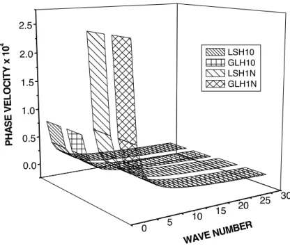
−2MATLAB software 7.04 has been used for numerical computation of the resulting quantities. The values of phase velocity and attenuation coefficient with wave number at the stress free boundary with thermally insulated and impermeable boundaries, isothermal and isoconcentrated boundaries alongwith the relaxation times are shown in fig.1 and fig.2. Normal stress, tangential stress, tan-gential couple stress, microstress, temperature change, and mass concentration with wave number has been determine at the surface
x
3
=
1
, and are shown in figs.3-8. In all figures, the words LSH10 and GLH10 symbolize the graphs of L-S and G-L theories in microstretch thermoelastic diffusion medium for the thermally insulated boundary and impermeable boundary and are represented by and respectively, while, the words LSH1N and GLH1N symbolize the graphs of L-S and G-L theories in microstretch thermoelastic diffusion medium for the isothermal boundary and isoconcentrated boundary and represented by and respectively.Phase Velocity
Figure 1 Variation of phase velocity w.r.t wave number
Attenuation
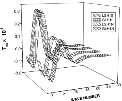
Fig.2 depicts the variation of attenuation with wave number ξ. The trend of variation and behav-ior of attenuation for LSH10 is opposite to LSH1N and GLH10 is opposite to GLH1N for 0≤ξ≤7, the values of attenuation for smaller values of wave number increase sharply for LSH10 and GLH10, while, decrease strictly for LSH1N and GLH1N which becomes dispersionless for higher values of ξ for all the cases. Fig.3 shows the variation of normal stress component T33 with wave number ξ. The behavior of T33 is oscillating for 0≤ξ≤12 and stable for 20≤ξ≤30 attaining max-imum at ξ=5 for all the cases while the corresponding values are different in magnitude. The val-ues of T33 are more in case of LSH10 and small for LSH1N, the similar behavior can be noticed for GLH10 and GLH1N respectively.
0.0 0.5 1.0 1.5 2.0 2.5
0 5
10 15
20 25 30 LSH10
GLH10 LSH1N GLH1N
P
H
A
S
E
V
E
L
O
C
IT
Y
x
1
0
4
WAVE N
Figure 2 Variation of attenuation w.r.t wave number
Figure 3 Variation of T33 w.r.t wave number
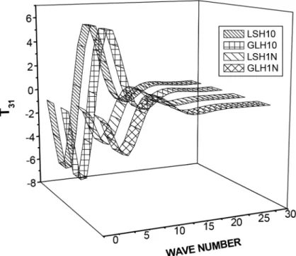
Fig.4 depicts the variation of tangential stress component T31 with wave number ξ. The trend of
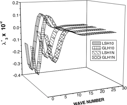
variation and behavior of T31 is similar to T33, but, the corresponding values are different in magni-tude. An appreciable difference due to various boundaries is noticed for the values of T31. Figs.5-6 exhibits the variations of couple stress components m
32 and microstress λ3 *
with wave number. The graph of m
32 and λ3 *
shows similar behavior, but their corresponding values are different in magni-tude. For the higher value of ξ, the values of and *
are convergent, after showing a respecta--0.4
-0.2 -0.0 0.2 0.4
0 5
10 15
20 25 30
LSH10 GLH10 LSH1N GLH1N
A
T
T
E
N
U
A
T
IO
N
x
1
0
4
WAVE NUM
BER
-0.2 -0.1 0.0 0.1 0.2 0.3
0 5
10 15
20 25
30
LSH10 GLH10 LSH1N GLH1N
T
33
!
1
0
-3
WAVE NUM
ble oscillation for smaller values of ξ. Adequate difference at ξ=7, in the values of m
32 is noticed corresponding to all the cases, while a major difference can be noticed due to the different bounda-ries.
Figure 4 Variation of T31 w.r.t wave number
Figure 5 Variation of m32 w.r.t wave number
-0.3 -0.2 -0.1 0.0 0.1 0.2 0.3 0.4
0 5
10 15
20 25
30
LSH10 GLH10 LSH1N GLH1N
m
3
2
x
1
0
-2
Figure 6 Variation of w.r.t wave number
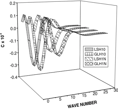
Fig.7 depicts the variation of concentration C with wave number ξ. The value of C first increase for 0≤ξ≤5, become oscillatory for 5<ξ≤15 and finally got dispersionless for 15<ξ≤30.
Concen-tration attains its minimum value for LSH10, while maximum value for LSH1N, at ξ=4. Similar
trend is noticed by GLH10 and LSH1N, however, corresponding values are different in magnitude.
Fig.8 exhibits the variation of temperature change T with wave number ξ. The graph indicates that the values T for LSH10 and GLH10 decreases monotonically for 0≤ξ≤6, increase smoothly for 6<ξ≤10 and becomes stable further, on the other hand, a good difference in the value of T can be noticed in cases of GLH10 when compared to GLH1N, for smaller value of wave number.
-0.4 -0.3 -0.2 -0.1 0.0 0.1 0.2
0 5
10 15 20
25 30 LSH10 GLH10 LSH1N GLH1N
h
3
x
1
0
-2
Figure 7 Variation of concentration ‘C’ w.r.t wave number
Figure 8 Variation of temperature ‘T’ w.r.t wave number
11 CONCLUSION
The propagation of Rayleigh waves in a homogeneous isotropic microstretch thermoelastic diffusion solid half-space subjected to stress-free, tangential couple stress, microstress , thermally
insulat--0.4 -0.3 -0.2 -0.1 0.0 0.1 0.2
0 5
10 15
20 25 30 LSH10 GLH10 LSH1N GLH1N
C
x
1
0
-3
WAVE NUMB ER
-0.07 -0.02 0.03 0.08 0.13 0.18 0.23 0.28 0.33
0 5
10 15
20 25 30 LSH10 GLH10 LSH1N GLH1N
T
x
1
0
3
WAVE NUM
ed/isothermal, and impermeable/isoconcentrated boundary conditions has been investigated. Secu-lar equations for surface wave propagation in the considered media are derived. Appreciable effects of relaxation times on the phase velocity, attenuation coefficient, normal stress, tangential stress, couple stress, microstress, temperature change, and mass concentration have been observed. It is observed that the trend of variation and behavior of the all derived components converges towards zero with the increase of wave number. It has also been noticed that the graphs of T
33,T31,m32,λ3 *
,C and T shows respectable oscillation for 0≤ξ≤15 and finally becomes dispersionless. The magnitude of components in all the graphs, except the phase velocity are more in case of thermally insulated and impermeable boundaries when compared to isothermal and isoconcentrated boundaries, respec-tively.
References
De, S.N. and Sen-Gupta, P. R.,(1974). Surface waves in micropolar elastic media., Bull. Acad. Pol. Sci. Ser. Sci. Technol. 22:137-146.
Dudziak W. and Kowalski S.J.,(1989).Theory of thermodiffusion for solids.,Int. J. Heat Mass Transfer. 32:2005-2013.
Eringen A.C., (1966).Mechanics of micromorphic materials., Proceedings of the II International Congress of Ap-plied Mechanics. H. Gortler (ed.), Springer, Berlin, 131–138.
Eringen A.C., (1966). Linear theory of micropolar elasticity, J. Math. Mech.15: 909–923.
Eringen A.C., (1968). Mechanics of micromorphic continua. Mechanics of Generalized Continua. E. Kroner (ed.), IUTAM Symposium, Freudenstadt-Stuttgart, Springer, Berlin, 18–35.
Eringen A.C., (1971). Micropolar elastic solids with stretch, Prof Dr Mustafa Inan Anisina, Ari Kitabevi Mat-baasi, Istanbul, 1–18
Eringen A.C., (1984). Plane wave in nonlocal micropolar elasticity, Int. J. Eng. Sci. 22:1113–1121.
Eringen A.C., (1990). Theory of thermo-microstretch elastic solids., Int. J. Eng. Sci. 28:1291–1301.
Eringen A.C., (1999). Microcontinuum Field Theories I: Foundations and Solids ,Springer-Verlag, New York. Iesan D. and Pompei A., (1995).On the equilibrium theory of microstretch elastic solids. Int. J. Eng. Sci. 33:399-410.
Kumar R. and Kansal T., (2008). Propagation of Lamb waves in transversely isotropic thermoelastic diffusive plate., Int. J. Sol. Struc. 45:5890-5913.
Kumar R. and Kansal T.,(2009).Propagation of Rayleigh waves in transversely isotropic generalized thermoelas-tic diffusion. J. Eng. Phy. Thermophysics. 82:1199-1210.
Kumar R.and Kansal T., (2011).Fundamental solution in the theory of thermomicrostretch elastic diffusive sol-ids, Int. Sch. Res. Net.,Article ID 764632, 15 pages.
Kumar R.and Partap G., (2009). Wave propagation in microstretch thermoelastic plate bordered with layers of inviscid liquid, Multidiscipline Modeling in Mat. Str. 5:171-184.
Nowacki W. (a)., (1974).Dynamical problems of thermodiffusion in solids-I, Bulletin of Polish Academy of Sci-ences Series, Science and Technology. 22: 55- 64.
Nowacki W. (c).,(1974). Dynamical problems of thermodiffusion in solids-III, Bulletin of Polish Academy of Sci-ences Series, Science and Technology 22:275- 276.
Nowacki W., (1976).Dynamical problems of diffusion in solids, Eng. Fract. Mech. 8:261-266.
Olesiak Z.S. and Pyryev Y.A., (1995). A coupled quasi-stationary problem of thermodiffusion for an elastic cylin-der, Int. J. Eng. Sci. 33:773-780.
Othman M.I.A. and Lotfy K.H., (2010). On the plane waves of generalized thermo-microstretch elastic half-space under three theories, Int. Comm. Heat Mass Transfer 37:192-200.
Quintanilla R., (2002). On the spatial decay for the dynamical problem of thermo-microstretch elastic solids, Int. J. Eng. Sci. 40:109–121.
Richter Ch. F., (1958). Elementary Seismology. W. H. Freeman and Company, San Francisco.
Sharma J. N., (2007). Generalized thermoelastic diffusive waves in heat conducting materials, J. Sound Vib. 301:979– 993.
Sharma J. N., Kumar S. and Sharma Y. D., (2008). Propagation of Rayleigh surface waves in microstretch thermoelastic continua under inviscid fluid loadings, J. Ther. Stress. 31:18-39.
Sharma J. N., Sharma Y. D. and Sharma P. K., (2008).On the propagation of elastothermodiffusive surface waves in heat conducting materials, J. Sound Vib.315:927–938.
Sherief H.H., Hamza F.A. and Saleh H.A., (2004). The theory of generalized thermoelastic diffusion, Int. J.Eng. Sci. 42:591-608.