A Novel Explicit-Implicit Coupled Solution Method of SWE for Long-term River Meandering Process Induced by Dambreak

Journal of Applied Fluid Mechanics, Vol. 9, No. 6, pp. 2647-2660, 2016. Available online at www.jafmonline.net, ISSN 1735-3572, EISSN 1735-3645.

A Novel Explicit-Implicit Coupled Solution Method of

SWE for Long-term River Meandering Process

Induced by Dambreak

X. G. Zheng

1

, J. H. Pu

2

, R. D. Chen

1†

, X. N. Liu

1

and S. D. Shao

1

1 _{State Key Laboratory of Hydraulics and Mountain River Engineering, Sichuan University, Chengdu,}

610065, China

2 _{School of Engineering, Faculty of Engineering and Informatics, University of Bradford, Bradford, BD7}

1DP, UK

†Corresponding Author Email: chenridong1984@163.com

(Received December 7, 2015; accepted April 18, 2016)

A

BSTRACT

Large amount of sediment deposits in the reservoir area can cause dam break, which not only leads to an immeasurable loss to the society, but also the sediments from the reservoir can be transported to generate further problems in the downstream catchment. This study aims to investigate the short-to-long term sediment transport and channel meandering process under such a situation. A coupled explicit-implicit technique based on the Euler-Lagrangian method (ELM) is used to solve the hydrodynamic equations, in which both the small and large time steps are used separately for the fluid and sediment marching. The main feature of the model is the use of the Characteristic-Based Split (CBS) method for the local time step iteration to correct the ELM traced lines. Based on the solved flow field, a standard Total Variation Diminishing (TVD) finite volume scheme is applied to solve the sediment transportation equation. The proposed model is first validated by a benchmark dambreak water flow experiment to validate the efficiency and accuracy of ELM modelling capability. Then an idealized engineering dambreak flow is used to investigate the long-term downstream channel meandering process with non-uniform sediment transport. The results showed that both the hydrodynamic and morphologic features have been well predicted by the proposed coupled model.

Keywords:SWE; Explicit-implicit coupled; Dam break; Eulerian-Lagrangian; River meandering.

1. I

NTRODUCTION

The flow and sediment transport after the dambreak demonstrate two distinct features: [1] short-distance flow effects on the immediate downstream location; and [2] long-distance flow influences on the wide downstream landscape through morphologic process. A qualified numerical model is thus required to address both the processes with different time steps so as to efficiently predict the long-term downstream river meandering process.

Present studies on such a meandering channel have not reached the mature stage, because of the complex nature of the morphological changes, and the difficulties in the model validation from very limited field observations. Besides, it is also quite difficult to scale the results of flume experiments to natural meandering channels. As a result, the relevant studies have been mainly conducted by the statistical analysis of historical data and numerical simulations, and the latter is becoming more

meandering processes have also been tentatively addressed: Ronco et al. (2009) used 1D model to study a 10-year morphological evolution of the Zambezi River. Furthermore, to investigate more detailed flow information in the cross-section, Yang and Jiang (2011) used a 2D Depth-Integrated Velocity and Solute Transport (DIVAST) model for the Yellow River Delta evolutions from 1992 to 1995. Even more complex 3D model has also been proposed by Kolahdoozan and Falconer (2003) for very long-term Humber Estuary morphological changes by using an Alternation Direction Implicit (ADI) finite difference algorithm. More recently good improvements in the SWE solution schemes have been reported by Pu et al. (2012; 2014). To further improve the prediction of dambreak flow from being transient to steady state, and to address the long-term morphological evolutions, the present study aims to propose a robust numerical model based on the Eulerian-Lagrangian (ELM) method to solve the hydrodynamic equations, during which the n+1 time step is tracked reversely along the streamline to the n time step, thus avoiding the conventional Euler number restriction imposed by the Courant stability criterion. The developed ELM method utilizes a coupled explicit-implicit numerical scheme with the use of both small and large time steps, hence fulfils the cross-scale flow computational requirement. In the model implementation, water levels and flow fields are calculated by the implicit approach and corrected explicitly by the Characteristic-Based Split (CBS) method at each local time step. After the flow field is obtained, the sediment equations are then solved by the TVD finite volume method. To demonstrate the model performance, both short-time flood flow and long-time channel meandering process induced by the dambreaks are used as the case study.

This work is motivated by the fact that the efficiency of most explicit numerical schemes is heavily constrained by the computational time step, especially for the complex topographies and physical boundaries, although it has the advantages of being straightforward in numerical algorithm and readily adaptable to GPU acceleration. On the other hand, the computational accuracy of implicit schemes is generally lower than that of the explicit ones, due to the use of significantly larger time step and other truncation errors, in spite of their good numerical efficiency and stability. For the study of long-term river and morphological process, the implicit solution method could have more promising potentials, as long as its accuracy can be built to a suitable level up to the explicit solution. Thus the present work aims to merge the merits of both and develop a coupled explicit-implicit solution scheme for practical engineering purpose.

2. S

HALLOW

W

ATER

E

QUATIONS

(SWE

S

)

M

ODEL WITH

S

EDIMENT

T

RANSPORT

In this work the SWEs model is used with the

sediment transport equations to investigate the long-term river morphological process. Eqs. (1) - (4) show the 2D SWEs water-sediment flow model (Chen et al., 2015).

0 ) (       u h t

 ₍₁₎

3 / 1 2 2 ) ( h gn gh h A dt h d H u u u

u _{    (2)}



S S



A h S

dt hS d H 2 * )

( _{    (3)}









s *

b S S

t z        

 qb

1 (4)

where _ = water surface; t = time; h = flow depth; u

 

u,v are the 2D flow velocities; n = bed roughness; g = gravitational acceleration; S = sediment suspended load concentration;  = sediment settling velocity; *

S = maximum suspended load carrying capacity;  = erosion-deposition coefficient (0.25 for the erosion-deposition, 1.0 for the erosion and 0.5 for the transition); z_b = movable bed layer thickness;



= bed porosity;

s



= density of sediment grain; and _{( )}

, by

bx b q q

q are the horizontal 2D sediment bedload transport (but not considered in present study, as we focus on the morphological process of plain rivers consisting of mainly fine sediment materials). The horizontal eddy viscosity coefficient

H

A in Eqs. (2) and (3) is represented as 5 . 0 2 2 2 5 . 0                                       y v y u x v x u A C

AH s

(5)

where C_s = Horcon coefficient, set 0.1 – 0.2 in this study; and A = node influence area.

Here we need to note that the sediment transport parameters in Eqs. (3) - (4) do not directly affect the source term of SWE Eqs. (1) - (2). This is based on the assumption that the sediment exchange between the water column and erodible bed is not dominant, so the flow structure has not been significantly modified by the existence of sediment mixture. This should be true for many plain rivers located in the low-sediment areas.

3.

N

UMERICAL

A

PPROACH

streamlines may not be accurately traceable by using the ELM traced lines since they are quite different after the transient flow process. To improve this tracking, an explicit Characteristic-based Splitting (CBS) method shall be used within each computational iteration to couple with the implicit algorithm and thus correct the solved water levels and velocity fields, aiming to recover the lost detailed flow information. Finally, we adopt a standard TVD finite volume scheme to solve the sediment transport equations

.

3.1 Implicit Eulerian-Lagrangian Method

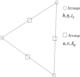
In an ELM computation, the spatially-discretized triangular meshes are used. The schematic diagram of the present ELM tracking nodes (i.e. by using the Moving Least Squares (MLS)), is shown in Fig. 1.

Fig. 1. Schematic illustration of ELM tracking.

As suggested by Zhang et al. (2004), the tracking of streamlines contributes to the core computational cost of the ELM method, so this efficiency is crucial to the modelling of the hydrodynamic system. To solve the continuity and momentum equations, the finite element method will be used after getting _u* _{from the ELM tracking, with the}

layout of the computational variables as being shown in Fig. 2.

Fig. 2. Layout of computational nodes and variables.

Thus the momentum equation can be written as below and solved by the following procedures:

























                              _    d N N d u Nh N d u Nh N t d u Nh N d u Nh N d u Nh N t d N N n T n n T n n n T n n T n n n T n n n T n T     1 1 2 1 1 1 1 2 1

(6)

where





4 5

3 2

1 I tI 1 tI tI

I     











 _{    }

 N N g t P N N d

I T n1 2 2 T n1

1   









 



       

_

_ d NU N t NQ N t N N I n T T n T    1 2



  _   2 2 1

3 t N NU d

I



T _nn









_

_ 

 t N NU d

I n n T  1 4



  _   1 1 1

5 t N NU d

I nn

T



When the node i belongs to the first type of boundary conditions, it will not be solved; whereas it belongs to the second type of the boundary conditions, then





4 3

2

1 I tI 1 tI

I     . In Eq. (6) N is the shape function, ₁ is the principle boundary,

2

 is the natural boundary, and

0

.

5







1

is the explicit-implicit weighting coefficient. So the next solution procedures are: [1] use the ELM method to calculate the velocity *

u at time n; [2] solve the continuity equation to obtain the water level at time

1



n

, n1_{; and [3] substitute it into the momentum}

equation and solve the velocity _un1_.

3.2 Explicit Galerkin Finite Element

Method

The Galerkin-FEM method is well-known for solving the self-adjoint problems with good consistency (Zienkiewicz and Taylor, 2006). Here it will be used with the CBS method to explicitly calculate _u* _{for the continuity and}

 

nn i i j j S x k x x U t                            

 

                          S x k x x U x U t i i j j k n k   2

2

₍₇₎

where i and j represent the x and y direction domains, respectively. For detailed solution procedures, refer to Chen et al. (2015).

To achieve a stable simulation, the computational time step should satisfy the following Courant criterion: u    c l C t em FL

(8)

where l_em = characteristic element size; c gh is the wave celerity; and

FL

C = Courant stability coefficient.

3.3 Coupled Explicit-Implicit Method

In the proposed coupled explicit-implicit solution method, the initial flow field is computed by the implicit approach and then it is corrected by using the explicit algorithm during each time step. A schematic illustration of the coupled method is shown in Fig. 3.

Fig. 3. Schematic illustration of coupled explicit-implicit computations.

Since the implicit computation is based on the streamline tracking, for the complex dambreak flows that involve both the transient and steady flow regimes, the actual and modelled traced lines can be quite different. Hence an explicit iterative solver has to be used amid time step n~n1 for the known flow field _un_、hn_、 n1

u 、hn1 by using the linear interpolation method. This could be computationally achieved by using the intermediate time m to obtain _um _and m

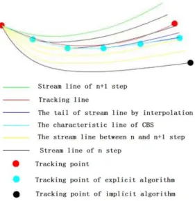
h . As the nodal information around n~n1 time step is known, the flow field at different nodes can be found explicitly within a local time step by using the nodal-based CBS explicit algorithm. The coupled solution process can also be schematically viewed in Fig. 4.

The CBS method uses the linearized characteristic lines as the traced lines, which is similar to the linear interpolation scheme used in the Smoothed Particle Hydrodynamics (SPH) method. For a reasonably small time step between n~n1, the gradient of the traced and stream lines can be

considered being identical. Thus the monotonic variation within a time step using CBS algorithm makes the traced and stream lines have a small deviation when the implicit scheme is used. After the flow field is found at time n1 by the implicit solution, the explicit method is used at the local time step within the correction phase to enhance the efficiency of iteration (compared to a fully implicit method). Also the benefit of this coupled method is that by simply increasing the amount of explicit computations, the information lost in the implicit computations, i.e. flow field, can be recovered or even restored

.

In terms of

FL

C number, the implicit scheme allows the use of a value 1 ~ 10 for the local time step under a weighted average scheme, while the explicit scheme only allows for 0.2 ~ 0.4, by taking into account the computational efficiency and accuracy. In order to maintain the consistency of the proposed model in the temporal flow field, the explicit iterations shall not advance in time but be bounded by the implicit ones.

Fig. 4. Schematic view of stream/trace lines in a coupled computation

3.4 Sediment Transport Computation

where









       



 



N

r S S h l u S S h l u j j j j j j j j j h l u j j h l u h l u i j j j j j i j j j j 0 0 0 2 2   







i j



j j j h l u i j j j j j S S h l u S S h l u

r jjj

  



0

After the tests, we found that among several commonly used slope limiters the Van Leer limiter shows the best result with the TVD scheme, as also suggested by Hu et al. (2006).

Key sediment parameters are also needed to solve the sediment transport equations. Since the sediment bedload transport is not the dominant factor in the proposed plain rivers, it is ignored in the morphological process and thus only the suspended load is considered. The sediment falling velocity is determined by using the following equation of Zhang (1961):

d . gd .

d

. s 

   

 1395 109 1395

2         



(10)

where  = kinematic viscosity of water; d = sediment size;and



_s and  = gravity density of the sediment grain and water, respectively. The suspended sediment carrying capacity of the flow can be calculated by

m gh U k S _        3

*

(11)

where k and m = empirical sediment coefficients, whose values depend on the particular river characteristics.

In order to address the non-uniformity of suspended load transport and the bed material adjustment arising from the alluvial deformation, some modifications of the above equations are also provided by Zhang (1998). For example, for the non-uniform sediment settling velocity, it has the following general form as:

 

 

 





                            _     mm d gd s mm d mm gd s d mm d gd s 1 1 1 . 1 1 1 . 0 1 1 01 . 0 1 10 1 . 0 1 18 1 5 . 0 5 . 0 2 3 2     (12) where

s

= density ratio between sediment grain and clear water.

Furthermore, the threshold grain size separating the bed load and suspended load materials can be determined by the so-called suspension index, which is represented by

*

u

Rz







(13)

where



= 0.41 is the Von Karmon constant; and

*

u = frictional velocity. From numerous field case studies, a general guideline is that Rz > 4.166 falls into the bed load and

Rz

< 4.166 falls into the suspended load. Meanwhile, the sediment non-uniformity should also be reflected in the transport Eq. (11) as well as the bed deformation Eq. (4), as detailed in Liu (2004) and Wu and Wang (2000).

3.5 Numerical Boundary Conditions

In terms of the boundary conditions, there are basically three types of the boundary as utilized in this model. They include: [1] open boundary, which is applied in the flow inlet and outlet; [2] land boundary, upon which a slip boundary is imposed; and [3] moving boundary, which is represented by the continuous changes of flow and sediment transport. More details on these can be found in Chen et al. (2015)

.

4. M

ODEL

V

ALIDATIONS AND

A

PPLICATIONS

In this section, two tests are carried out to validate and apply the model to practical engineering scenarios. In the first test, a fixed bed shallow dambreak flow is used to validate the coupled model accuracy and efficiency to reproduce the shock flood waves. The second test uses an idealized dambreak flow aiming to demonstrate the model capability to simulate long-term morphological process and sediment transport.

4.1 Fixed Bed Dambreak Flow Experiment

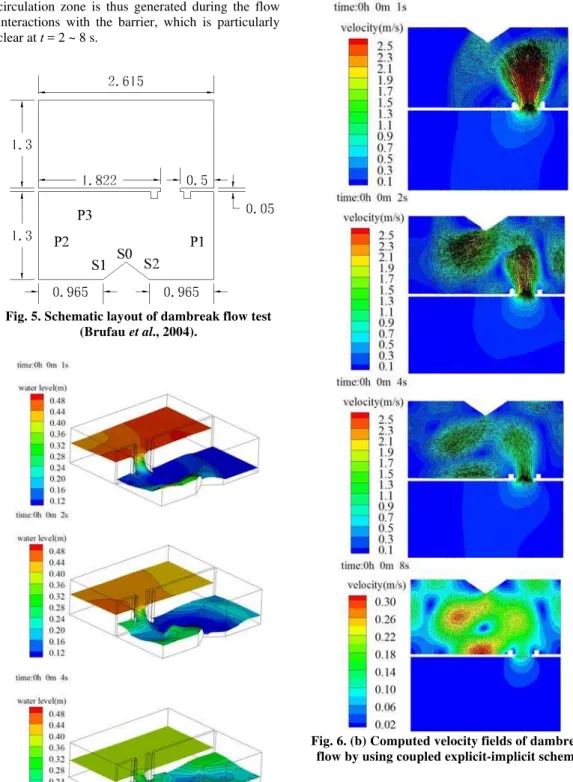
This test is based on the fixed bed dambreak flow experiment carried out by the CITEEC laboratory (Brufau et al., 2004). In the experiment, the flow areas were divided into two rectangular pools that were bounded by the solid walls and separated by a sluice gate. The water detained in the upstream tank had a high potential energy, and the downstream floodplain provided the outlet flooded area (after the dam breaks). A triangular barrier was installed on the downstream side of the wall (shown in Fig. 5). The bed roughness of whole computational domain was n = 0.018 following Brufau et al. (2004). The initial water depths on the upstream and downstream tanks were 0.5 m and 0.1 m, respectively. At the initial time t = 0, the sluice gate was opened instantaneously and completely to allow the flood water to propagate from the upstream to downstream tanks. A schematic layout of the experimental condition is shown in Fig. 5 with six measurement points.

circulation zone is thus generated during the flow interactions with the barrier, which is particularly clear at t = 2 ~ 8 s.

Fig. 5. Schematic layout of dambreak flow test (Brufau et al., 2004).

Fig. 6. (a) Computed water surfaces of dambreak flow by using coupled explicit-implicit scheme.

Fig. 6. (b) Computed velocity fields of dambreak flow by using coupled explicit-implicit scheme.

the lost flow information computed by the fully implicit scheme. Besides, since the explicit computation was actually carried out within the local time step, the coupled numerical scheme only increased the computational load by 20%.

Fig. 6. (c) Computed velocity fields of dambreak flow by using fully explicit scheme.

Fig. 6. (d) Computed velocity fields of dambreak flow by using fully implicit scheme.

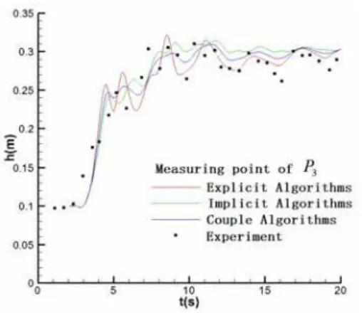
To further quantify the accuracy of model simulations, the computed water depths at six measurement points (shown as S0, S1, S2, and P1, P2,

P3 in Fig. 5) are presented in Fig. 7. To illustrate the

Fig. 7. Computed and measured water level variations of dambreak flow.

It shows that three models give generally satisfactory agreement with the measured data at all gauging locations. The fully explicit computations predicted much larger water level variations than the implicit ones, while the coupled computations predicted the water levels somewhere between the two. However, compared with the fully explicit and implicit models, the coupled model has no restriction in dealing with either the transient or steady flows, which is an important asset for the study of cross-scale flow problems in practical engineering field. Besides, the coupled model is also able to predict highly complex and unsteady flood flow propagations and its interactions with the triangular obstacle, and the precise location and amplitude of the shock waves are well captured. The errors could be attributed to the 3D experimental flows which were modelled by the 2D numerical schemes.

4.2

Long-Term

Channel

Meandering

Process

After dambreak the downstream river will be flooded by the incoming reservoir water and the eroded sediment materials, which could create very complex morphological scenarios and long-term river meandering patterns. Due to the large amount of momentum carried by the dambreak flow, the flooding waves could cause the failure of river dikes and further aggravate the sediment transport. When the sediment materials in a river reach a certain limit, the flow could diffuse these sediments to the downstream floodplain areas and thus develop the phenomenon of river channel meandering. In this section we will use the proposed coupled model to simulate this cross-scale flow and alluvial process.

Table 1 Compositions of initial sediment bed layer of downstream channel

Layer thickness from the top (m)

Sediment grain diameter (mm) Percentage of each sediment composition (%)

0.38 0.74 1.69 3.68 7.36 16.94

1 0.95 0.75 4.5 15.05 44.0 34.75

5 2.0 3.0 5.0 10.0 30.0 50.0

10 2.0 3.0 5.0 10.0 20.0 60.0

Table 2 Inflow sediment concentration of each composition

Sediment diameter (mm) 0.0038 0.0074 0.0169

Concentration (kg/m3_{) 3 3 13}

Sediment diameter (mm) 0.0368 0.0736 0.1694

Concentration (kg/m3_{) 5 4 2}

inflow sediment concentration is assumed to be 45 kg/m3_{. The composition of the initial sediment bed}

layer is summarized in Table 1 and the inflow sediment concentration for each of the composites is shown in Table 2. The sediment mixture is assumed to be non-uniform grains.

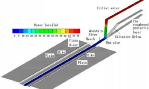
Besides, a reservoir is located on the most upstream side of the computational domain with an area of 15 km long and 0.7 km wide. Bed slope from the reservoir exit to the river channel is set as 0.6%, with the downstream floodplain being increased to 5 km in width on each side to accommodate the faster flow and sediment flushed from the dambreak water. A schematic view of the initial topography of the computational area is shown in Fig. 8.

Fig. 8. Schematic view of initial channel topography and reservoir area.

The initial water retained in the reservoir is 80 m in depth and the constant water depth in the downstream channel is 1.3 m. It is assumed that the downstream floodplain is dry at the beginning of the dambreak. The initial velocity of all the computational domains is set to be zero. The following computed results and analyses will be discussed in two different time scales, i.e. short period just after the dam break and long period up to the river meandering, so as to demonstrate the model capacity to study cross-scale flows.

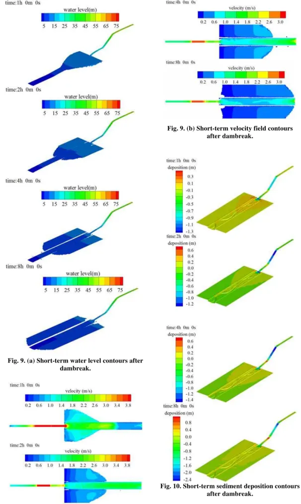
Fig. 9 (a) and (b) show the short period propagation of the dambreak flow at time t = 1, 2,

4 and 8 hours for the water depth and velocity field contours. It is shown that dambreak flooding is a rapidly transient disastrous process. After one hour of the dambreak, one can observe that the upper floodplain is quickly filled with about 2.5 m deep of water with the flood wave propagation being around 1 m/s in velocity. At t = 2 h, the separation of downstream and upstream flows is obvious as the supply of water from the upstream dam area reduced sharply. At later times after t = 4 h, the flows in the downstream main channel start to propagate more quickly and thus separate from the rest of flow in the floodplain area. After t = 8 h, the flows have reached the downstream boundary of the floodplain. As we can understand, even though the dambreak flow can create transient huge disaster due to the bore wave propagation in the downstream area, its effect on the morphological process is quite limited and this is only restricted within the upper section of the floodplain (within 8 hours). This is due to the fact that the dambreak flow propagates in the whole downstream area with the main flow energy being diverted. Although serious erosions and sedimentations can happen, they are mainly concentrated in the local areas near the dam site. The above analysis can be further supported by the corresponding sediment deposition maps as shown in Fig. 10. It implies that only long-term morphological process will cause the serious river meandering patterns. Nonetheless, the short-term simulations just after the dambreak suggest that the coupled numerical model is capable of capturing the short-term sediment transport in river flows.

Fig. 9. (a) Short-term water level contours after dambreak.

Fig. 9. (b) Short-term velocity field contours after dambreak.

Fig. 11. Sediment depositions (left) and flow velocity fields (right) at entrance of plain river.

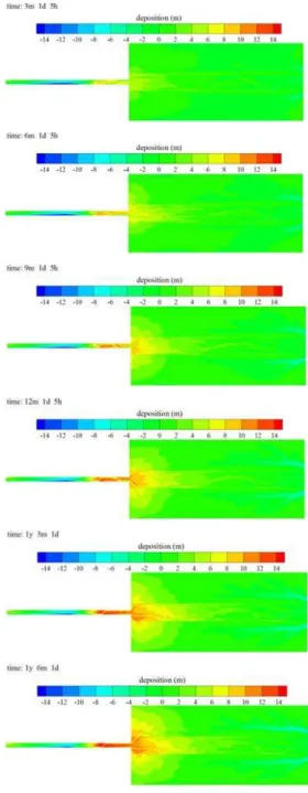
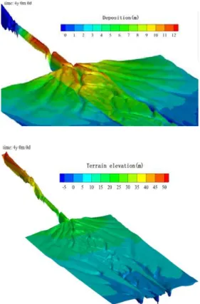
Fig. 12. Long-term downstream sediment deposition contours.

to 15 months). This is demonstrated by the fact that around 15-month time the deposition at the upper floodplain section has reached about 10 ~ 12 m in depth. This long-term sediment simulation has once again proved the coupled model’s capability due to its adoption of robust explicit-implicit numerical solution scheme for the cross-scale flows.

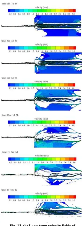
Fig. 13. (a) Long-term topographic evolutions of downstream meandering river.

Fig. 13. (b) Long-term velocity fields of downstream meandering river.

there could not exist a distinguished main channel and sidebank anymore, and the flow routes start to go random following the most prevailing bed configurations. As a result, the extent of river braiding could enlarge which causes further braiding in the main channel due to the significant modification of hydrodynamic and sediment conditions. Besides, the locations of meandering can also alternate in different directions of the channel arising from the complex and random water-sediment interactions.

Fig. 14. (a) Topography of very long-term (4 years) alluvial process and river meandering.

Fig. 14. (b) Velocity field of very long-term (3 years) alluvial process and river meandering.

Further evolutions of the topography and velocity field are provided in Fig. 14 (a) and (b), for the very long-term alluvial process and river meandering over several years in the time scale.

5. C

ONCLUSIONS

A coupled explicit-implicit numerical scheme has been proposed to simulate the cross-scale flow problems that involve short (transient) and long (steady state) time simulations. The numerical model was constructed by using a coupled FEM-FVM method to simulate the hydrodynamics and sediment transport. Reported laboratory dambreak flow experiments were used to validate the proposed flow model. The coupled simulations were also compared with the fully explicit and implicit numerical results. Then the model was used to study the long-term river morphological processes induced by an idealized dambreak, and it shows a good representation of both the short and long term river meandering patterns, which is due to the robustness of the coupled explicit and implicit schemes.

Future research work will be needed to quantitatively validate the long-term sediment/morphological simulations based on either the laboratory experiments or field observations. Besides, more critical evaluations of the relevant sediment transport equations and sediment parameters should be carried out.

A

CKNOWLEDGEMENTS

This research work is supported by Sichuan Science and Technology Support Plan (2014SZ0163), Start-up Grant for the Young Teachers of Sichuan University (2014SCU11056), and Open Research Fund of the State Key Laboratory of Hydraulics and Mountain River Engineering, Sichuan University (SKLH 1409; 1512).

R

EFERENCES

Bellos, C. and V. Hrissanthou (1998). Numerical simulation of sediment transport following a dam break. Water Resources Management 12, 397-407.

Bohorquez, P. and R. F. Feria (2008). Transport of suspended sediment under the dam-break flow on an inclined plane bed of arbitrary slope. Hydrol Process 22, 2615-2633.

Brufau, P., P. G. Navarro and M. E. V. Cendon (2004). Zero mass error using unsteady wetting-drying conditions in shallows over dry irregular topography. Int. J. Numer. Meth Fluids 45, 1047-1082.

Cao, Z. X., G. Pender, S. Wallis and P. Carling (2004). Computational dam-break hydraulics over erodible sediment bed. J. Hydraul. Eng. 130, 689-703.

Landslide dam failure and flood hydraulics, Part II: coupled mathematical modelling. Natural Hazards 59, 1021-1045.

Capart, H. and D. L. Young (1998). Formation of a jump by the dam-break wave over a granular bed. J. Fluid Mech. 372, 165-187.

Chen, R., S. Shao and X. Liu (2015). Water-sediment flow modelling for field case studies in Southwest China. Nat Haz 78, 1197-1224. Hu, K., C. G. Mingham and D. M. Causon (2006).

A mesh patching method for finite volume modelling of shallow water flow. Int. J. Num. Meth. Fluids 50(11), 1381-1404.

Kocaman, S. and H. O. Cagatay (2015). Investigation of dam-break induced shock waves impact on a vertical wall. J. Hydrol 525, 1-12.

Kolahdoozan, M. and R. A. Falconer (2003). Three-dimensional geo-morphological modelling of estuarine waters Int. J. Sediment Res 18, 1-16. Liu, X. N. (2004). Sand-Gravel Bed Load Transport

and Simulation. Ph. D. Thesis, Sichuan University, Chengdu, China (in Chinese). Ni, H., Z. Li. and H. Song (2010). Moving least

square curve and surface fitting with interpolation conditions. International Conference on Computer Application and System Modeling (ICCASM).

Pu, J. H., K. Hussain, S. D. Shao and Y. Huang (2014). Shallow sediment transport flow computation using time-varying sediment adaptation length. International Journal of Sediment Research 29(2), 171-183.

Pu, J. H., N. S. Cheng, S. K. Tan, S. D. Shao (2012). Source terms treatment of SWEs using surface gradient upwind method. J. Hydraul Res 50(2), 145-153.

Ronco, P., G. Fasolato and G. Disilvio (2009).

Modelling evolution of bed profile and grain size distribution in unsurveyed rivers. Int. J. Sediment Res. 24, 127-144.

Wang, Q., H. Zhang and J. Xia (2005). Meandering River Process and Modelling, Scientific Publishing, Beijing (in Chinese).

Wang, S. J., J. Ni and Q. Wang (2000). Research status and development trend of alluvial mechanics. Journal of Basic Science and Engineering 8(4), 362-369 (in Chinese). Wu, W. and S. Wang (2000). Nonuniform sediment

transport in fluvial rivers. J. Hydraul. Res. 38(6), 427-234.

Wu, W. and S. Y. Wang (2007). One-dimensional modeling of dam-break flow over movable beds. J. Hydraul. Eng. 133, 48-58.

Yang, C. and Jiang, C. B. (2011). A new model for predicting bed evolution in estuarine area and its application in Yellow River Delta. Journal of Hydrodynamics 23, 457-465.

Zech, Y., S. S. Frazao, B. Spinewine and N. Le Grelle (2008). Dam-break induced sediment movement: experimental approaches and numerical modelling. J. Hydraul. Res. 46(2), 176-190.

Zhang, R. J. (1961). Alluvial Dynamics, China Industry Publishing (in Chinese).

Zhang, R. J. (1998). Alluvial and Sediment Dynamics, Hydraulic and Hydroelectric Publishing, China (in Chinese).

Zhang, Y. L., A. M. Baptista and E. P. Myers (2004). A cross-scale model for 3D baroclinic circulation in estuary-plume-shelf systems: I. Formulation and skill assessment. Continental Shelf Res. 24, 2187-2214.