www.ann-geophys.net/28/1981/2010/ doi:10.5194/angeo-28-1981-2010
© Author(s) 2010. CC Attribution 3.0 License.
Annales
Geophysicae
A source location algorithm of lightning detection networks in China
Z. X. Hu, W. G. Zhao, and H. P. Zhu
School of Civil Engineering & Mechanics, Huazhong University of Science & Technology, Wuhan, China
Received: 3 July 2010 – Revised: 19 September 2010 – Accepted: 22 September 2010 – Published: 29 October 2010
Abstract. Fast and accurate retrieval of lightning sources is crucial to the early warning and quick repairs of lightning disaster. An algorithm for computing the location and onset time of cloud-to-ground lightning using the time-of-arrival (TOA) and azimuth-of-arrival (AOA) data is introduced in this paper. The algorithm can iteratively calculate the least-squares solution of a lightning source on an oblate spheroidal Earth. It contains a set of unique formulas to compute the geodesic distance and azimuth and an explicit method to compute the initial position using TOA data of only three sensors. Since the method accounts for the effects of the oblateness of the Earth, it would provide a more accurate solution than algorithms based on planar or spherical surface models. Numerical simulations are presented to test this al-gorithm and evaluate the performance of a lightning detec-tion network in the Hubei province of China. Since 1990s, the proposed algorithm has been used in many regional light-ning detection networks installed by the electric power sys-tem in China. It is expected that the proposed algorithm be used in more lightning detection networks and other location systems.
Keywords. Meteorology and atmospheric dynamics (Light-ning)
1 Introduction
Cloud-to-Ground (CG) lightning is one of the most dan-gerous atmospheric phenomena, often causing injuries and deaths, power system interruptions and equipment damage. Ground-based lightning detection networks have been in-stalled all over the world to provide useful information for CG lightning monitoring and research. Some providers are
Correspondence to:Z. X. Hu ([email protected])
the US National Lightning Detection Network (NLDN), the lightning detection network in Europe (LINET), Zeus in Eu-rope and Africa, and the World Wide Lightning Location net-work (WWLLN) (Cummins et al., 1998a; Betz et al., 2009; Chronis and Anagnostou, 2006; Dowden et al., 2008; Rodger et al., 2005, 2006), etc. These long-range lightning detec-tion networks primarily locate cloud-to-ground (CG) light-ning which is hazardous to human society. The data provided by these networks are widely used in electric power systems and for the aviation industry and meteorology research.
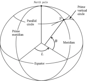
Fig. 1.The oblate spheroidal Earth geometry.Bis geodetic latitude, Lis longitude of a pointP on the oblate spheroidal Earth surface.
accuracy from combined technology (IMPACT) was devel-oped for lightning locations detected by NLDN (Cummins et al., 1998b). The IMPACT algorithm determines the best estimate of the lightning location by iteratively moving the stroke position along the surface of an oblate spheroidal Earth. Although the IMPACT algorithm is commercially successful, the specific software is proprietary and not widely distributed free of charge to the scientific community, and its data processing ability is constrained by computer power. In WWLLN, the lightning strokes are located using the “down-hill simplex” method (Dowden et al., 2008; John and Mead, 1965), which is also a searching method similar to the IM-PACT algorithm.
In this paper, an efficient CG lightning location algorithm is presented utilizing both TOA and AOA data. This algo-rithm has the advantages of retrieval lightning location and of onset time directly on the oblate spheroidal Earth surface. The earlier version of this algorithm was developed by Zhao et al. (1999), and since then it has been widely used in many regional lightning detection networks installed by the electric power system in China. Because of the demand for lightning monitoring for the space launch center in Wenchang, Hainan, we plan to install several lightning sensors in this region be-fore 2012. For this purpose, we have improved Zhao’s algo-rithm and are evaluating it in the present study. Compared to the earlier version of this algorithm, the explicit initial po-sition calculating method is more accurate after applying a simple unit circle model for choosing the best combination of three sensors. Furthermore, in the present version of the al-gorithm, a high accuracy expression of the geodesic distance calculating method is used, which enables this algorithm to
be employed for broader lightning detection networks. And for the first time, the algorithm is tested using a series of numerical simulations. In the ensuing section, the mathe-matical theory of lightning location on an oblate spheroidal Earth surface is introduced, as well as a unique method to compute the geodesic distance and azimuth. In Sect. 3, an explicit method for calculating an initial position of lightning source position using time of arrival measurements measured by three sensors is presented, and then the least-square posi-tion is computed iteratively. The performance of the pro-posed algorithm is tested in Sect. 4. Then, conclusions are drawn in Sect. 5.
2 CG lightning location principle
As shown in Fig. 1, the 1984 World Geodetic System Earth Ellipsoid (WGS-84) is used in our work: B = geodetic latitude and L=longitude. The curvature ra-dius at the poles C0=6399593.626 m, the first eccentric-ity e2=0.00669437992 and the second eccentricity e′2= 0.006739496745. The lightning source and the sensors are assumed to be located on the Earth surface; altitude is not considered in this paper.
Consider that the position of a CG lightning is(B,L)and its onset time ist. The TOA recorded by thei-th sensor is denoted asti,i=1, 2,···,n, and the AOA asαi, the arrival
time and azimuth equations can be written as ti=t+
SiP
c +εT i, (1) αi=βiP+εAi, (2)
where c is the speed of light in air, SiP and βiP are the
geodesic distance and azimuth between sensor i and the lightning source,εT i andεAiare the measurement errors of
arrival time and azimuth, respectively. The measurement er-rors are due to the effects of the nondeterministic nature of the lightning signals (Thomas et al., 2004), the propagation over complex terrain (Cummins et al., 1998a; Schulz and Diendorfer, 2000) and the clock error, and the reflexion of the signal will cause systematic error of AOA measurement (Orville, 1991). We compile all these effects into Gaussian error models, i.e., the errors are normally distributed with zero mean values and predefined variances which is denoted asσT2andσA2in this paper.
An efficient method for computing the geodesic distance and azimuth is given below, with which one can calculate the geodesic distance and azimuth with high accuracy. These formulas were first derived by Zhao (1997) for ellipsoidal geodesy research. As shown in Fig. 2, let (Bi,Li)denote
position of the i-th sensor, then the geodesic distance SiP
and azimuthβiP can be calculated by
(Bi+ϕi)=arctan
(1−e2)tanBP+e2
NisinBi
NPcosBP
Fig. 2. The geodesic pathSiP and the azimuthβiP andβP i
be-tween thei-th sensor and the lightning source position. P is the lightning location.
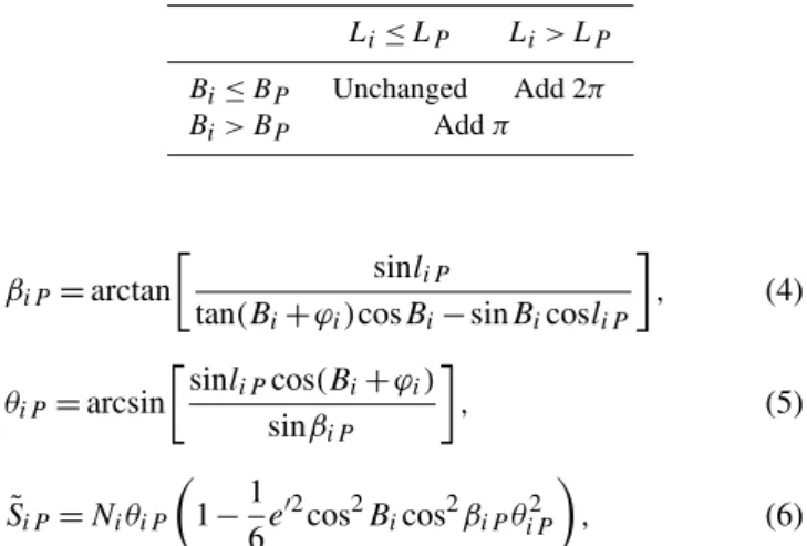
Table 1. Adjustment of the calculated value of the geodesic az-imuth.
Li≤LP Li> LP
Bi≤BP Unchanged Add 2π
Bi> BP Addπ
βiP=arctan
sinliP
tan(Bi+ϕi)cosBi−sinBicosliP
, (4)
θiP =arcsin
sinliPcos(Bi+ϕi)
sinβiP
, (5)
˜
SiP=NiθiP
1−1
6e ′2
cos2Bicos2βiPθiP2
, (6) whereliP =L−Li is the longitude difference between the
two points,ϕi is a correctional angle,θiP is radian measure
distance and Ni=
C0 p
1+e′2cos2B
i
(7) is the radius of curvature in prime vertical at the i-th sen-sor position. Equations (3) to (5) are closed formulas de-rived from the properties of the spherical surface; Eq. (6) is truncated forms from an infinite series that approaches the geodesic distance. Since the value of geodesic azimuth cal-culated by Eq. (4) lies in the range [−π2,
π
2] rather than the expected range [0, π], the calculated value should be ad-justed, as listed in Table 1. If the azimuth is very close to
π
2 or 3π
2 which corresponds to an unstable (extremely large) tangent value, the azimuth should be carefully determined to eliminate calculation error. In these two cases, the azimuth is close toπ2 whenLi< LP or close to 32π whenLi> LP.
An exchange of the subscript of Eq. (3)∼(6) can give (BP+ϕP),βP i,θP iandS˜P i. The values ofS˜iP are found to
Fig. 3. The geometry of CG lightning source retrieval using only three sensors #1, #2 and #3. P is the unknown lightning location; βdenotes azimuth;Sandθrepresent geodesic distance and radian measure distance, respectively.
coincide favorably with the centimeter accuracy ofS˜P i. The
geodesic distance is finally given by
SiP=
˜
SiP+ ˜SP i
2 . (8)
When SiP is shorter than 500 km, the calculation errors
of geodesic distance and azimuth are below 0.05 m and 0.01 arc sec, which is accurate enough for lightning detec-tion networks. For longer geodesic lines, we will verify this method by the results of a set of higher accuracy forms and compare it with Sodano’s forms (Sodano, 1965) in Sect. 4; the latter has been used by Koshak et al. for the lightning source location. Koshak et al. has proven that one can use Sodano’s forms to calculate geodetic distance within cen-timeter accuracy. The detailed derived process of the pro-posed forms Eq. (3)∼(6) is beyond the scope of this paper, for further details, the reader is referred to Zhao (1997).
3 CG lightning source retrieval algorithm
3.1 Explicit initial values
Time-of-arrival geolocation techniques were primarily devel-oped for marine navigation systems like the Loran system. Razin had derived an explicit position calculation method for the Loran system (Razin, 1967). The position calcula-tion method that we present here is similar but not identical to Razin’s explicit solution. Our method is simpler than Razin’s method and no osculating sphere (best-fit sphere) approach is needed for the approximation of the Earth’s surface sur-face. This method can provide initial CG lightning position and onset time for the subsequent Newton iteration algorithm which will give an improved solution.
Consider that recorded data of sensor 1, 2 and 3 are used to calculate the lightning location and onset time, as shown in Fig. 3. S12, β12, S13, and S13 can be calculated using Eq. (3)∼(8). Letθijdenote the radian measure distance from
pointitoj, which can be estimated by θij=
Sij
¯
R , (9)
hereR¯is the mean radius of curvature of the network com-posed of sensor 1, 2 and 3,
¯
R= C0
1+e′2cos2B¯, B¯=
B1+B2+B3
3 . (10)
According to the properties of arc lengths on a sphere, the spherical law of cosines can be written as
cosθ2P=cosθ12cosθ1P+sinθ12sinθ1Pcosφ1
cosθ3P=cosθ13cosθ1P+sinθ13sinθ1Pcosφ2, (11) whereφ1=β1P−β12 andφ2=β1P−β13. Let1ij denote
the radian measure range difference of a pair of sensors to the location of the lightning source, defined by
1ij=
Sj P−SiP
¯
R =
c(tj−ti)
¯
R . (12)
Now
θ2P=θ1P+112, θ3P=θ1P+113. (13) Substituting Eq. (13) into Eq. (11) yields two equations inθ1P andβ1P which, after transposition and division by
sinθ1P, become
(cos112−cosθ12)cotθ1P=sin112+sinθ12cosφ1 (cos113−cosθ13)cotθ1P=sin113+sinθ13cosφ2. (14) Note thatφ1 andφ2 can be expressed byβ1P. A forward
elimination of cotθ1P gives a standard trigonometric
equa-tion below:
A′sinβ1P+B′cosβ1P=C′, (15)
where
A′= −(sinθ12sinβ12−ksinθ13sinβ13) B′=sinθ12cosβ12−ksinθ13cosβ13 C′=ksin113−sin112
,
and
k=cos112−cosθ12 cos113−cosθ13 .
From Eq. (15), an initial value of the azimuth of the geodesic from lightning source position to sensor 1 can be obtained, given by
β10P = −arcsin(CA′′cosγ )−γ
= −arcsin(CB′′sinγ )−γ ,
(16) where
γ=arctan B′
A′
.
Note that β10P has two candidate values, one given by Eq. (16) (which should be plus 2πif it is negative), one given by subtracting the value of Eq. (16) fromπ. When four or more sensors’ data are available, there are many combina-tions for calculating of the initial azimuths of arrival of a cho-sen cho-sensor #1. Although each combination gives two candi-date values ofβ10P, the difference between all truth-values is very small. Thus the false-values can be eliminated. If only three sensors are trigged by the lightning signal, the false-values can be eliminated using azimuth-of-arrival measure-ment information. In some extreme cases, both of the calcu-lated values ofβ10P are used in the subsequent computation and both the two final solutions are recorded.
Hence the initial valueβ10P is obtained; the initial value of geodesic distance from the lightning source position to the selected sensor #1 can be calculated by
S10P= ¯Rθ10P, (17) whereθ10P can be calculated from any one of the equations in Eq. (14).
Finally, considering the property of spherical triangles, the initial values of lightning source position and onset time can be calculated by
B0P =arcsin(sinB1cosθ10P+cosB1sinθ10Pcosβ10P) L0P =L1+arcsin(sinθ10Psinβ10PsecBP0)
tP0 =t1−S10P/c
. (18)
3.2 Least square solution
right-hand side of Eqs. (1) and (2) in a Taylor series and keep-ing only terms below second order.
Denote the errors of the initial values provided by the explicit method above asδB=B−BP0, δL=L−L0P and δt=t−tP0. The approximate set of equations can be written as
cti≈ctP0+SiP0 +∂BSiPδB+∂LSiPδL+cδt, (19)
αi≈βiP0 +∂BβiPδB+∂LβiPδL, (20)
wherei=1,2,···,n, and the notations∂ωSiP and∂ωβiP are
the partial derivatives of the geodesic distance and azimuth toω, respectively, withω=B,L. All of these derivatives are evaluated at (BP0,L0P). Secant-type approximations of the derivatives may be used (Kohsak and Blakeslee, 2001), but we have derived exact representations for these derivatives, ∂BSiP=MP0cosβP i, (21)
∂LSiP=NP0cosBP0sinβP i, (22)
∂BβiP =MP0sinβP i/SiP0 , (23)
∂LβiP=NP0cosBP0cosβP i/SiP0 , (24)
whereNP0 is the radius of curvature in prime vertical at the initial lightning source location, calculated by Eq. (7), thus NP0cosBP0 is the radius of curvature of the parallel circle; andMP0 is the radius of curvature in meridian,
MP0= C0 (1+e′2cos2B0
P)3/2
(25) The equations defined by Eqs. (19) and (20) can be rewritten as an equation system form=2nrow measurements:
∂BS1P ∂LS1P c
∂BS2P ∂LS2P c
..
. ... ... ∂BSnP ∂LSnP c
∂Bβ1P ∂Lβ1P 0
∂Bβ2P ∂Lβ2P 0
..
. ... ... ∂BβnP ∂LβnP 0
δB δL δt =
c(t1−tP0)−S10P c(t2−tP0)−S20P
.. . c(tn−tP0)−SnP0
α1−β10P α2−β20P
.. . αn−βnP0
. (26)
Denote the coefficient matrix asA, the unknown vector asx
and column vector on the right-hand side asy, Eq. (26) can
be expressed as
Ax=y. (27)
This is an overdetermined linear system and the least square solution can be given by
ˆ
x=(ATW−1A)−1ATW−1y, (28)
whereWis the covariance matrix of the vector denoted by
y,
W=diag[c2σT2,···,c2σT2,σA2,···,σA2]2n×2n (29)
ThereforeW−1 is regarded as a matrix of weighting coef-ficients. In practical applications, the matrix W−1 can be replaced by
W−1=diag[1,···,1,c2σT2/σA2,···,c2σT2/σA2]2n×2n (30)
assuming that the variances of time-of-arrival measurements areσT =1 µs, and variances of azimuth-of-arrival
measure-ments areσA=π/180 rad.
Finally, an updated solution for the lightning source loca-tion and onset time can be given by
B=BP0+δB L=L0P+δL t =tP0+δt
. (31)
This updated solution can also be used as new initial values for a second iteration, but usually the results offered by only one or two iterations are good enough.
3.3 Retrieval errors
LetPdenote the covariance matrix ofxˆ. According to the statistical theory of the passive location (Torrieri, 1984), we obtain
P=(ATW−1A)−1, (32)
hereWis the covariance matrix defined by Eq. (29). It is also the covariance matrix of vector[B,L,t]T, and can be
rewritten as
P=
σB2 σBLσBt
σBL σL2 σLt
σBt σLt σt2
. (33)
The diagonal elements ofPcan give the variances of the er-rors of lightning positions and on set time, and the error el-lipses of the estimated location of lightning sources can be inferred by
P′=
MP2σB2 MPNPcosBPσBL
MPNPcosBPσBL NP2cos2BPσL2
, (34) whereMPandNPare the radius of curvature in meridian and
prime vertical at the estimated lightning source location, re-spectively. Lengths of semi-major axis and semi-minor axis are given by the eigenvalues of the matrixP′. The root mean square error (RMSE) of the source location estimator is RMSE=
q
NP2cos2B
PσL2+MP2σB2. (35)
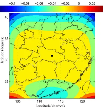
Fig. 4.The spatial distribution of the geodesic distance calculating difference between Eqs. (6) and (36) (in meter). The square is the beginning of each geodesic line. The difference is below in a large (yellow) area.
and uncertainty of time measurement, it’s easy to find that the source location accuracy (retrieval error) is dependent on the azimuths of the geodesic line from the lightning source location to each sensor, i.e.,βP i. We have investigated how
different combinations of the azimuthsβP iwill influence the
source location accuracy. If all the azimuths are concen-trated, say max(βP i)−min(βP i) <30◦, this corresponds to
the situation that the lightning source is outside and far away from the network, thus the retrieval error is very large. If the azimuths are dispersive, this corresponds to the situation that the source is inside or near the network, thus the retrieval error is small. This fact can be used to explain why the neces-sity of “surroundedness” for adequate accuracy applies to all lightning location networks that use timing alone for location (Dowden et al., 2008).
4 Algorithm performance
In this section, simulation results are presented to test and verify the above algorithm. Because the Hainan lightning detection network is under installation, we chose the Hubei lightning detection network as our test object. The network was installed in 1998 and is operated by the electric power system. This network contains 9 lightning detection sen-sors. The longitudes of these sensors range from 110◦E to 115◦E, and latitudes range from 29◦N to 33◦N, which will be shown in later figures. First, the geodesic distance and azimuth calculation methods are verified, then the accuracy
of the proposed explicit method for determining the initial position is investigated, and finally we present the estimated accuracy of a regional network (Hubei) under the assump-tion that all sensors participate in the calculaassump-tion of lightning sources’ positions. The computer generated time-of-arrival and azimuth-of-arrival measurements are given by a high ac-curacy expression (given later), and the retrieval algorithm uses the simplified geodesic distance and azimuth calculation forms Eq. (3)∼(6). We have examined the algorithm under two retrieval scenarios: location with random measurement errors and error free. The former is used to evaluate the spa-tial distribution of the location accuracy of the network and the latter is used to show the best performance of the pro-posed algorithm.
4.1 Verification of the geodesic distance and azimuth calculations
In order to verify the accuracy of the geodesic distance and azimuth calculation, results of a high accuracy version of forms derived by Zhao (1997) are used as references. This high accuracy version of forms is obtained by replacing Eq. (6) with
˜
SiP =NiθiP{1−
1 6η
2
iψiP2 [1−ηi2ψiP2 −ηi4(1−4sin2Bi)]θiP2
+1
8η 2
itanBiψiP(1−2η2iψiP2 −
1 6θ
2
iP)θiP3
− 1
120η 2
i[3tan
2B
i−4ψiP2 −7η
2
iψ
2
iP(3tan
2B
i−ψiP2 )]θ
4
iP
+ηi2( 1 335tan
2B
i−
1 315ψ
2
iP)θiP6 }, (36)
where ηi2 denotes e′2cos2Bi, and ψiP denotes cosβiP for
brevity. Compared to Eq. (6), this expression retains many high order terms, thus the geodesic distance can be estimated more accurately. It is worth noting that the geodesic azimuths calculated by both methods are identical because only Eq. (6) is changed. Their differences, geodesic distances calculated by Eq. (36) minus those calculated by Eq. (6), are shown in Fig. 4. The data are obtained by assuming that the lightning source locations are defined on a grid with (113◦E, 31◦N) as its center and a grid resolution of 0.2◦and assuming a light-ning detection sensor is located at the center of the grid. It can be inferred that the differences are less than 0.1 m in a large area. Given that the uncertainty of the time measure-ment of a lightning sensor is about 1 µs, corresponding to a ranging errorcεT≈300 m, the geodesic distance calculation
is accurate enough for the total investigated area. But we rec-ommend the high accuracy expression (36), yet noniterative, to be used in a broader lightning detection network such as WWLLN.
Fig. 5. Same as in Fig. 4 except for the geodesic distance differ-ence between the results obtained by Eq. (36) and forms derived by Sodano (in meter). There difference is below 1 cm in a large (blue) area.
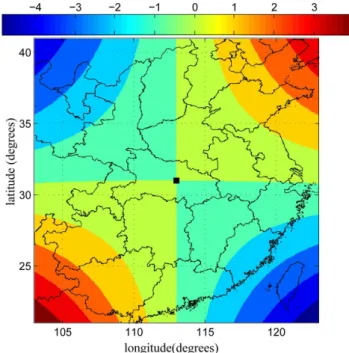
(Koshak and Blakeslee, 2001, Appendix) and asserted that one can calculate the geodesic distance using Sodano’s forms with centimeter accuracy. We have also compared Sodano’s solution to our high accuracy expression (36), and the results are shown in Figs. 5 and 6. Note that the discrepancies be-tween the two methods are trivial for most of the investigated area. The difference of the geodesic distance calculated by the two methods is below several centimeters all over the in-vestigated area. And the difference of the geodesic azimuth is below several arc sec, as shown in Fig. 6. Therefore, it is plausible that the geodesic distance and azimuth calculating method are accurate enough for lightning location applica-tion. For more discussion of the geodesic distance and az-imuth calculation, the reader is referred to Rapp (1993).
4.2 Error of the initial value
It is important to know how accurately the initial position and time can be calculated by the explicit method proposed in the above section. An initial position close to the true source’s position is essential for the next least square solution. Be-cause of the oblateness of the Earth, the spherical law of cosines (Eq. 11) represents an approximate relationship of the variables; thus the explicit initial position must contain some error. The other factors causing the initial position to depart from the true source’s position are the random timing errors. Figure 7 is the spatial distribution of the mean dis-tances from the calculated initial position to the true source’s location. The black square is the sites of three selected
sen-Fig. 6.Same as in Fig. 4 except for the geodesic azimuth difference (in arc sec). At the four corner of the map, the azimuth difference becomes large. Consider that the investigated map covers a large area, the azimuth calculating is accuracy enough for lightning loca-tion.
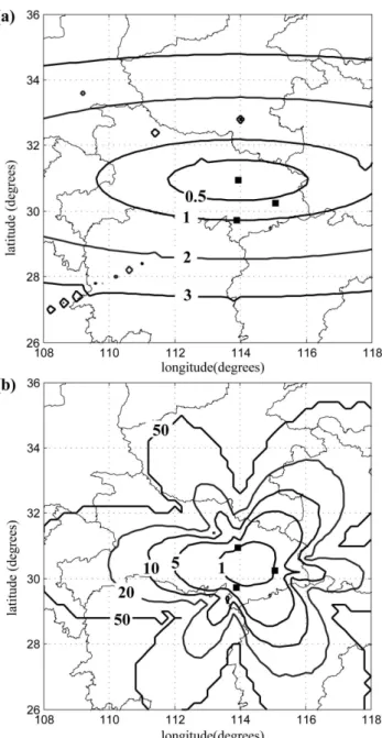
sors and the upper sensor is used as sensor #1. This small network is a part of the Hubei lightning detection network. The data are obtained by calculating 500 times the initial po-sition of the fictitious lightning sources on a grid with reso-lution of 0.2◦, and then the mean distance is computed as the error of the initial position. For each of the 500 trials, an ar-rival time error selected from a uniform random distribution (ranging from−√3 µs to√3 µs for Fig. 7b, but error free for Fig. 7a) is added. The elliptical area that gradually becomes large (error increasing from several tens of meters to several kilometers) in Fig. 7a is due to the effect of the oblateness of the Earth surface. Thus the sensor which receives the light-ning signal first (has the earliest time of arrival) should be regarded as sensor #1. It can be inferred from Fig. 7b that an initial position of the lightning source can be calculated with error below several kilometers when the source is not along the outer sensor baseline or far away from the network. And the largest error occurs in Fig. 7b when the lightning source is along the outer sensor baseline, which is caused by the timing error and amplified by the fact that the source is not surrounded by the sensors.
Fig. 7.Spatial distribution of mean distance from the calculated ini-tial position to the true source’s position (in kilometers), the upper sensor is used as sensor #1.(a)No random timing error is added to each sensor;(b)An arrival time error is added to each sensor, this error follows uniform random distribution (ranging from−√3 µs to √
3 µs).
line from the lightning source to each sensor should have the maximal range, i.e., disperse to the greatest extent. We have derived a simple model for choosing the best combination. As shown in Fig. 8, each azimuth defines a unit vector di-rected from the source to the sensor position, and a triangle is defined by the ends of the three vectors. Each combination is considered using this model and the best one is chosen if the corresponding triangle has the largest area. It should be noted that although the exact source location is unknown at
Fig. 8. The simple unit circle model for choosing the best combi-nation of three sensors. P is the lightning location, andβdenotes azimuth. Number 1, 2, and 3 is the projection of sensor #1, #2, and #3 on the unit circle, respectively.
the beginning, any proper initial position can be used as a replacement.
4.3 Network location accuracy
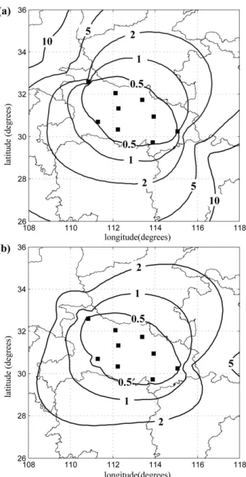
The accuracy of the initial values is degraded because of the Earth oblateness and the discarding of useful measurements (only three sensors’ time-of-arrival data are used). Thus the least square iterations can give updated solutions over the initial values. Figure 9 is the improved accuracy of the least square solutions when no measurement error is added into the computer generated data. The retrieval error is below one meter in most of the investigated area, which proves the excellent precision of the proposed algorithm. And Fig. 10 is the accuracy distribution when random measurement error (time error is the same as Fig. 7b, and azimuth measurement error is range from−√3 degree to√3 degree) is added. In Fig. 9 and Fig. 10a, only the time of arrival measurement is used for the lightning source retrieval. But in Fig. 10b, both TOA and AOA measurements are used in the calculation. A comparison of Fig. 10a and Fig. 10b shows the improvement of the accuracy after the fusion of AOA information, which is remarkable over the two “heads” of the network where the retrieval error in Fig. 10a is very large. But the improvement is not so obvious elsewhere when the source can be located with a small error.
Fig. 9.The spatial distribution of the improved accuracy of the least square positions when the measurements are error free (in meter). The lightning location error is below 10 m in the majority area of the investigated region.
than the simulated results. The coarse lines in Fig. 10 may be due to numerical error or nonrandomized characteristics of the computer generated data. All of the simulations have shown that the lightning location error is small in the periph-ery of the network (below 1000 m) and increases when the source is outside the network, especially along the outer sen-sor baseline. Thus the lightning location accuracy is affected by not only the measurements’ accuracy, but also by the rel-ative position between the source and the sensors.
5 Conclusions
An efficient algorithm for CG lightning source location is presented in this paper. This algorithm has been used in many regional lightning detection networks in China. We have ver-ified the geodesic distance and azimuth calculation method, which is an important part of the proposed algorithm. And the explicit initial position calculation method is evaluated by computer generated data. A simple unit circle model is used to select the best combination of three sensors for calculating the best initial position. In addition, the least square solution is tested using the Hubei lightning detection network. All of the simulations are performed using computer generated data, with or without measurement errors. When measure-ment errors do not exist, the lightning source retrieval error is only affected by the error of the geodesic distance and az-imuth calculation, therefore the retrieval error is favorably small. This is because the proposed algorithm has accounted
Fig. 10. Same as Fig. 7, except for the improved accuracy of the least square positions (in kilometer): (a)lightning source location using TOA measurement only,(b)lightning source location using both TOA and AOA measurements.
for the effects of the oblateness of the Earth. When random measurement errors are added to the simulations, a spatial distribution of the lightning source location accuracy is plot-ted. In the future, the location accuracy of lightning events reported by this network can be evaluated by the presented simulated contour map. Also, the location accuracy may be rapidly evaluated by the covariance matrix presented in Sect. 3.
Fig. 11. Spatial distribution of the lightning source location error (RMSE) given by Eq. (35), (in kilometer):(a)only TOA measure-ments are used,(b)both TOA and AOA measurements are used.
measurements will make the proposed algorithm more attrac-tive. Finally, we hope the proposed algorithm, along with the high accuracy expression for geodesic distance calculation, can be used for global lightning detection networks, such as Zeus and WWLLN, et al.
Acknowledgements. This work is supported by the National Key Technology R&D Program under Grant no. 2008BAC36B00.
Topical Editor P. Drobinski thanks Y. Zhang and another anony-mous referee for their help in evaluating this paper.
References
Betz, H. D., Schmidt, K., Laroche, P., Blanchet, P., Oettinger, W. P., Defer, E., Dziewit, Z., and Konarski, J.: LINET-An international lightning detection network in Europe, Atmos. Res., 91, 564– 573, 2009.
Chan, Y. T. and Ho, K. C.: A simple and efficient estimator for hyperbolic location, IEEE Transactions on Aerospace and Elec-tronic System, 42(8), 1905–1915, 1994.
Chronis, T. G. and Anagnostou, N.: Evaluation of a long-range lightning detection network with receivers in Europe and Africa. IEEE Transansactions on Geoscience and Remote Sensing, 44(6), 1504–1510, 2006.
Cummins, K. L., Krider, E. P., and Malone, M. D.: The U.S. National Lightning Detection Network and application of cloud-to-ground lightning data by electric power utilities, IEEE Transansactions on Electromagnetic Compatibility, 40(4), 465– 480, 1998a.
Cummins, K. L., Murphy, M. J., Bardo, E. A., Hiscox, W. L., Pyle, R. B., and Pifer, A. E.: A combined TOA/MDF technology up-grade of the U.S. National Lightning Detection Network, J. Geo-phys. Res., 103, 9035–9044, 1998b.
Cummins, K. L. and Murphy, M. J.: An overview of lightning locat-ing systems: history, techniques, and data uses, with an in-depth look at the U.S. NLDN, IEEE Transansactions on Electromag-netic Compatibility, 51(3), 499–518, 2009.
Dowden, R. L., Brundell, J. B., and Rodger, C. J.: VLF lightning location by time of arrival (TOGA) at multiple sites, J. Atmos. Solar-Terr. Phys., 64, 817–830, 2002.
Dowden, R. L., Holzworth, R. H., Rodger, C. J., Lichtenberger, J., et al.: World-wide lightning location using VLF propagation in the Earth-ionosphere waveguide, IEEE Antennas and Propaga-tion Magazine, 50(5), 40–60, 2008.
John, J. A. and Mead, R.: A simplex method for function minimiza-tion, Computer Journal, 7, 303–333, 1965.
Koshak, W. J., Blakeslee, R. J., and Bailey, J. C.: Data retrieval algorithms for validating the optical transient detector and the lightning imaging sensor, J. Atmos. Oceanic Technol., 17, 279– 297, 2000.
Koshak, W. J. and Blakeslee, R. J.: TOA lightning location retrieval on spherical and oblate spheroidal earth geometries, J. Atmos. Oceanic Technol., 18, 187–199, 2001.
Krider, E. P., Noggle, R. C., and Uman, M. A.: A gated wide-band magnetic direction finder for lightning return strokes, J. Appl. Meteorol., 15, 301–306, 1976.
Lee, A. C. L.: An operational system for remote location of light-ning flashes using a VLF arrival time difference technique, J. Atmos. Oceanic Technol., 3, 630–642, 1986.
Orville, R. E.: Calibration of a magnetic direction finding network using measured triggered lightning return stroke peak currents, J. Geophys. Res., 96, 17135–17142, 1991.
Rapp, R. H.: Geometric geodesy, part II, The Ohio State University, 1993.
Razin, S.: Explicit (noniterative) Loran solution, The journal of the Institute of Navigation, 14(3), 265–269, 1967.
Rodger, C. J., Brundell, J. B., and Dowden, R. L.: Location ac-curacy of VLF World-Wide Lightning Location (WWLL) net-work: Post-algorithm upgrade, Ann. Geophys., 23, 277–290, doi:10.5194/angeo-23-277-2005, 2005.
N. R., Holzworth, R. H., and Dowden, R. L.: Detection ef-ficiency of the VLF World-Wide Lightning Location Network (WWLLN): initial case study, Ann. Geophys., 24, 3197–3214, doi:10.5194/angeo-24-3197-2006, 2006.
Schulz, W. and Diendorfer, G.: Evaluation of a lightning loca-tion algorithm using a elevaloca-tion model. Presented at the 25th International Conference Lightning Protection, Rhodes, Greece, September, Paper 2.3, 2000.
Sodano, E. M.: General non-iterative solution of the inverse and direct geodetic problems, Bulletin Geodesique, 75, 69–89, 1965.
Thomas, R. J., Krehibiel, P. R., Rison, W., Hunyady, S. J., Winn, W. P., Hamlin, T., and Harlin, J.: Accuracy of the lightning mapping array, J. Geophys. Res., 109, D14207, doi:10.1029/2004JD004549, 2004.
Torrieri, D. J.: Statistical theory of passive location system, IEEE Transactions on Aerospace and Electronic System, AES-20, 183–198, 1984.
Zhao, W. G.: Ellipsoidal geodesy research, China University of Geoscience press, Wuhan, 1997 (in Chinese).