CONTACT MESH APPROACH IN EXPLICIT FINITE ELEMENT METHOD: AN APPLICATION TO A SEVERE CONTACT PROBLEM

FÁBIO RAFFAEL FELICE NETO

CONTACT MESH APPROACH IN EXPLICIT FINITE

ELEMENT METHOD: AN APPLICATION TO A

SEVERE CONTACT PROBLEM

UNIVERSIDADE FEDERAL DE UBERLÂNDIA

FACULDADE DE ENGENHARIA MECÂNICA - FEMEC

FÁBIO RAFFAEL FELICE NETO

CONTACT MESH APPROACH IN EXPLICIT FINITE ELEMENT METHOD: AN APPLICATION TO A SEVERE CONTACT PROBLEM

Dissertation submitted to the Mechanical Engineering Graduation Program of the Federal University of Uberlândia, in partial fulfillment of the requirements for the degree of Doctor in Mechanical Engineering

Focus Area: Solid Mechanicsand Vibration Advisor: Prof. Dr. Sonia A. Goulart de Oliveira Co-advisor: Prof. Dr. Rafael Weyler Perez

!"# $%"&

' ( ) **

"+,+-. // . 0/ * . 1

DEDICATION

AKNOWLEDGEMENTS

First of all I would like to thank my family, for unconditional support in every step of my life. They are the base of everything I am, did or will going to do.

My sincere gratitude to my friends, which were there with meat all times, to celebrate together or to cheer me up when I needed. It's a privilege to be surrounded by such good fellows.

I am especially thankful to my advisor Sonia, for all the academic support, partnership and for arousing in me the interest in science.And I am also thankful to my co-advisor Rafael Weyler, for the knowledge given, patience, dedication to our partnership and specially friendship.

I would like to acknowledge my CIMNE colleagues, from whom I learned a lot and who helped me in every stage of this work.

My gratitude to CNPq and the development agencies, which enabled this research by granting my scholarship and the proper tools to keep the research.

I would like to thank the Polytechnic University of Catalonia, for receiving me with open arms.

Abstract

The contact problem in Finite Element Method formulations is characterized as an optimization problem, in which the boundary conditions generate a contact penetration gap that must be minimized to maintain the physics of the problem. Normally the contact initiation depends on a search frequency and bodies’ velocities, resulting inconsiderable errors when in severe contact cases. So this work aims to propose a contact mesh approach in an Explicit Finite Element Method. This contact mesh links the probable contact regions and minimizes the potential error. To validate the material formulation and properties a tensile strength experiment was simulated. And in order to test the method efficiency, a microindentation experiment that represents a severe contact problem was simulated using explicit and implicit time integration methods. As results both methods showed similar good results when compared to experimental tests, but the implicit approach had better results in total time execution. It was possible to understand the deformation phenomenon in the microindentation test and also other related phenomena, such as the stress field and the pile up.

Keywords: Finite Element Method, Contact Mesh, Microindentation Simulation, Explicit Finite Element Method.

LIST OF SYMBOLS

Characteristic length of the contact area [m]

Finger Deformation Tensor

Elastic part of the Finger Deformation Tensor

Cauchy-Green Tensor

Element Position [m]

Element position derivative or velocity [m/s]

Element velocity derivative or acceleration [m/s²]

Almansi deformation tensor

Elastic Part of the Almansi deformation tensor

Plastic Part of the Almansi deformation tensor

Almansi deformation tensor in the intermediate stage configuration

Trial Elastic Part of the Almansi deformation tensor

Trial Almansi deformation tensor in the intermediate stage configuration

Young Modulus [GPa]

Green-Lagrange Deformation

Equivalent Young Modulus [GPa]

Plastic part of the Green-Lagrange Deformation

Yield function

Configuration Transformations

Internal forces vector

External forces vector

Elastic part of the deformation gradient tensor

Plastic part of the deformation gradient tensor

Z force applied in the microindentation test

Metric tensor related to the spatial configuration

Metric tensor related to the intermediate configuration

Metric tensor related to the material configuration

Characteristic element size [m]

Hardness

! " #$ $% Vector Coordinates (Dimension).

'( ') Second and third deviatoric stresses invariant

" Hardening modulus [MPa]

#* Initial specimen length [m]

# Final specimen length [m]

+ Mass Matrix

Hardening Exponent

Total number of simulation steps

Normal Force applied to the bodies in the Hertz contact [N]

, Contact radius [m]

First Hertz Contact body radius [m]

( Second Hertz Contact body radius [m]

Equivalent contact radii [m]

-! Deviatoric Stresses tensor

Final time [s]

Time [s]

Simulation end time [s]

. Deformation gradient tensor

Displacement field

$ ! Element position in the X axis

$ ! Previous position of an element in the X axis

0 $ 0! Element position in the Y axis

0 $ 0! Previous position of an element in the Y axis

Distance between two atomic planes

* Equilibrium distance between two atomic planes

1 Critical time step factor

1 Scalar hardening

2 Interference given by the deformation undergone by the first body of the Hertz contact

2( Interference given by the deformation undergone by the

second body of the Hertz contact.

2 Total interference by both bodies in Hertz contact

34 Incremental Plastic part of the total deformation

3 Element increment position in the X axis

30 Element increment position in the Y axis

3 5, Critical time step

4 Plastic part of the total deformation

6 Deformed body configuration

7 Pullback operator

7 Push-forward operator

89: _{Limit surface of the Yield function}

; Poisson’s ratio

<* Set of points that defines a body

< Set of point that defines the deformed configuration

= Plasticity Index

> Material density [kg/m³]

Adhesive stress

? Aperities height distribution

Stress field in the initial configuration

0 Yielding Stress [MPa]

LIST OF FIGURES

Fig. 2.1.Hertz Non-Conformable Contact between two elastic bodies. (ADAMS

et.al. 2000)

Fig. 3.1._{@ A B} function

Fig. 3.2. Mesh in _CAB

Fig. 3.3. Imposition of contact constraints in: (a) Classical Methods; (b) Contact

Domain Method. (Adapted from Oliver et al., 2009)

Fig. 3.4. Possible patch definitions for a 2D problem. (OLIVER et al., 2009)

Fig 3.5. 3D Contact Domain approximated with Tetrahedral Elements. (Adapted

from Hartmann et al., 2010)

Fig. 3.6. Generating of the contact mesh: (a) Original Mesh; (b) Removal of internal nodes and shrinkage; (c) Creation of the contact mesh; (d) Original boundary and mesh retrieved.

Fig. 4.1. Representative design of the incremental formulation.

Fig. 5.1. Westergaard space (JORGE NATAL, 2005)

Fig. 5.2. Orthogonally Condition in _{?DE ?F} space (JORGE NATAL, 2005)

Fig. 5.3. Hardening Rules (GONZALES, 2009)

Fig.6.1.Schematic diagram of a Microindentation test. (Adapted from

Fig.6.2. 5N Brinell Microindentation Force vs. Depth curve (DA SILVA, 2009)

Fig. 6.3. 10N Brinell Microindentation Force vs. Depth curve (DA SILVA, 2009)

Fig. 6.4. Pile up and sink in phenomena. (Adapted from TALJAT & PHARR, 2004)

Fig. 6.5. Schematic Design of the Laser Interferometry operation mechanism

Fig. 6.6.Laser Interferometry of the 5N Brinell microindentation (DA SILVA, 2009)

Fig. 6.7. 5N Brinell microindentation roughness profile. (DA SILVA, 2009)

Fig. 6.8. Laser Interferometry of the 10N Brinell microindentation (DA SILVA,

2009)

Fig. 6.9. 10N Brinell microindentation roughness profile. (DA SILVA, 2009)

Fig. 7.1. Tensile Strength FEM models with Tetrahedral and Hexahedral

Elements.

Fig. 7.2. Distribution of nodes in the top surface of the tensile strength experiment

test model.

Fig. 7.3. Time vs. Force Graph applied to the tensile strength test top nodes.

Fig. 7.4. Representation of the microindentation test.

Fig. 7.5. Mesh of the Top and Bottom face of the indenter.

Fig.7.6. Mesh of the Top and Bottom face of the specimen.

Fig. 7.8. Restricted points in the model symmetry surfaces with and without the

global mesh.

Fig.7.9. Time vs Displacement curve imposed on the top surface indenter nodes

Fig. 7.10.Second ‘Time vs Displacement’ curve imposed on the top surface

indenter nodes

Fig. 8.1. Error minimization algorithm curve

Fig. 8.2. Validation Force vs. Displacement Curves

Fig. 8.3. Tensile strength stress FEM simulation

Fig. 8.4. Equivalent Von Mises Stresses for the tensile strength simulation.

Fig. 8.5. Centre Specimen node Z Displacement for 10-4 Scale

Fig. 8.6. Centre Specimen node Z Displacement for 10-3 and 10 -4 Scale

Fig. 8.7. Z Displacement of the Explicit Model

Fig.8.8. Top and Bottom surface of the Explicit Contact Mesh

Fig. 8.9. Z Displacement Explicit Results for the Copper Specimen

Fig.8.10. Z Displacement Explicit Results for the Indenter

Fig.8.11. Effective Plastic Deformation Explicit Results for the Indenter

Fig. 8.12. Z Displacement of the Implicit Model

Fig. 8.13. Top and Bottom surface of the Implicit Contact Mesh

Fig. 8.15. Z Displacement Implicit Results for the Indenter

Fig. 8.16. Effective Plastic Deformation Implicit Results for the Indenter

Fig. 8.17. Nodes taken in the surface, X axis, to analyse the microindentation Z

displacement profile.

Fig. 8.18. Implicit and Explicit Indentation depth half-area mark

Fig. 8.19.Implicit Indentation depth half-area mark for the first Time vs.

Displacement curve

Fig. 8.20. Force vs. Depth Implicit curve for the second T x D curve.

LIST OF TABLES

Table 7.1. Copper specimen properties.

Table 7.2. Microindentation Simulation Indenter Properties.

Table 8.1. Simulation time for different number of CPUs

Table 8.2. Material Properties approximation Algorithm Results

Table 8.3. Minimization Algorithm Seeds Test

SUMMARY

CHAPTER I ... 1

INTRODUCTION ... 1

CHAPTER II ... 6

CONTACT MECHANICS... 6

2.1. Hertz Contact Theory ... 7

2.2. Inelastic Bodies Contact ... 9

2.3. Friction and Tangential Loading ... 10

2.4. Nanometric Scale Contact ... 11

2.5. Multi-asperity Contact ... 12

CHAPTER III ... 14

THE FINITE ELEMENT METHOD (FEM) ... 14

3.1.Time Integration ... 15

3.1.1. Finite difference method ... 16

3.1.2. Central difference method ... 18

3.2. Contact in FEM ... 21

3.2.1 Contact Mesh ... 22

CHAPTER IV ... 26

CONSTITUTIVE MODEL FORMULATION ... 26

4.1. Kinematic analysis ... 26

4.2. Incremental Formulation ... 29

4.2.1 Predictor-corrector algorithm ... 31

CHAPTER V ... 33

YIELD SURFACE AND HARDENING LAW ... 33

5.1. Von Mises Yield Surface ... 37

CHAPTER VI ... 39

INSTRUMENTED MICROINDENTATION ... 39

6.1. Microindentation Test ... 40

6.2. Pile up and Sink in ... 42

6.3. Laser Interferometry... 43

CHAPTER VII ... 47

METHODOLOGY ... 47

7.1. Implementing the Constitutive Model in COMFORM ... 47

7.2. Validation of the Implemented Model ... 48

7.3. Material properties from tensile strength test curve ... 52

7.4. Simulation of a Micro-indentation test ... 53

7.4.1. Explicit FEM ... 60

7.4.2. Scale Problem ... 61

7.4.3. Implicit FEM ... 61

7.4.4. SecondT x D (Time vs. Displacement) Simulation ... 62

CHAPTER VIII ... 63

RESULTS AND DISCUSSION ... 63

8.1. Number of Cores convergence ... 63

8.2. Convergence and Interaction of the implemented modulus inside COMFORM ... 64

8.3. Hardening properties for the Copper Specimen ... 65

8.4. Validation of the model with tensile strength test ... 67

8.5. Microindentation FEM Simulation ... 70

8.5.1. Explicit Time Integration Microindentation FEM Model ... 72

8.5.2. Implicit Time Integration FEM Model ... 75

8.5.3. Pile up ... 81

CONCLUSION ... 83

CHAPTER X ... 86

FUTURE WORK ... 86

CHAPTER XI ... 87

REFERENCES ... 87

APPENDIX A ... 95

CHAPTER I

INTRODUCTION

Numerical Methods are often used to solve mathematical problems which describe physical phenomena, when they have several variables or even does not have analytical solution. A heavily widespread numerical method is the Finite Element Method (FEM), which provides an approximate solution to differential equations that usually represent physical phenomena, such as continuum mechanics and fluid mechanics.(FELICE-NETO, 2012,BARKANOV, 2001, DESAI,1972, ZIENKIEWICZ, 1991)

A relatively new approach on the contact problem is the contact domain approach, or contact mesh, which creates a mesh linking the nodes that will possibly begin contact from one surface to another, with a single layer of elements. This mesh is responsible for predicting the contact and reduce the error, by virtually shrinking the elements and transmitting the conditions from one surface to another. The contact domain is currently implemented with an Implicit FEM time integration inside the COMFORM software, which is a project developed by the Polytechnic University of Catalonia (UPC) in collaboration with other institutes. Even considering the Implicit FEM as a powerful simulation method, its resolution is based on a single step matrix inversion and that could lead to simplified results when analysing deformation development.(OLIVER et al., 2009, HARTMANN et al.,2009, HARTMANN et al., 2010, WEYLER et al., 2012).

Thus, the general objective of this work is to implement inside the COMFORM software the contact mesh with Explicit Time Integration Method that should work with all the modules already existent in the software. As specific objectives, is important to validate the postulated methodology and for that it must be used a problem in which the contact is severe and the gap error of the usual methods could lead to a divergence between experimental and simulated results.

The problem chosen to validate the explicit contact methodology was the microindentation test problem, where a known shaped indenter is pressed against a specimen surface, with controlled force and displacement. In this test the maximum value of depth is in micrometre scale (~2µm) and the indentation marks are evaluated by a Laser Interferometry process (GU et al., 2003, FELICE NETO, 2012, RUTHERFORD, 1997, CHEN, 2007, HOLMBERG, 2009).The Explicit Method results were compared with experimental data and the previous validated Implicit Method for the same model (HARTMANN at.al.,2009, HARTMANN at.al., 2010).

and Large Plastic Deformations Material Formulation, which configures another specific objective of this work. This formulation allows the stress and strain field analysis and the indentation mark final shape. To validate the material formulation were created a FEM simulation based on an experimental tensile strength data.

An error minimization approach were used in order to obtain the Copper hardening properties, in which the experimental stress vs. strain curve from the tensile strength experiment were used as base. A Ludwik-Nadai hardening law curve were calculated, by the iteration of the hardening exponent and modulus, until they converge to the minimum error configuration when compared to the experimental data.

The results show that, the Explicit Time Integration Method and the Small Elastic and Large Plastic Deformations COMFORM modules implemented converged with the whole algorithm. The tensile test simulation was used to validate the material formulation and the methodology used to obtain the Ludwik-Nadai hardening properties. The Explicit model, with contact mesh, was validated with the comparison between the experimental and FEM simulation data from the microindentation test. The implicit and the explicit time integration methods, both using contact mesh, gave similar results for the microindentation simulation, which were different from the experimental data. Using different boundary conditions were possible to infer that the machine which performed the microindentation tests had a stiffness/assembly gap problem that mask the real displacement underwent by the Copper Specimen. Finally, it was observed that the Copper, like other metallic materials, shows a pile up in the indentation mark surroundings, mainly influenced by the hardening properties (hardening exponent) and friction. The pile up were analysed, and it was more evident during the elastic recuperation, probably because of a difference in the deformation direction, when performing an indentation mark.

In order to study the contact related phenomena in the microindentation test and the referred simulations, this work were organized as it follows:

• The second chapter studies the Contact Mechanics Theory, starting

bodies, friction phenomenon and finishing with nanometric scale contact, considering different approaches to comprehend the asperity contact.

• The third chapter explains the Finite Element Theory, including the

time integration Methods (Explicit/Implicit) and the contact approach, especially the Contact Mesh.

• The fourth chapter is about the Constitutive Model Formulation, in

which is postulated the kinematic analysis used, also the predictor-corrector algorithm that leads the incremental formulation development.

• The fifth chapter studies the Yield Surface Theory, in this work the

Von Mises Yield Surface Theory. The yield surface describes the plastic behaviour of materials. This chapter also presents the material constitutive law, Ludwik-Nadai.

• The sixth chapter were dedicated to explain the phenomena related

to the abrasive wear simulation, i.e., the microindentation test and the Scanning Electron Microscopy. In this chapter were also presented the experimental data from Da Silva (2008).

• The seventh chapter explains the Methodology used, with the

implementation, validation, material properties obtainment methodology, simulation models construction and conditions used for all simulations.

• The results are shown in the chapter eight, where all the result

comparisons, validations and analysis were made.

• The ninth chapter presents the conclusions obtained from the

results analysis and also the whole work conclusions, considering the objectives proposed.

• The tenth chapter proposes some Future Work ideas, i.e., the next

possible work that could start from the conclusions and results achieved in this work.

• The References used in the whole work are organized in the

• APPENDIX A contains the algorithm implemented to calculate the

material hardening properties, following the methodology proposed.

• Finally the Annex A presents the structural organization of the

CHAPTER II

CONTACT MECHANICS

Contact Mechanics is the science field which studies strain and stresses that occurs in a two body contact. The contact can be subdivided in non-conformable and non-conformable contact. The first one occurs when the contact area is too small when compared to the geometry and bodies radii. On the other hand, the second occurs with bigger contact areas, compared to the bodies’ radii, usually already presenting plastic deformation in the contact region.

The contact starts in one point or line, depending on the geometry of the contacting bodies. In a non-conformable contact, when the deformation of the contact region starts, this point or line becomes a contact area, with characteristics such as: i. Usually the contact area is very small, compared to the size of the contacting bodies; ii. The stresses are concentrated near the contact region and are not really affected by the bodies shape, far from the contact region. (BRAGA, 2008)

2.1. Hertz Contact Theory

The Hertz contact theory starts from the proposition that, to calculate local deformations, each body must be considered as an elastic half-space loaded on a small elliptic area. For this to be true, the contact area must be small when compared to the contacting bodies dimension and the surfaces relative radii. (PENNEC et.al., 2007)

Herewith those considerations, Hertz also postulated the following assumptions. (FRANCO, 2002)

• The surfaces are non-conformable and continuous; • Small deformations;

• Each body can be considered as an elastic half space; • There is no friction.

Figure 2.1. Hertz Non-Conformable Contact between two elastic bodies. (ADAMS

et.al., 2000)

For solids of revolution, the interference, contact area and maximum contact pressure (in _{G H I}) shown in Fig.2.1, can be calculated using the equations 2.1 to 2.3.

J H K

R

(2.1)

U H K

R

S

T _(2.2)

X

H Z

N

]T_^N

_

(2.3)

D Q

H

D aSN

QS

b

D aNN

QN (2.4)

The equivalent radius, represented by _G, depends on both bodies radii (_GD e _GF) and is given by the equation 2.5.

D P

H

D PS

b

D

PN (2.5)

2.2. Inelastic Bodies Contact

The necessary load to start a plastic contact is usually related to the contact stress field in the most ductile material, governed by a yield criterion, for example, Von Mises or Tresca. (JOHNSON, 1985)

Even considering the plastic effect on the contact region, which means that there is material flux in this area, the plastic zone is fully contained by the surrounded material and this material is still showing elastic deformation behaviour. For smooth geometry body shapes, such as spheres and cylinders, the plastic region is underneath the surface. For pointed shape bodies, such as cones, the plastic zone is adjacent to the tip, always surrounded by the rest of the body, with elastic behaviour. This implies in a decrease on the plastic zone size, when the tip angle increases or when the penetration depth decreases. The plastic zone can decrease until there is just elastic zone, so the Hertz contact can be considered as an initial contact condition or a mildest contact. (ADAMS, 2000; JOHNSON, 1985)

material. In this case, the elastic deformation is not considered, so there will be just a region with plastic deformation, proportional to the material properties and the stress field. The rest of the material, out of the plastic deformation zone, will be considered as a non-deformable or rigid region. The rigid region can undergo stress fields big enough to start elastic deformation, but these will not be considered until they start plastic behaviour.

2.3. Friction and Tangential Loading

A tangential loading in a Hertz Contact must be analysed with one of three cases: (ADAMS, 2000)

• A pair of identical materials;

• One rigid material and the other one considered incompressible, which

means

c H

F.

• Both materials considered incompressible.

In any of those cases, normal stresses do not cause tangential displacements and also, no tangential stresses cause normal displacements. This is important to simplify the first analysis and it is considered as an uncoupling.

For a plane strain contact, there will be an adhesion zone (stick zone) surrounded by two slip zones. When the tangential stress increases, the stick zone decreases until there is just the slip zone, which is governed by the Coulomb friction law, with no distinction between static and kinematic friction coefficient. (JOHNSON, 1985)

deformation. For elevated friction coefficients, the maximum shear stress happens in the surface and not underneath it, making a faster transition to the plastic deformation behaviour, when compared to a frictionless situation. (JOHNSON, 1963)

2.4. Nanometric Scale Contact

In a nanometric scale, solid bodies are still considered as continuum, but the adhesion effect on the surroundings is more evident, creating an adhesive stress (_{? d} ), governed by the Lennard-Jones potential relation, given by the equation 2.6. (ADAMS, 2000; JOHNSON, 1998)

e f H E

j

kK

i ij

R

V

E K

j

R

L

l

Where _d is the distance between two atomic planes, _dY is the equilibrium distance between atomic planes and _m is the work of adhesion, that can be calculated by the sum of the surface energies in the system. The equation 2.7 is an adhesion model to rigid spheres, where _G is the sphere radius.

In an inelastic contact, it is necessary to consider the effect of the adhesion hysteresis, i.e., an additional work to separate the deformed surfaces, because of the dissipated energy.

2.5. Multi-asperity Contact

The formulation proposed so far, works for single contacts, even in the nanometric scale, so it becomes necessary to come up with a methodology to study a group of asperities together. This is very important to correctly study the surface roughness in a contact pair.

The first possible approach is to uncouple the problem, working with each asperity properties (height, radius of curvature etc.) and the asperities are statistically distributed. The effect of a single asperity is considered local, independent of the other asperities. The Global effect will be a sum of each asperity effect. (ADAMS, 2000)

Another approach is the coupled one, on which a mathematical model considers all the system as one and calculate the global effects at once, including the cross effect between asperities.

The multi-asperity contact approach is very important when studying contact, because there is a great difference between the apparent contact and the actual contact area. This causes variations on the tribological contact and, by consequence, variation on the global friction.

new asperities). To predict if the contact is elastic or plastic was also proposed a plasticity index, which combines the material and topographical properties of the solids in contact (“elastic hardness” and actual hardness), given by the equation 2.8.

= H

K

R

S

N _(2.8)

Where ₌ is the plascicity index, _tu is the material hardness and _? is the aperities height distribution.

CHAPTER III

THE FINITE ELEMENT METHOD (FEM)

In order to understand, describe and predict physical phenomena, mathematical formulations, in the form of differential equations, can be a powerful method. These problems exact solution (analytic solution) could be too difficult or even impossible to achieve. In order to try to solve this problem, are often used approximate solutions by numerical methods, such as the FEM, which configures a powerful and versatile method. (FELICE-NETO, 2012)

According to Barkanov (2001), the FEM can be considered as a numerical analysis method that aims to achieve approximate solutions to problems governed by differential equations. The FEM consists in discretize the continuum in an arbitrary number of nodes, which are interconnected becoming elements. The group of elements which compose the discretization is called mesh. (DESAI, 1972)

problem degrees of freedom, and become the field variable values for the nodes. The solution can be analysed in the nodes or through the hole problem (global), when the nodal solutions are interpolated, ensuring the problem continuity. The solution quality will be linked to the number of elements in the mesh, the equations inserted and also the boundary conditions imposed to the problem. (ZIENKIEWICZ, 1991).

One of the greatest advantages in using FEM consists in the possibility of fixing as many parameters as the user wants to, and change just one or a few of those parameters, making more evident the effect of one parameter or the cross effect of some. As a disadvantage, can be pointed out the difficulty of creating non homogenous materials (with gradual material properties or even imperfections such as vacancies or impurities), especially when working with nanometric scale and contact. In those cases, the micro deformations, pointed high temperatures, adsorption etc. can transform the material in a way which will be hard to predict by numerical methods.

3.1.Time Integration

computational cost.Also the implicit method have unconditional stability, so the time step size can be chosen by problem characteristics and it requires a larger computational effort to each step, compared to explicit methods. ii) Explicit methods normally use a lower computational cost by each step, because it may use only vector calculations, but it is conditionally stable. So the time step size must be calculated in order to maintain the problem stability. This calculus normally use the material properties, such as density and elastic modulus, and the minimum element size in the mesh.(ZIENKIEWICZ, 1991; NOH, 2013)

3.1.1. Finite difference method

Considering that the continuous function _{@ AD BF H @ A B} has known values at discrete points (i, j etc.), the derivative of _@ at i, j can be determined using finite difference methods. Fig.3.1 represents the continuous function

@ A B .

Figure 3.1. _{@ A B} Function

Considering Fig. 3.1, the coordinates were used in the form of the Equation (3.1).

In this first case the increments (_3A$and_$3B) are constants according to x and y axes just to simplify the explanation, but it is not a rule or necessary condition to the finite difference method. The mesh assumes the form shown by the Fig.3.2.

Figure 3.2. Mesh in _CAB.

The derivative form of the function _{@ A B} with respect to x is given by the equation (3.2).

z{

z|

H }~•

3| (3.2)

If _3A is sufficiently small, the equation (3.2) becomes the equation (3.3)

z{ z|

•

3{

3| (3.3)

acceleration in _{‚ b 3‚}, using the equation (3.6) for velocity and position and the acceleration can be obtained from the conservation of momentum.

K

R

•

{„…S {„

3| (3.4)

K

R

•

{„ {„†S

3| (3.5)

K

R

•

{„…S {„†S

F3| (3.6)

For this work, were used the central difference method, considered a better approximation than the other two difference methods. (DINIS, 2004)

3.1.2. Central difference method

To apply the central difference method to this study, first is assumed that the simulation time is _{I ‡ ‚ ‡ ‚\}, where _‚\ is the end of the simulation, subdivided in time steps _3‚ˆ, with _{‰ H Š ‹$ ‰Œ}, where _‰Œ is the total number of steps. The time step will be considered variable due to mesh deformations that occur during the simulation process and change on the wave speed caused by the stress. This variation occurs to maintain the problem stability, considering the conditional stability. The time increment is in the form presented in equation (3.7). (BELYTSCHKO, 2001)

3‚

H ‚

E ‚

‚

H

F

‚

b ‚

3‚

H ‚

S

The central difference method applied to the velocity _Ž is given by the equation (3.8), where _• represents the displacement.

•

H Ž

H

‘•…S _‘•

H

3‘•…SN

•

ˆ•D

_{E •}

To transform the equation (3.8) into an integration formula, it can be rearranged, becoming the equation (3.9).

•

_{H •}

_{b 3‚}

_Ž

The acceleration _’ is given by the equation (3.10)

•

_{H ’}

_H

‘•…SN ‘•†SN

$$$$$$$ $$$$$$Ž

ˆ•S_N

_{H Ž}

_{b 3‚}

_’

The equation (3.10) shows that the velocities are defined at time half-steps

K‰ bD_FR. The equation (3.11) shows the acceleration in terms of displacement, by substitute the equation (3.8) into the equation (3.10).

•

_{H ’}

_H

For an equal time step, the equation (3.11) reduces to the equation (3.12), which is the second derivative of a function, same equation as the derivative form of the equation (3.6).

•

_{H ’}

_H

3‘• N (3.12)

The equation of motion in a time step _‰ is given by the equation (3.13), where _” is the mass matrix, _@vˆ‘ the internal forces vector and _@•|‘ is the external forces vector. Substituting the equation (3.13) into the equation (3.10), the equation to update the nodal velocities and displacements is obtained from equation (3.14).

”’

_{H @}

_{H @}

_•

_‚

_{E @}

_•

_‚

Ž

H Ž

b 3‚

”

@

It is possible to update the nodal velocities and/or displacements without solving any equations provided, by the diagonalization of the mass matrix. This approximation allows the explicit method to develop. This is the main characteristic of the explicit methods. (BELYTSCHKO, 2001)

The explicit methods are conditionally stable, which means that the stability occurs only if the time step does not exceed a critical time step, also called stable time step. This critical time step can be calculated by the equation (3.15), where _{3‚–—v‘} is the critical time step, _t is the characteristic element size,

3‚ H ™3‚

$ 3‚

H tš

3.2. Contact in FEM

FEM simulations are often used to study problems which consider more than one body, with interaction between them. This could be done adding a prediction of the forces and restrictions directly to the body that will be analysed, as boundary conditions. Sometimes these conditions are hard or even impossible to find analytically, becoming the contact a necessary feature. Another point to consider is that the contact problems became a major concern in several engineering applications, such as gears, rollers and abrasive wear. (OYSU, 2006)

The contact method most used in FEM commercial programs is the Penalty Method, in which is used a force to avoid the penetration of volumes. Itscalculationconsiders geometrical and space conditions (such as body shape and penetration gap), other variables (material properties and process parameters) and a penalty constant to multiply the penetration, which is chosen by the user. A small value for the penalty could violate the contact condition (allow penetration) and a big value could destabilize the simulation. This method achieves good results for macro sized problems, like stamping process, but for micro and nano sized process, like microindentation tests, the error can be greater than the tolerances for a correct analysis. Another problem is the penalty constant given by the user, which is highly non-linear and dependent on the user experience. (SILVA, 2016)

Lagrange and Penalty Method the Augmented Lagrange Method can be also postulated, using both the penalty factor and the Lagrange multipliers, but in this case the Lagrange multipliers are updated each step and a finite penalty factor guarantee the convergence. This method is stable but it must iterate each step, which is a problem for explicit methods (BERTSEKAS, 1995)

3.2.1 Contact Mesh

According to Oliver et al. (2009), the contact domain is a fictive intermediate region, with the same dimension as the contacting bodies, connecting the potential contact surfaces of those bodies. This leads to a purely displacement problem, because the contact function is now based on the dimensionless measure of the normal and tangential gaps.

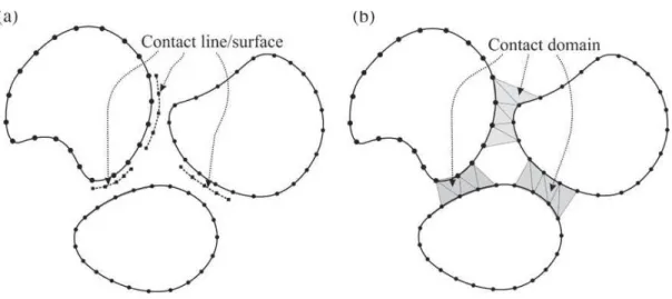
So, the difference between this method and the node-to-node or segment-to-segment strategy lays on the interpretation of the contact domain. In the classical methods, the contact conditions are formulated due to a projection of the contact surface or point (slave contact surface) onto the other contact surface (master contact surface), as shown in Fig. 3.3 (a). Considering that, the contact problem is a subdomain, with lower dimension. On the other hand, the contact mesh establishespatches, connecting the potential contact surfaces, in other words, an intermediate domain with the same dimension as the bodies in contact, Fig. 3.3 (b). (OLIVER et al., 2009, HARTMANN et al.,2009, HARTMANN et al., 2010, WEYLER et al., 2012)

In order to connect the potential contact surfaces, the patches created must not overlap, it must be a unique layer and it converge to the contact domain as the number of vertices increases. As shown on Fig. 3.4, the contact patches can be designed in multiples ways. In our study, we will use only tetrahedrical linear-linear shaped patches due to the best results in the contact formulation, according to Oliver et al. (2009).

element types are considered: Type A patches, with 3 vertex nodes placed on one contact boundary and one on the other and Type B, with 2 vertex nodes placed on each contact body. Type B elements are used to ensure that in 3D models all the contact domain is meshed. The 3D contact mesh, with both types of elements is shown in Fig. 3.5.

Figure 3.3. Imposition of contact constraints in: (a) Classical Methods; (b) Contact Domain Method. (Adapted from Oliver et al., 2009)

Fig 3.5. 3D Contact Domain approximated with Tetrahedral Elements. (Adapted from Hartmann et al., 2010)

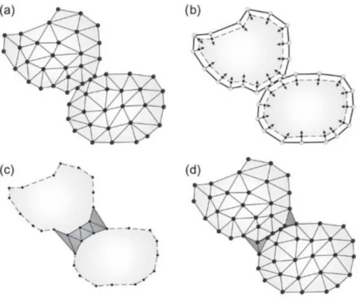
It is important to note that the creation of a contact mesh is independent of the master/slave relation, it means that it doesn’t matter which body will be considered as master or slave in the contact pair. The determination of the contact mesh, i.e., which points of each contact pair will be connected and when the mesh will be created is defined by an active strategy. So the creation process of the contact mesh follows 4 steps: i. the process starts with a FEM meshed pair of bodies, where the element chosen doesn’t affect the contact approach (Fig. 3.6 (a)); ii. the interior nodes are removed and the boundaries are shrunk (Fig. 3.6 (b)); iii. the contact mesh is created, linking both bodies in the probable contact areas (Fig. 3.6 (c)); iv. The original boundary and mesh are retrieved (Fig. 3.6 (d)). (HARTMANN et.al.,2010)

CHAPTER IV

CONSTITUTIVE MODEL FORMULATION

A microindentation experiment can be simulated as if the plastic deformations are greater when compared to elastic ones, enough to neglect the elastic part of the total deformations in the material formulation. Considering that, the formulation respected the big plastic deformation continuum mechanics theory, in whichthe process were considered purely mechanic, because in a quasistatic process, velocities are sufficiently low to neglect any heat or heat transfer.

4.1. Kinematic analysis

‰uv H ¡ ¢ . The process, microindentation or micro-scratch test, occurs in a

time interval£I ¤¥$œ$G_•, where _¤ is the final time of the process. (WEYLER, 2000) The deformation can be defined as _{$¦ §$<Y$A$£I ¤¥$€ G}ˆ•žŸ _{, so any}

particle of the body _{¨$ ©$<Y} in a given time _{‚$ © £I ¤¥} is ruled by the equation of motion (4.1), leading to a deformed body configuration given by the set of points _{<‘ H $¦ <Y ‚} , in time _‚. The equation (4.2) defines the displacement field (_.) from the equation of motion and equation (4.3) the deformation gradient tensor ( ) (WEYLER, 2000).

A H $6 ¨ ‚

. ¨ ‚ H 6 ¨ ‚ E ¨

¨ ‚ H

H & b

Where ª. « ‘

ª«

H ¬G-®$. ¨ ‚

To work with plastic deformation in elastoplastic materials, it must be considered that it goes through an elastic deformation stage before the permanent deformationstarts. This leads to the problem of coupling those two different deformation mechanisms of the material.

$¯ ¨ ‚ H ¯

_{¨ ‚ ± ¯}

_{¨ ‚}

An important consideration to be made is that the elastic part of the deformation is so small compared to the plastic part and it is possible to assume

¯ ² ¯°_{and ¯}• _{² ³. This leads to the assumption that the effects of rotation in the}

rigid body movement are not great enough to cause major errors. In the reference configuration _´Y , the Cauchy Green tensor is given by the equation (4.5) and then the Green Lagrange deformation in shown in the equation (4.6).

H

H

E &

In the deformed configuration _´‘, the Finger deformation tensor _µ D is given by the equation (4.7) and its elastic part _¶µ•†S_· is given by the equation (4.8), where _¬¸ is the metric tensor related to the intermediate configuration and

¬ is the metric tensor related to the material configuration.

µ

_{A ‚ H}

_¦

_{A ‚ ‚ ± ±}

_¦

_{A ‚ ‚}

µ

_{¨ ‚ H}

_¦

_{A ‚ ‚ ± ±}

_¦

_{A ‚ ‚}

» A ‚ H

¶º E µ

_{A ‚ · H »}

_{A ‚ b »}

_{A ‚}

»

_{A ‚ H}

F

Kº E µ

†S

A ‚ R

»

_{A ‚ H}

Kµ

†S

A ‚ E µ

_{A ‚ R}

4.2. Incremental Formulation

The incremental formulation aims to determine the internal and dependent variables from the free and boundary variables (Total deformation, Plastic deformation and internal variables). For that, the time is subdivided in incremental steps £I ¤¥ H ¼ £‚ˆ½_{ˆ¾Y ‚ˆ•D¥}. Also for all the particles belonging to the domain

¨$ © ´Y , it is known the displacement field 3¿ˆ•DÀ ´Y € GˆrÁ in the time

increment _{£‚ˆ ‚ˆ•D¥} and the variables _{æˆ `ˆ}° _?ˆÄ at _‚ˆ, where _?ˆis the stress field in the initial configuration. The Integration will consist in determine the variables

戕D `ˆ•D° ?ˆ•DÄ$at ‚ˆ•D. Once these variables were determined, all the other

ones are automatically determined aswell. (WEYLER, 2000)

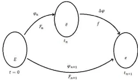
Figure 4.1 represent the incremental formulation design, where is the deformationin the initial configuration of the body, _$is thedeformation in the final configuration and is the deformation in an intermediate stage defined by _‚ˆ.

To relate material tensors with spatial tensor it is used the transfer operators _{XÅÆƵ’ÇÈ$É} and _{$XÅÊË@ÌÍm’Í•$É} , which can use the transformation

final configuration _@ and from the final configuration to the last converged one

@ D _.

Figure 4.1. Representative design of the incremental formulation.

H

ªÎ

H $ b

ª6

H

H $ E

The Finger tensor, in the intermediate configuration, is now in the form of the equation (4.14), its elastic part the equation (4.15) and the additional split of the Almansi tensor, also in the intermediate configuration and isolated for the elastic part, is shown by the equation (4.16).

H E ¡

H E ¡

4.2.1 Predictor-corrector algorithm

The time integration uses a predictor-corrector algorithm, and for that the integration is composed by two stages. In the first stage, is calculated an elastic prediction, as known as trial, in which the irreversible variables are frozen, such as the internal variables. The second stage works as a plastic correction, where the solution of the first stage is corrected back to the yield surface if it's out, in other words, until the Kuhn-Tucker conditions are satisfied. (WEYLER, 2000)

The process starts with the calculation of the Almansi tensor in the intermediate stage at _‚ˆ•D, equation (4.17), by applying a pullback(transforming to the equation material form) in_{$ •} and then in equation (4.18), calculate the trial of elastic part of the Almansi tensor at _‚ˆ•D, applying a pullback at _• . The equation (4.19) shows the trial of the elastic part in the deformation tensor. With the equations (4.17), (4.18) and the additional split, shown at equation (4.16), it is possible to calculate the plastic part of the Almansi tensor in the intermediate stage, equation (4.20). From the equation (4.20) it is possible to notice that the plastic part of the Almansi tensor at the initial configuration (which is an input data) stays the same for the other two configurations and also for the trial at _‚ˆ•D.

•

H É

H

± E

•

H É K

R H

± E

Where

•

H

$±

E

With the result from the equation (4.20), the stress tensor, the internal variables and the yield surface is possible to calculate a function _ÐÑP _X , that determines if the current equivalent stress is still inside the yield surface _ÐÑP _‡

I , which means that the trial responses are the actual values for the time step

‚ˆ•D. In the case that the current equivalent stress is outside the yield surface ÐÑP_{Ò I , there must be calculated the return of this point to the yield surface}

border, and then use the values obtained. In both cases, to obtain the values of the Almansi tensor and the plastic part of the Almansi tensor, the push-forward

operator must be applied, as presented by the equations (4.21) and (4.22).

•

H Ó Ô

H Ö

± Ô

± Ö

•

H Ó ¶Ô

· H Ö

± Ô

± Ö

CHAPTER V

YIELD SURFACE AND HARDENING LAW

Yield surface is defined as a map in stress space, in which is drawn a boundary that separate non-yielded regions from the ones that already undergo flowing due to the problem conditions.(COURTNEY, 2005)

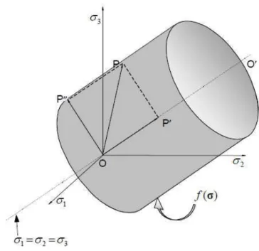
The yield will be the criteria to define a material plasticity, according to the equation (5.1), in which the first term represents a function of stress tensor and hardening variables. Considering an isotropic material, the yield depends only on the principal stresses, so the Ffunction becomes dependent only on the scalar hardening _{Ø ™}. (NATAL JORGE, 2004)

¯ ™ H @

E ?

™ H I

Figure 5.1- Westergaard space (JORGE NATAL, 2005)

The increment of the point _Ú is represented by the vector _CÚÛÛÛÛ, which can be decomposed and its components coincide with the hydrostatic stress(axis where the three principal stresses has the same value) and the deviatoric stress , where _CÚÜÛÛÛÛÛ is normal to _CCÝ. So the yield will depend only on the vector _CÚÜÛÛÛÛÛ (shape changing stresses or deviatoric stresses). This is only true if the hydrostatic pressure (volume changing stresses) does not affect the material yield, which can be demonstrated by experimental tests. Given that, the yield will depend only on the second and the third invariants of the deviatoric stresses (Sij),

shown in the equations (5.2) and (5.3).(JORGE NATAL, 2005, KACHANOV, 1974)

ÞF

H

‚Í ß

_H

F

àvwà

ÞV

H

‚Í ß

_H

V

àvwà

á H

Ê»‰

_âE

Fã_NST

ä$y $$á$ © åE

$ b

]

O

æ

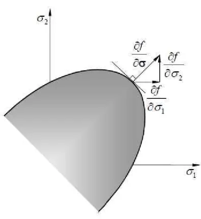
Considering a deformable material, if_{$@ ç ?Ù ™} , the analysed point is showing elastic behaviour. On the other hand, if _{@ H ?Ù ™} , the material behaviour is considered plastic. The material behaviour after that point will depend on the _@ variation due to , as shown by the equation (5.5), which is a vector normal to the yield surface called associated plastic flow, Fig. 5.2.

•@ H K

R

• b x

In summary,

• If •@ ç I, the material shows elastic behaviour and the incremental stress

is located inside the yield surface.

• If •@ H I, the material shows perfectly plastic behaviour, constant ™, and

the stresses are located on the yield surface boundaries.

• If •@ Ò I, the material is undergoing hardening, which means that the yield

Figure 5.2 – Orthogonally Condition in _{?DE ?F} space (JORGE NATAL, 2005)

5.1. Von Mises Yield Surface

According to Von Mises (1913), the yield occurs when the second invariant of the deviatoric stresses _ÞF reaches a critical value, depending on the hardening

™ . This hypothesis considers the distortion energy density and should be true for an uniaxial stress state aswell, where _{Ó è H š}F_V?Ù and the effective stress is given by the equation (5.6).

?Û H é¢Þ

H š

ßÀ ß H š

à

à

$$€$$?Û E ?

™ H I

According to Hill (1950), the deformation energy in terms of the second deviatoric and the volumetric expansion (equation (5.7)) will only ensure incompressibility if the Poisson Ratio _c is iqual to 0.5 and therefore the second part of the equation (5.7) will became null, resulting in the equation (5.8).

¿

H

Þ

b

?

¯ ™ H

Þ

E

?

™ H I

The equation (5.6) and (5.8) can be combined, resulting in the effective stress in terms of the second deviatoric stress _ÞF (equation (5.9)), which shows that Von Mises yield surface is applicable to materials with no volumetric deformation.

5.2. Ludwik Nadai hardening law

After the analysis of the deformation being inside or outside the yield surface, it becomes necessary to understand and prescribe the hardening experienced by the material when it goes under plastic deformation. Many are the mathematical models with the purpose of describe the behaviour of the hardening curve and for this work were used the Ludwik-Nadai hardening law. (MELCONIAN, 2014)

This law is exponential and considers the variation of the plastic deformation, as it can be seen on equation (5.10).

?

H 馓

E ì

·

Where,

• ?_Ù is the yield stress

• È is the hardening modulus

• ì_°íY is a initial equivalent plastic strain that defines the initial yield stress • ì°íis the current equivalent plastic strain.

• ‰is the hardening exponent.

The current stress value is equal to the yield stress when the current plastic deformation is equal to zero, as given by the equations (5.11) and (5.12)

ì

H K

R

S

• _(5.11)

? H È ïK

ƒ

R

S •

_{E ì}

°í

ð

H È ïK

ƒ

R

S

•

_{E Ið}

_{H ?}

CHAPTER VI

INSTRUMENTED MICROINDENTATION

According to Jost (1966), Tribology is the science field which studies contacting surfaces, in relative motion, and related subjects. This concept unifies the friction, lubrication and wear subjects in only one field of study. This is important, considering that the wear phenomenon is a complex interfacial process, which is irreversible, progressive and with difficult theoretical characterization. (NOGUEIRA, 1988, MARTINS, DA SILVA, 2008)

Aiming to comprehend and predict the wear, more specifically the abrasive wear phenomenon, experimental simulations are often used. These simulations are divided in two groups:

i- Global Approach, which tries to represent the abrasive wear in an area, using abrasometric techniques. (Costa et al., 2001, FRANCO et al.,

1989);

6.1. Microindentation Test

The microindentation test consists in an experimental method in which the specimen is pressed by a known shaped indenter, with controlled load and displacement. Analysing the load, displacement and also the indentation mark, it is possible to calculate the bulk or multi-layered materials properties. It is also possible tocharacterize the multi-layered material adhesion between layers and analyse other phenomena, such as the pile-up and sink-in. (GU et al., 2003, FELICE NETO, 2012, RUTHERFORD,1997, CHEN, 2007, HOLMBERG, 2009)

The microindentation test schematic diagram is represented inFig. 6.1.

The microindentation experiments carried by Da Silva (2008) gave as results for microindentation depth vs. Applied Force, for 5N and 10N Brinell indenter experiment, the Fig. 6.2 and 6.3 respectively. For the Brinell indenter, the standard used was ASTM E10-15a.

It is important to note that the curve separates from zero in the X axis only with 8 µm depth, which means the indenter approximation, i.e., the indenter does not start touching the specimen and the total depth actually is the subtraction between the greatest value for depth and the value where the force became different from zero, approximately 7 and 15µm, for 5N and 10N experiment respectively.

Fig.6.2. 5N Brinell Microindentation Force vs. Depth curve (DA SILVA, 2009)

Fig. 6.3. 10N Brinell Microindentation Force vs. Depth curve (DA SILVA, 2009)

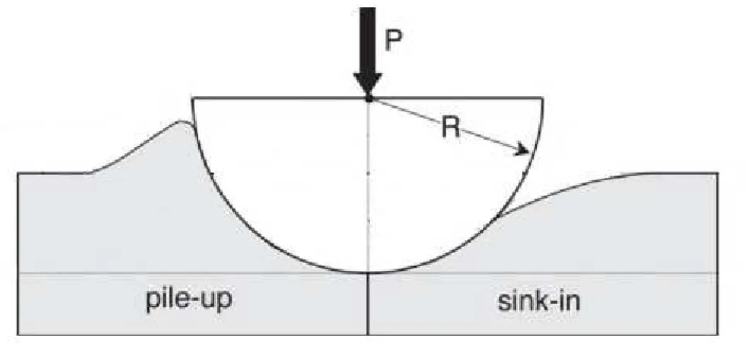
6.2. Pile up and Sink in

Fig. 6.4. Pile up and sink in phenomena. (Adapted from TALJAT & PHARR, 2004)

6.3. Laser Interferometry

The laser interferometry is a measurement method which uses wave interference to measure distances. A laser beam is divided in two and each beam goes through a different path. The first beam goes to a reference mirror and the second to the specimen surface and then both lasers are reflected together to a detector. The difference in the wave pattern is calibrated to indicate distances and, therefore, the specimen surface roughness. (BUSHAN, 2001)

Fig. 6.5. Schematic Design of the Laser Interferometry operation mechanism (UBM, 1999)

There were also scanned with Laser Interferometry a Copper Specimen with 10N load and the same 2.5 mm indenter diameter. Figures 6.8 and 6.9 show the Copper specimen topography and roughness profile for this experiment. (DA SILVA, 2008)

Fig. 6.6. Laser Interferometry of the 5N Brinell microindentation (DA SILVA, 2009)

Fig. 6.8. Laser Interferometry of the 10N Brinell microindentation (DA SILVA, 2009)

CHAPTER VII

METHODOLOGY

In the previous chapters were discussed the contact problem, theoretically and numerically. After that, were discussed material plastic properties and a formulation (material and contact) to simulate severe contact conditions, such as the microindentation test, reviewed in Chapter 6. This Chapter aims to stablish a methodology to create a contact domain approach in Explicit FEM, inside an existing program, create a Small Elastic and Large Plastic Deformations formulation, validate the method using experimental tensile strength test and simulate a microindentation test.

7.1. Implementing the Constitutive Model in COMFORM

constitution, making possible to introduce new modules that works with the already existent programming.

The COMFOM software, before this work, was capable of simulating axisymmetric, 2D and 3D problems, with triangular or quadrilateral mesh, all with implicit time integration. The code can be used to simulate general mechanical process, such as stamping, bending, contact and also sintering. To do so, the software uses elastic, plastic, granular and powder material formulations.

Considering the microindentation problem, where the deformation is really punctual (micrometres), the elastic part of the total deformation is small enough to be neglected, and then all the deformation is considered to be plastic. Thus, a Small Elastic Large Plastic (SELP) constitutive law was implemented in the COMFORM software. This material behaviour works now in all implemented modulus.

The second stage was to implement the explicit time integration inside COMFORM, using the methodology from Chapter III. The Explicit Method were also implemented to work with all modulus of COMFORM (2D/3D, material formulations, mesh criteria).

Then, convergence tests were made, just to be sure that the entire system works. After the convergence tests, a validation test were made for a tensile strength experiment.

7.2. Validation of the Implemented Model

The software COMFORM is a calculus module only, i.e., it doesn’t have an interface to create geometry, mesh, boundary conditions and read the post-process data. For that, were used the GiD platform, which provides several tools to build the pre-process and post-process data, including a problem type feature, that enables the user to create a standard data export, making easy to create COMFORM structure data file.

Using the GiD software, were designed two models, with square shaped cross-section area and same length as the experimental test (_ŠII$ññF and

òI$ññ respectively). The square shaped cross-section area is different from the experimental specimen cross-section, which is circular, but if the cross-section area is the same, the Stress vs. Strain and Force vs. Displacement curves won’t differ. The difference between the models is the element mesh, the first model used tetrahedral and the second hexahedral elements, as shown in Fig. 7.1

Fig. 7.1 Tensile Strength FEM models with Tetrahedral and Hexahedral Elements.

Fig. 7.2. Distribution of nodes in the top surface of the tensile strength experiment test model.

experimental tensile strength test was 7000 [N], the Equation 7.1 shows the distribution of the force through the elements on the surface.

Šó± Š±ô_¯ÌÍÇ»ô _{b Šó± I ò±}ô_¯ÌÍÇ»ô _{b õ± I ¡ò±}ô_¯ÌÍÇ»ô _{H öIII$£÷¥ (7.1)}

So, the curve that represents the Force (F = 280 N) vs. Time that were imposed in the surface elements is shown by Fig.7.3.

Fig. 7.3. Time vs. Force curve applied to the tensile strength test top nodes. For the Tetrahedral mesh model, were used a similar approach to distribute the Load trough the top surface elements, considering that the tetrahedral mesh has more elements even with the same number of division in each axis. That can be seen on Fig. 7.1.

7.3. Material properties from tensile strength test curve

The tensile strength test provides some material properties directly from the experiment and other properties are given by the bulk material manufacturer, those properties are listed in Table 7.1.

Table 7.1 Copper specimen properties.

Property Value Unity

Young Modulus (E) 117 GPa

Yielding Stress ( ₀) _110.83 MPa

Poisson’s ratio (_; 0.3 -

Density (>) 8960.0 Kg/m³

Those properties doesn’t concern to the plastic deformation hardening and for this phenomenon must be used a hardening model. For this work were used a Ludwik-Nadai model, an exponential hardening law, which performs a good hardening representation of several materials, including Copper. The Ludwik-Nadai hardening law is presented by the equation (5.11).

The plastic part of the deformation can be calculated for the tensile strength test using the initial specimen length _ÆY and the displacement trough the experiment. In this case, the Plastic part of the deformation starts in zero and increases during the experiment, in the form of the equation (7.3). The differential plastic part of the deformation is in the form of the equation (7.4).

ì

H ì

b 3ì

¶3ì°·

H Š±ò± ì

E ì

b ¡± ì

E ì

S N

Where

ì

H I±ò± ïŠ E Z

_

ð

ì

H I±ò± ïŠ E Z

_ð

And _Æ{ is the final length of the specimen.

Using those equations and the experimental curve Force vs. Displacement, it is possible to create a MatLab® minimization function, in which a seed of k (hardening modulus) and n (hardening exponent) is chosen by the user and the function minimize the error (difference between the calculated and experimental stress) in order to approximate the two curves. It considers a number of evaluations and an error tolerance. The initial seed were chosen considering a common Copper material found in the literature and the evaluations started in 100 (default) until the response value of k and n does not change anymore (400 evaluations). The algorithm returns the values of k and n for the minimum calculated error and the complete implemented MatLab® algorithm is presented in the APPENDIX A.

7.4. Simulation of a Micro-indentation test

To decrease the simulation time, the microindentation model created is a quarter of the whole model, i.e., symmetry in the XZ and YZ plans. The indenter is sphere shaped with 2.5 [mm] diameter and has only the tip of the indenter designed, considering that the indenter won’t undergo plastic or large elastic deformations because it is constituted by a hard material (tool steel), when compared to the copper specimen (designed with _{I±ö$A$I±ö$A$Š±õ$ññ}). Figure 7.4 shows the simulation model created for the microindentation test and Tab. 7.2 shows the indenter elastic properties.

Fig. 7.4. Representation of the microindentation test. Table 7.2. Microindentation Simulation Indenter properties.

Property Value Unity

Young Modulus (E) 210 GPa

Poisson’s ratio (_; 0.3 -