A method for sea ice thickness and concentration analysis based on SAR data and a thermodynamic model

www.the-cryosphere.net/6/1507/2012/ doi:10.5194/tc-6-1507-2012

© Author(s) 2012. CC Attribution 3.0 License.

The Cryosphere

A method for sea ice thickness and concentration analysis based on

SAR data and a thermodynamic model

J. Karvonen1, B. Cheng1, T. Vihma1, M. Arkett2, and T. Carrieres2 1_{Finnish Meteorological Institute (FMI), Helsinki, PB 503, 00101, Finland} 2_{Canadian Ice Service, 373 Sussex drive, Ottawa, Ontario K1A 0H3, Canada} Correspondence to:J. Karvonen (juha.karvonen@fmi.fi)

Received: 2 April 2012 – Published in The Cryosphere Discuss.: 31 May 2012

Revised: 9 November 2012 – Accepted: 20 November 2012 – Published: 14 December 2012

Abstract.An analysis of ice thickness distribution is a chal-lenge, particularly in a seasonal sea ice zone with a strongly dynamic ice motion field, such as the Gulf of St. Lawrence off Canada. We present a novel automated method for ice concentration and thickness analysis combining modeling of sea ice thermodynamics and detection of ice motion on the basis of space-borne Synthetic Aperture Radar (SAR) data. Thermodynamic evolution of sea ice thickness in the Gulf of St. Lawrence was simulated for two winters, 2002–2003 and 2008–2009. The basin-scale ice thickness was controlled by atmospheric forcing, but the spatial distribution of ice thick-ness and concentration could not be explained by thermody-namics only. SAR data were applied to detect ice motion and ice surface structure during these two winters. The SAR anal-ysis is based on estimation of ice motion between SAR image pairs and analysis of the local SAR texture statistics. Includ-ing SAR data analysis brought a significant added value to the results based on thermodynamics only. Our novel method combining the thermodynamic modeling and SAR yielded results that well match with the distribution of observations based on airborne Electromagnetic Induction (EM) method. Compared to the present operational method of producing ice charts for the Gulf of St. Lawrence, which is based on visual interpretation of SAR data, the new method reveals much more detailed and physically based information on spa-tial distribution of ice thickness. The algorithms can be run automatically, and the final products can then be used by ice analysts for operational ice service. The method is globally applicable to all seas where SAR data are available.

1 Introduction

the Finnish ice charts show the ice concentration, the mean, maximum and minimum ice thickness, as well as the spa-tial distribution of different ice types. In addition, the level of ridging is characterized by a number from 1 to 5. In the Cana-dian Ice Service, the ice chart is in the form of the WMO egg code (Sandven and Johannesen, 2006) presenting the con-centration, stage of development, and predominant forms of up to 3–5 ice types for each selected geographical area. The Chinese ice charts for the Bohai Sea illustrate the isolines of ice thickness and ice edge as well as the ice drift velocity field (Luo et al., 2004).

In large sea areas with little navigation, remote sensing is the most powerful tool to collect information needed for an ice analysis, but challenges still remain. These depend on the type of remote sensing data available. In the case of passive microwave data, the detection of ice concentration is a challenge when it exceeds approximately 85 % (Ander-sen et al., 2007). Retrieval of high ice concentrations by mi-crowave radiometers is degraded by surface effects, sensor smearing and sensor noise. The development of Synthetic Aperture Radar (SAR) methods have yielded a lot of ad-vance, but problems still exist, among others, in the detection of ridges and measurement of ice thickness and above all in the discrimination between thin and thick ice when both are deformed (M¨akynen and Hallikainen, 2004; Shokr, 2009). Also, discrimination of sea ice from open water based on SAR signature is complicated by the ambiguities in the SAR signature of sea ice in comparison to the SAR signature of open water. The SAR signature of open water is a function of the size of the openings and the prevailing wind conditions. However, methods utilizing texture features have yielded bet-ter results in SAR-based open wabet-ter detection, these methods have been described, for example, in Karvonen et al. (2005, 2010).

The challenges in ice analysis also depend on the local conditions. The analysis is more difficult if the ice thick-ness and concentration are strongly affected by both ther-modynamics and dynamics. In seasonally ice-covered seas, the production of ice (basin-scale temporal evolution of ice thickness) is typically dominated by thermodynamic pro-cesses; the air–ice–ocean thermal interaction is crucial to determine the columnar and granular ice growth (Bitz et al., 2001) (columnar growth is due to freezing of sea wa-ter, whereas granular growth is due to refreezing of melted snow). The spatial distributions of ice thickness and con-centration are, however, often dominated by ice dynamics (Fichefet and Maqueda, 1997). A preliminary investigation of ice thickness analysis based on SAR data and a thermo-dynamic ice model has been made for the Baltic Sea (Kar-vonen et al., 2007, 2008). Also, the RADARSAT geophysi-cal processor system (RGPS) (Kwok, 1998) has utilized the thermal growth to estimate the ice thickness distributions of Lagrangian cell ice age classes. The RGPS ice age classes are computed based on the ice drift between to adjacent SAR images over the same area. The method used in RGPS

re-quires reliable tracking of each Lagrangian cell from image to image in time. In practice, this kind of tracking using avail-able SAR data, e.g. for Gulf of St. Lawrence, is not possible because of too sparse temporal coverage. In addition, the lo-cal SAR backscattering dynamics is attenuated by occasional above-zero temperatures, and for this reason the SAR images typically contain less textured areas for which meaningful correlations between pairs of SAR images can be obtained and reliable ice drift estimates be given. Due to these restric-tions, our approach for ice parameter estimations is different from the RGPS.

In this study, a new method is presented for sea ice thick-ness and concentration analysis based on SAR data and a thermodynamic model. Here, we address the seasonal sea ice cover in the Gulf of St. Lawrence (GSL) off Canada, but the methodology is applicable for all ice-covered seas with weather forcing and SAR data available. In the GSL the ice cover is more dynamic than in the Baltic Sea. Hence, the SAR-based method for the Baltic Sea (Karvonen et al., 2007, 2008) cannot be directly applied for the GSL, be-cause ice motion detection from SAR data is also needed. First we present a new method to derive sea ice concentra-tion and drift vectors on the basis of SAR data. In locaconcentra-tions where the SAR data indicate presence of sea ice, a thermo-dynamic sea ice and snow model HIGHTSI is used to calcu-late the ice growth, forced by operational model products of the European Centre for Medium-Range Weather Forecasts (ECMWF). The thermodynamically based ice thickness is used as background information for the remote sensing al-gorithm. For the first time, we combine the SAR-based in-formation and thermodynamic modeling of sea ice and its snow cover. The resulting sea ice thickness and concentra-tion analyses are finally compared against airborne Electro-magnetic Induction (EM) measurements and the present op-erational products of the Canadian Ice Service (CIS).

2 Study area, ice seasons, and data

The GSL is a seasonally ice-covered gulf at latitudes as low as 45.6–52.0◦N (Fig. 1). Winter navigation in the GSL is active, as it is the pathway to St. Lawrence River provid-ing access to Quebec City, Montreal, and the North Amer-ican Great Lakes. Due to the high economic importance of navigation, there is a strong need to provide accurate sea ice analysis for the GSL. The dynamic sea ice cover in the GSL represents a challenging environment for ice analysis.

Fig. 1.The Gulf of St. Lawrence and surroundings plotted in Lam-bert Conformal Conic (LCC) projection. The ice analysis domain is the red-dotted sea area; each dot corresponds to one grid cell of the ice model. The original model domain is computed in latitude– longitude and then converted to LCC. The corner latitudes and lon-gitudes of the original grid are shown. The ice model simulations are made at each grid cell for the two winter seasons.

11 May 2009. We had comprehensive data sets and sup-porting material covering both ice seasons from freeze-up to melt: SAR data, CIS ice charts, ice thickness measure-ments based on the EM device (Prinsenberg et al., 2002), and numerical weather prediction (NWP) products from the ECMWF. The SAR data consisted of 149 RADARSAT-1 im-ages from 2002–2003 and 250 RADARSAT-2 imim-ages from 2008–2009. The RADARSAT data were georeferenced level 1b SAR data. RADARSAT-1 data were in CEOS format, and RADARSAT-2 in GeoTIFF format with supplementary XML files. The data were received from CIS for this par-ticular experiment. Both RADARSAT-1 and RADARSAT-2 operate at C-band (wavelength 38–75 mm); the wavelengths are 56 mm for RADARSAT-1 and 55 mm for RADARSAT-2 (slightly modified from that of RADARSAT-1 due to inter-ference of RADARSAT-1 frequency with WLAN frequen-cies). The SAR images were ScanSAR images, which are made about 500 kilometres wide by combining several SAR beams. Because of the wide spatial coverage, these images are most suitable for operational sea ice monitoring. The tem-poral coverage, i.e. the time difference between updating of SAR data at a given location within the study area, was about 1–3 days for the season 2008–2009 and 1–4 days for 2002– 2003.

The CIS ice charts were in a gridded format. The ice charts are primarily based on visual interpretation of satellite

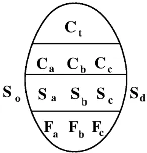
im-Fig. 2.The WMO egg code given for each polygon (area).Ctis the total concentration;Ca,Cb, andCcare the fractional concentra-tions;Sa,Sb, andScare the fractional stages of development cor-responding to the fractional concentrations; andFa,Fb, andFcare the fractional predominant forms of ice.SoandSdare the stages of development of the possible remaining ice types within the the area. All three fractional values are not necessarily assigned for each polygon if there are less ice types present according to the ice ana-lyst interpretation.

agery and ice reconnaissance flights. The ice conditions are qualitatively illustrated by the standard WMO egg code over polygons defined by the CIS ice analysts in various parts of the GSL. A diagram of the WMO egg code is given in Fig. 2. The CIS ice charts are drawn daily and they rely on EO data and ship and aircraft observations. RADARSAT SAR data with a wide coverage are their major data source. For making ice charts the SAR data is first analyzed and then a forecast (nowcast), based on other sources of information (including other EO data, ice reports from ships), is made. The CIS ice charts have not been systematically verified objectively, but they represent the best and most accurate ice information available in GSL. The daily CIS ice charts are issued at 18:00 UTC. They at least give a qualitative description of the pre-vailing ice conditions. Additionally, we have also tried to use the ice charts for quantitative evaluation by using the total ice concentration and the ice thickness ranges given by the stage of development for each CIS ice chart segment (defined by the bounding polygons drawn by the ice analysts).

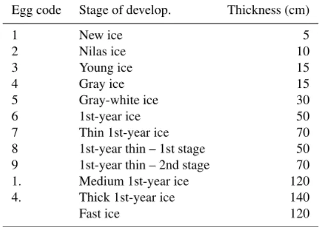
Table 1.Conversion from the egg-code stage of development into ice thickness used here. The multi-year ice types have been ex-cluded.

Egg code Stage of develop. Thickness (cm)

1 New ice 5

2 Nilas ice 10

3 Young ice 15

4 Gray ice 15

5 Gray-white ice 30

6 1st-year ice 50

7 Thin 1st-year ice 70

8 1st-year thin – 1st stage 50

9 1st-year thin – 2nd stage 70

1. Medium 1st-year ice 120

4. Thick 1st-year ice 140

Fast ice 120

ice. The segment total concentration valueCt was used as the concentration value in the comparisons. The ice thickness was derived from the stage of development, and we have here used the lower boundary of the ice thickness ranges given by the stage of development. For each ice chart segment, the stage of development corresponding to the most frequent fractional concentration is used in the mapping of ice ness. In the case of multiple ice types with different ice thick-ness ranges present within one ice chart segment, the used ice thickness mapping may to some extent deviate from the mean of the ice thickness lower boundaries computed based on the ice chart fractions of the different ice types.

The quantified daily ice charts were interpolated to the HIGHTSI model domain (3111 grid cells, Fig. 1) and the ice thickness and concentration from each grid cell were ex-tracted on each day. Due to the dynamic sea ice cover in the GSL, the spatial distribution of ice thickness at a given time step is very complex and difficult to assess. The seasonal ice evolution, however, can be illustrated by the integrated basin-scale mean daily ice thicknessHa and daily total ice cover areaHA:

Ha(t )= 1

N N X

i=1

Hi(t ) and (1a)

HA(t )= 1

N N X

i=1

(GiCi(t )), (1b)

where Hi is the ice thickness in the grid cell i, N is the total number of grid points in the model domain,t is the time (day),Ci is the ice concentration, and Gi is the grid celli area. Figure 3 shows the quantified CIS-based daily time series of ice area as well as maximum and minimum basin-scale ice thicknesses for winter seasons 2002–2003 and 2008–2009.

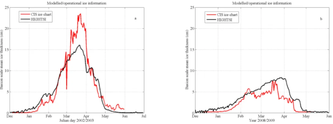
Ice winter 2002–2003 was severe. The maximum values of ice area and mean basin-scale ice thickness occurred in late March. In the early freezing season, the ice cover developed faster with respect to area than thickness; from 1 January to 1 February, the ice area increased by 11 times whereas the ice thickness only increased by 5 times. During the melting sea-son, however, ice thickness and area decayed with the same rate. Ice winter 2008–2009 was milder; in early winter the ice area increased faster than ice thickness. After the maximum ice cover was reached, the ice area and thickness varied with the same rate until the final ice melt. Compared with winter 2008–2009, the maximum ice area in winter 2002–2003 was almost 3.5 times as large and the basin-scale sea ice mean thickness was 3.1 times as thick. The maximum ice area and mean ice thickness appeared in mid-March to be in line with the ice climatology in the GSL.

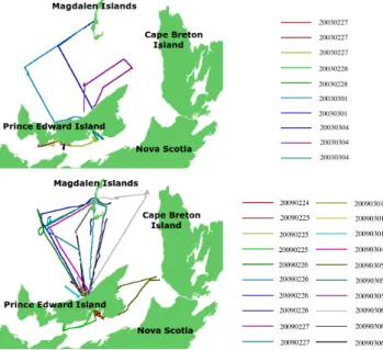
The electromagnetic induction (EM) (Prinsenberg et al., 2002) ice thickness measurements have been carried out over the GSL during several seasons. The measurements for the two particular seasons studied in this experiment were used as a reference ice thickness data set. EM measurements are considered as one of the most accurate methods to measure sea ice thickness over a large area that cannot be covered by drilling (Pfaffling et al., 2006; Haas et al., 2006). In both the winters 2002–2003 and 2008–2009, the EM measurements were made within a relatively short period of 1–2 weeks from late February to early March. The measurements were made close to the Prince Edward Island, and were mainly headed to the north of the island (Fig. 4). The sampling rate of the EM measurements was 3–4 m and the resolution (footprint) was around 20–30 m. The EM flight lines used in this study with their acquisition dates shown by color codes are shown in Fig. 4.

3 Thermodynamic modeling

3.1 HIGHTSI model

A high-resolution thermodynamic snow and ice model (HIGHTSI) is used in this study to simulate thermody-namic ice growth and melt. HIGHTSI was initially devel-oped to study snow and ice thermodynamics in seasonally ice-covered seas (Launiainen and Cheng, 1998; Vihma et al., 2002; Cheng et al., 2003, 2006). The model has been further developed to investigate snow and sea ice thermodynamics in the Arctic (Cheng et al., 2008a,b) and also lake ice (Yang et al., 2012; Semmler et al., 2012).

Table 2.Conversion from the CIS egg-code total concentration (Ct, given in tenths) into ice concentration shown in this paper. The egg-code labels OW (open water) and IF (ice-free) are converted to 0 % and FAST (fast ice) to 100 %.

Egg code 1 1+ 2 2+ 3 3+ 4 4+ 5 5+ 6 6+ 7 7+ 8 8+ 9 9+ 10

Concentr. (%) 10 15 20 25 30 35 40 45 50 55 60 65 70 75 80 85 90 95 100

Fig. 3.Time series of daily basin-scale minimum and maximum ice thickness and ice area retrieved from operational CIS ice charts for winters(a)2002–2003 and(b)2008–2009. The CIS ice chart gives a range for the daily minimum ice thickness in the domain (see Fig. 1) and another range for the maximum. The minimum and maximum thicknesses are the means of these ranges. The ice area is the total ice-covered area in the domain.

Fig. 4. The EM flights in 2003 (upper panel) and 2009 (lower panel). The flight dates are shown by the colors.

the snow and ice depends on the cloud cover, albedo, color of ice (blue or white), and optical properties of snow and ice. The shortwave radiation penetrating through the surface layer is parametrized, making the model capable of quantita-tively calculating sub-surface melting. Short- and long-wave radiative fluxes can either be parametrized or prescribed

based on results of numerical weather prediction (NWP) models. The surface temperature is then solved from a de-tailed surface heat/mass balance equation, which is defined as the upper boundary condition and also used to determine whether surface melting occurs. At the lower boundary, the ice growth/melt is calculated on the basis of the difference between the ice–water heat flux and the conductive heat flux in the ice. The ice–water heat flux (refers to oceanic heat flux in this study) is assumed as a constant.

Model experiments in the Arctic Ocean have suggested that albedo schemes with sufficient complexity can more re-alistically reproduce basin-scale ice distributions (Liu et al., 2007). We applied a sophisticated albedo parametrization ac-cording to temperature, snow and ice thickness, solar zenith angle and atmospheric properties (Briegleb et al., 2004). The thermal conductivity of sea ice is parametrized according to Pringle et al. (2007), and snow density and heat conductivity are calculated according to Semmler et al. (2012).

3.2 Forcing data and studied winter seasons

The atmospheric forcing for HIGHTSI was based on the op-erational analysis and short-term forecasts of the ECMWF. The reason for applying ECMWF products is their global availability. This is essential as we want to develop an ice analysis method applicable in all ice-covered seas. The anal-yses were available with 6-h intervals. The 2 m air tempera-ture and humidity as well as the 10 m wind speed were ap-plied to parametrize the turbulent fluxes of sensible and la-tent heat. The downward components of the solar shortwave and thermal long-wave radiation were based on 12-h opera-tional forecasts. To avoid spin-up problems in precipitation (Tiet¨av¨ainen and Vihma, 2008), snow fall was based on 24-h forecasts. We selected the ECMWF products as forcing for HIGHTSI because previous studies have demonstrated that the accuracy of ECMWF products is high compared with other re-analysis data, such as NCEP/NCAR, at high lati-tudes (Bromwich et al., 2009; Cheng et al., 2008a; Jakobson et al., 2012). To get an idea of the accuracy of the ECMWF products in the GSL, the wind speed (Va) and air temperature (Ta) at selected locations were compared with results of the Environment Canada regional operational forecast model (in 15 km resolution). The results of the ECMWF and Environ-ment Canada models agreed very well. The correlation coef-ficient between ECMWF and CIS modeled basin-scale wind speed and air temperature were 0.97 and 0.98, respectively, for both winter seasons. The temporal standard deviation of ECMWF and CIS wind speed was the same within 0.1 m s−1 both in winter 2002–2003 and 2008–2009. For temperature, the standard deviations were 5.0◦_{C (ECMWF) and 5.4}◦_C (CIS) in winter 2002–2003 and 4.8◦C (both ECMWF and CIS) in winter 2008–2009. The basin-scale ECMWF mean air temperature for the entire winter seasons of 2002–2003 and 2008–2009 were−2.1◦C and−0.8◦C, while the corre-sponding values from CIS regional model were−2.9◦C and −1.2◦C, respectively. The mean wind speed for the winter 2002–2003 from the ECMWF result was 8.4 m s−1 versus 8.0 m s−1 from the CIS regional model. For winter 2008– 2009 the corresponding values were 8.6 m s−1 (ECMWF) and 8.3 m s−1(CIS). The wind direction is not investigated as HIGHTSI does not include ice dynamics. As a summary, ei-ther of the atmospheric models could have been used to pro-vide forcing for HIGHTSI. We selected the ECMWF model because of our objective to develop a globally applicable method for sea ice analysis.

To carry out HIGHTSI simulations over the entire GSL, at-mospheric forcing is needed over a high-resolution grid. The ECMWF analysis and forecasts were available with a hori-zontal resolution of 0.358◦for winter 2002–2003 and 0.225◦ for winter 2008–2009, whereas HIGHTSI was applied in a resolution of 0.225◦ in longitude and 0.1125◦ in latitude. Hence, the ECMWF forcing fields were linearly interpolated to the HIGHTSI grid.

3.3 Model simulations

HIGHTSI simulations were carried out at each of the 3111 grid cells. Each model run starts 1 December and lasts until 31 May. The simulations are initialized with a thin ice layer (0.01 m) at each grid cell. The ice thickness is calculated as a mean over the ice-covered area in the grid cell. During the simulation, if the external weather data do not favor ice growth, HIGHTSI maintains the ice thickness of the previ-ous time step. Off the coastal land-fast ice zone, ice drifts significantly in the GSL. The impact of ice drift is taken into account by incorporating sea ice concentration (A) derived from SAR data into the HIGHTSI model (see Sect. 4). When a grid cell is at least partly covered by ice (A >10 %), the ice growth is calculated by applying the atmospheric forcing at that particular grid cell. If the ice concentration at a certain grid cell is reduced below 10 %, the ice thickness will remain at the value of the previous time step. The calculation of ice growth is resumed once the ice concentration is again larger than 10 %. This approach implicitly excludes new ice forma-tion in open leads. In winter season, however, open leads or polynyas cover a small fraction of the GSL. In the GSL, the fresh water runoff drives circulation in the Gulf, and the up-per layer ocean tends to be less saline and cold in early winter (approximately as in the estuary). As a first order estimation, we assume the oceanic heat flux is 2 W m−2in early winter. Far from the cost, the oceanic heat flux is parametrized as a function of the SAR-based ice concentration. It is assumed to increase from 2 W m−2to 6 W m−2when ice concentra-tion decreases from 100 to 10 %. This assumpconcentra-tion is related to the low latitudes of 46–52◦_{N, where increasing amounts} of open water are usually associated with increasing solar energy absorbed by the ocean, consequently increasing the oceanic heat flux. Our model run excluded the new ice for-mation in open leads.

Fig. 5.Observed and modeled basin-scale mean ice thickness for winter season 2002–2003(a)and 2008–2009(b).

equivalent, which was 45 % more than in winter 2002–2003 (231 mm). The role of snow may generate uncertainties due to potential errors in precipitation based on a NWP model.

We emphasize that the HIGHTSI-based ice thickness only accounts for the thermodynamic growth and melt. The dy-namic ice growth such as rafting and ridging are taken into account by ice motion detection using SAR data. The HIGH-TSI model runs are used as background information for the remote sensing algorithm described in the following section.

4 SAR remote sensing

In the experiment we used HH-polarized (SAR antenna transmitting horizontally polarized and receiving hori-zontally polarized signals) SAR data from RADARSAT-1 (season 2002–2003) and RADARSAT-2 (2008–2009). RADARSAT-2 has an option to acquire dual-polarized im-ages in the wide swath imaging mode, but we only had dual-polarized data (HH/HV polarization combination, HV de-notes transmitting horizontally polarized and receiving ver-tically polarized signals) over a short period (a few weeks in late February and early March 2009) at our disposal, and in this experiment we only utilized HH-polarized data, also including the HH-channel data of the 2009 HH/HV data. Three SAR algorithms were used in this experiment. The first SAR algorithm estimates the ice concentration, based on SAR texture features. This concentration is used as an input for the HIGHTSI model and also for the ice thickness esti-mation. The SAR ice drift algorithm estimates the ice drift between two co-registered SAR images, in this case two ad-jacent daily SAR mosaics, acquired over the same area at different time instants. The ice thickness estimation method presented here is a novel method combining the remote sens-ing and model data. The SAR ice thickness algorithm esti-mates the ice thickness using the modeled ice thickness dis-tribution, kinematic features based on the SAR ice drift, SAR features, and SAR ice concentration as inputs.

4.1 SAR data preprocessing

The SAR images are first calibrated to get the logarith-mic backscattering coefficient values, which are presented in decibels. The backscattering coefficient,σ0, describes the properties of the target area producing the backscatter of each SAR pixel. Theσ0values are then linearly sampled to eight bits per pixel (8 bpp) images; the scaling interval is from −35 dB to 0 dB; backscattering values higher than 0 dB are saturated to pixel value 255; and values lower than−35 dB are saturated to pixel value one. The general calibration equa-tions are

σ0=A 2

K sin(α)= I

Ksin(α) and (2)

σ0(dB)=10log10(σ0). (3)

Kis a SAR calibration coefficient, and typically given in the SAR metadata;Ais the SAR amplitude value; andI=A2

is the SAR intensity value. α is the SAR incidence angle, which increases from the near range to far range, and typ-ically varies about in the range of 20–50◦. The 8 bpp SAR images are then rectified to Lambert Conformal Conic (LCC) projection. After rectification, a land masking to mask off all the land areas is applied. The land masking was based on the GSHHS (A Global Self-consistent Hierarchical High-resolution Shoreline Database) shoreline (Wessel and Smith, 1996).

used in classification, this correction smooths the SAR image boundaries within the SAR mosaic.

After the incidence angle correction, we build daily mo-saics of the SAR data in a constant grid with a 500 m resolu-tion in the LCC projecresolu-tion. The daily mosaics are built such that they always contain the most recent SAR values, i.e. the newer SAR images are laid over the older data. In the areas without new data, the older data remains, and these still rep-resent the most recent SAR measurements over these areas. The SAR mosaics are used as inputs for the ice concentra-tion and ice thickness estimaconcentra-tion algorithms. All the SAR-related computations are made using the mosaics instead of single SAR images. In practice, the entire study area is not covered daily, and the SAR value at a location can be 0–3 days old – in some cases for the 2002–2003 data set (with less SAR data) even five days old in some areas of the mo-saic (worst case). In general, the SAR momo-saic update rate for a certain location was 0–3 days for the 2002–2003 data set, and 0–2 days for the 2008–2009 data set, except for a few worse cases. Zero days indicates that there exist SAR data acquired twice over the same area within one day, e.g. SAR data acquired in the morning and evening of a same day, or in the evening of a day and in the next morning. An example of a SAR mosaic (5 March 2009) is shown in Fig. 6. After the incidence angle correction, the SAR image boundaries in the ice areas do not affect the segmentation and classifica-tion significantly, as they would without an incidence angle correction. In the open water areas, the incidence angle cor-rection defined for sea ice does not work, but these areas can rather reliably be located by our ice concentration algorithm. In the next phase the SAR mosaics are segmented. Here we use a simplek-means clustering (MacQueen, 1967) for the segmentation with the parameter valuek=10. The small segments are then removed iteratively, starting from the smallest ones, merging them to the larger adjacent segments with the closest mean (incidence angle corrected) backscat-ter value. The size (in pixels) for the segments to be merged is increased iteratively starting from one and ending up to the given upper boundary. We have used the upper boundary of 100 pixels in the segment merging, i.e. the segments smaller than 100 pixels are merged to the neighboring segments. Af-ter the merging the lower boundary of the segment size is 100 pixels, and there is no defined upper boundary for the seg-ment size. The segseg-mentation is an important stage of the SAR processing, because the ice concentration and thickness are estimated for each SAR segment, instead of single pixels. We use a lower bound for the segment size because it is necessary to have a large enough number of points to compute reliable statistics. Computing features over segments also maintains the natural ice segment boundaries, unlike computing over regular data windows of a fixed size.

Fig. 6.An example of a SAR mosaic (based on RADARSAT-2 data, © MDA), on 5 March 2009; the boundaries between SAR frames have been smoothed in the mosaic. The white areas are either land or sea areas not covered by the SAR data. The scale in dB is shown by the color bar.

4.2 Ice motion detection

The ice motion estimation algorithm is based on phase cor-relation computed in two resolutions. First the larger-scale ice motion is detected in the coarse resolution, and then it is refined in the fine resolution. A multi-resolution phase-correlation algorithm for sea ice drift estimation was also presented in Thomas et al. (2004). In our approach, the phase correlation computation is performed only for areas contain-ing edges in the SAR images, because these are the areas where reasonable cross-correlations can be found. In prac-tice, these are locations with more edge points, detected by an edge detecting algorithm, in their neighborhood within a given radius, relative to the area of the neighborhood, than a given threshold value. In smooth or random areas, the cross-correlations are too low for a reliable ice drift detection.

Fig. 7.An example of the SAR edge detection. A small part of a SAR image (left), edges detected by the Canny algorithm (middle), and edges after removal of small edge segments (right).

suitable size threshold for a full-resolution SAR edge image is five. The small edge segments are typically due to speckle and do not describe any actual SAR features. An example of the edge detection and filtering is shown in Fig. 7.

The ice motion is then determined for sampled data win-dows from the two images using the phase correlation in both resolutions. The window size isW×W pixels; we use

W=16. To compute the phase correlation, 2-D FFT is ap-plied to the data windows sampled from the two adjacent daily SAR mosaic images at the same location. Then FFT co-efficients of the two image windows are normalized by their magnitudes, and then the FFT coefficients of the two image windows are multiplied and the inverse 2-D FFT is applied, i.e. the phase correlation (PC) array is computed from the the normalized cross power spectrum. The best matching dis-placement in a Cartesian (x, y) coordinate system is defined by the maximum PC:

(dx,dy)=arg max_(x,y){PC(x, y)} =arg max(x,y)

n

FFT−1(A_|A∗∗(k,l)B(k,l))_(k,l)B(k,l)|

o

. (4)

AandBare the Fourier transforms of the two sampled data windows from the two temporally adjacent daily SAR mo-saic images;kandlare the coordinates in the Cartesian coor-dinates in the FFT transform domain; and FFT−1denotes the inverse Fourier transform, using the FFT algorithm. To get the low-resolution image, the two SAR mosaic images are first sampled to the given low resolution. The down-sampling ratioRSis a power of two (because the FFT algo-rithm requires this); we useRS=8. The two low resolution images are generated by successively applying an optimal half-band low-pass FIR filter designed for multi-resolution image processing (Biazzi et al., 1998) and re-sampling the image (down-sampling by two in both x- and y-directions). This filtering preserves the edges in the coarser resolution.

Multiple coarse-resolution ice drift candidates, corre-sponding to several detected coarse-resolution phase correla-tion maxima, are typically found for each data window pair. The coarse-resolution motion candidates, corresponding to the PC maxima, are refined in the fine resolution and one of them is selected to represent the final drift estimate in the fine resolution. The details of the ice drift estimation algorithm are presented in Karvonen (2012a).

The ice drift is computed using a window size ofW×W

pixels in the 500 m mosaic resolution (see Sect. 4.1), and the motion is given in a grid size of W/2 pixels in both x- and y-directions. We have used the value W=16, i.e. the grid resolution is 4 km and the window size at the fine resolution level is 8 km×8 km. The coarse resolution is 500 m down-sampled by the factor Rs, in this case 4 km, and the corresponding coarse resolution window size is thus 64 km×64 km.

Finally, a vector median filtering (Astola et al., 1990) is performed in the high-resolution ice motion grid to obtain the final motion estimate.

Divergence (D) and shear (S) of ice motion are calcu-lated from the ice drift vector field approximating the spatial derivatives by finite differences in the grid. The total defor-mation (Lindsay et al., 2002) can then be computed as

DT(F )= p

S2_+D2_{. (5)}

Another feature derived from the ice drift is the ice drift ratio, denoted byRMat each grid position (r, c):

RM(r,c)= tn X

i=t0

|fi(r,c)|/| tn X

i=t0

fi(r, c)| −1. (6)

In the equation,fi(r, c) is the ice motion vector at location (r, c) at the momenti, i.e. fi describes the drift between two adjacent SAR images. The sums at each location (r, c) are computed over the motion vectors from SAR image pairs during a certain time period, e.g. one week or two weeks. The indexest0andtnrefer to start and end times of the summing, i.e. the values are accumulated over a certain period starting att0and ending attn(for daily mosaics the time is counted in days). One is subtracted just to change the lower bound of the values ofRM to zero instead of one (the numerator is always larger than or equal to the denominator). RM is typically higher in the areas of thicker ice and lower in the areas of thinner ice. In the areas where this ratio is higher, the motion has not been in a certain direction, but the motion direction has been oscillating; and in the areas of low ratio the motion has been more directional, either through or out of the area. We here callDTandRMkinematic features. The kinematic features are used in the ice thickness estimation algorithm.

4.3 SAR-based ice concentration

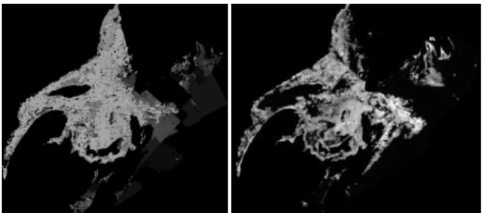
Fig. 8.The texture features used in the ice concentration estimation for 5 March 2009, presented as scaled gray-scale images,Fe(left) andMg(right).

here we useT =10. The reference points are the eight points with the angular step of5/4 around the middle point within a given distanceR; we useR=2. After computing LBP for each pixel location, the minimum of all the cyclic shifts of the eight-bit LBP number is selected to be the final LBP for the pixel; this operation makes the values rotationally invari-ant. These LBP values can then be interpreted as edges (LBP value 15), blunt corners (31) and sharp corners (63). The rela-tive number of edge points within a segment is then the num-ber of the points with the above-mentioned three LBP values (denoted byNe) divided by the area of the segmentA, com-puted in pixels:

Fe=Ne/A. (7)

The other texture feature is based on the three gradient fea-tures, computed in fixed-size, round-shaped (here radiusR= 5) data windows over the SAR image at each image pixel location. The three gradient features basically describe the magnitude and directional coherence of the local image pixel gradient. The gradient texture features are described in detail in (Karvonen, 2012b). Here, we used a combinationMg of the three gradient features:

Mg= q

GF2₁+GF2₂+GF2₃. (8)

This combined gradient featureMgis high in the areas where the SAR signal gradient is high and oriented, i.e. in the areas where the SAR signal is not smooth and there is some kind of non-random structure present. In the concentration algorithm we use segment means of the combined gradient texture fea-ture. An example of the two features used is shown in Fig. 8. As an input for the concentration estimation, we use the maximum of the two texture features, i.e.F =max(Fa, Mg). The concentrationC is estimated with an experimental rela-tionship:

C=   

 

0, ifF < T1, acF, ifT1≤F ≤T2, 100, ifF > T2.

(9)

Here, we have usedT1=10 andT2=30. The thresholds do not have a physical unit; they are related to the SAR texture features. The factorac is defined such thatC is continuous atT1andT2. The thresholdT1andT2were experimentally defined based on visual comparison of six 2003 SAR mosaics and the corresponding CIS ice charts. The fraction of open water (concentration 0 %) can be increased by increasing the value ofT1, and the amount of 100 % concentration ice can be increased by decreasingT2.T1 is smaller than or equal toT2. In the case of equal values for the thresholdsT1 and T2, the algorithm produces only either open water or ice with 100 % concentration.

Open water areas can then simply be found by threshold-ing the concentration. Here, we use 50 % as the threshold. We use this low threshold to make sure all the ice-covered fields are classified as ice, because this discrimination be-tween open water and ice is used as an input for the HIGH-TSI model, and we want to guarantee inclusion of all the ice areas in the HIGHTSI computation.

On the basis of comparison with a visual interpretation of CIS ice charts, the ice concentration estimation seems to work rather well. In general, compared to the CIS ice charts, the concentration was overestimated. We compared the al-gorithm concentrations to CIS ice chart concentrations, ex-tracted as described in Sect. 2, during the period from the beginning of January to the end of March for both the test seasons. The signed mean estimation error, i.e. mean of the CIS ice chart concentration, subtracted from the estimated concentration for this period, was 9.7 percent units for the 2003 data, and 4.4. percent units for the 2009 data set over the same period of the year. During the freeze-up and melting seasons, the overestimation was smaller because the apparent larger open water areas are correctly mapped to the concen-tration of 0 % by the algorithm. During the melting season the algorithm performance is degraded by the wet ice cover and melt ponds, causing underestimation of concentration in these areas. Wet snow cover attenuates the backscattering, and areas of smooth wet snow cover can have SAR signa-tures similar to calm water. Also, large melt ponds have a similar SAR signature as open water. However, according to our experience, the results were not significantly degraded by warm weather conditions, and we were still able to give rea-sonable ice concentration estimates. The main problem for the algorithm seemed to be the overestimation of non-zero concentrations during the mid-winter period.

features from a single SAR measurement, making the esti-mation more robust, especially over open water areas with occasional short (wavelengths in the magnitude of the SAR wavelength) sea wave patterns.

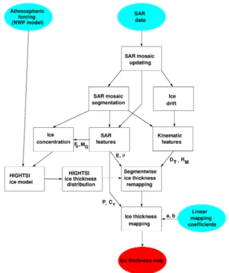
5 SAR- and model-based ice thickness

The correlation between SAR backscattering and different ice types is not always very high (M¨akynen and Hallikainen, 2004; Shokr, 2009); for this reason it is necessary to utilize ice motion and SAR texture features in the ice thickness es-timation. Our ice thickness algorithm utilizes the SAR tures, ice thickness modeled by HIGHTSI, kinematic ice fea-tures (DT,RM) derived from the SAR-based ice drift, and ice concentration from the SAR ice concentration algorithm. A general flow chart of the ice thickness algorithm is presented in Fig. 9. The initial steps of the algorithm are forming and updating the image mosaic. In this process each new SAR image is drawn over the existing mosaic (which in the begin-ning of each season is empty). The mosaic is used as a basis for the daily ice concentration and thickness estimates. The inputs in the diagram are shown in cyan color, and the final output is indicated by red color. The NWP data is received from the ECMWF model; the SAR data is the RADARSAT data from CIS; and the linear mapping coefficients (aandb), used in the final ice thickness estimation phase, are defined based on a training data set, consisting of the 2003 EM mea-surements and SAR mosaic data of the same days with the EM measurements.

To get reasonable estimates of the ice thickness, training data over a representative ice season is required to define the algorithm parameters. Because the season 2002–2003 was more severe with more ice, we selected this season to be the training season, and 2008–2009 to be a test season. Season 2008–2009 could not be used as a training season because it does not cover all the thicker ice cases of the season 2002– 2003. The parameters for ice thickness retrieval were thus defined based on the season 2002–2003 data.

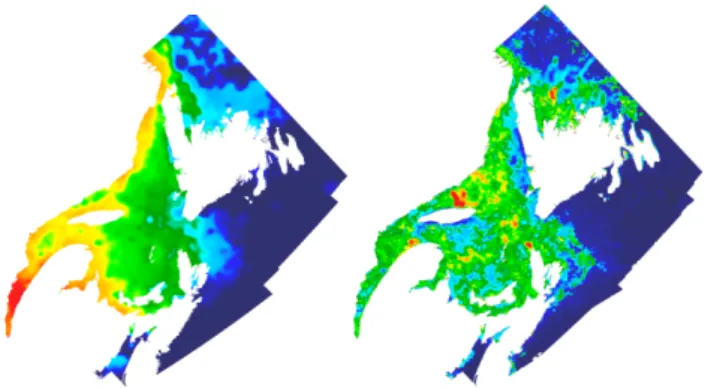
In the next phase, the HIGHTSI ice thickness is remapped based on several segment-wise image features, computed over the SAR mosaics of a period of two weeks before the mosaic of each day. The ice thickness is mapped such that the cumulative feature distribution is mapped to correspond to the HIGHTSI ice thickness distribution computed over the whole study domain. After this mapping computation the SAR feature values in the image grid are mapped to the corre-sponding HIGHTSI ice thickness values according to the cu-mulative distribution matching, i.e. each SAR feature value has a corresponding unique ice thickness value based on the distribution mapping. These statistics represent the cumula-tive ice dynamics during each two-week period. The features computed from the ice motion are the drift ratio RM over the period, total deformationDT, mean SAR pixel valueµ (with incidence angle correction applied) over the period, and

Fig. 9.A general block diagram of the ice thickness estimation scheme. The parameters delivered from one step to another are also shown (with the same names as in the equations).

mean relative amount of edgesE, with respect to the segment area, over the period. The geometric mean of these features is then used to form a new featureF1for each pixel with row and column coordinates(r,c):

Fig. 10.An example of the ice thickness redistribution (5 March 2009, right panel) by matching the HIGHTSI ice thickness (shown in left panel) and the featureF1distributions. The featureF1 in-cludes the kinematic features and SAR texture.

final local ice thickness estimation. This is our background ice thickness grid. An example of this mapping is shown in Fig. 10. This remapped HIGHTSI ice thickness at (r, c) is here denoted byHh(r, c).

Because winds, e.g. winter storms, can cause rather rapid changes in the GSL ice cover (Prinsenberg et al., 2006), the segment-scale background ice thickness field still needs to be refined based on the most recent available local SAR backscattering and texture information in the fine scale (here in 500m mosaic pixel scale). In this final phase of the ice thickness estimation, the segment-scale remapped HIGHTSI ice thickness is used as an input, and it is refined by using the pixel-wise SAR features to get the final local ice thickness es-timates. The basic assumption here is, like for the Baltic Sea ice thickness charts (Karvonen et al., 2003), that the local SAR backscattering and its texture are functions of the ice thickness. In general, it is assumed here that the backscat-tering and the texture at a local scale are stronger for older and thicker ice, which has gone through more deformation events, conditioned by the background ice thickness based on the remapped feature and HIGHTSI distributions. In this final phase the coefficient of variationCv, i.e. the ratio of the local (here the segment-wise) standard deviation and the lo-cal mean (given in percents), is used as an additional texture feature:

Cv(r,c)=100σ (r, c)/µ(r,c), (11) whereµ(r, c)andσ (r, c)are the local mean and standard deviation, respectively, computed for the segment in which the pixel at(r, c)belongs. This feature is also quite robust against variations due to incidence angle. The incidence an-gle corrected SAR pixel value mosaicP (r, c)is modulated byCv(r,c)(geometric mean), and this valueF2(r,c)is used in the fine-scale ice thickness estimation:

F2(r,c)=(Cv(r,c)P (r,c))1/2. (12)

The remapped HIGHTSI ice thickness valuesHh(r, c) are first modulated by the value ofF2, and the ice thicknessH(r, c) at(r, c)is estimated as a linear function of the geometric mean of this modulated term:

H (r,c)=a(Hh(r, c)F2(r,c))1/2+b. (13) We use the valuesa=5.52 andb−112.85 for the linear map-ping parameters. These parameters were defined based on the 2003 EM data (training data set) and the(HhF2)1/2 distribu-tions, using data derived from the same day SAR data with the EM measurements. The distributions were first estimated by smoothing the distributions by a Gaussian kernel with a standard deviation of 10.0. Then the means and standard de-viations for the two distributions (denoted byµ1,µ2,σ1, and σ2) were computed. Assuming, for simplicity, that the distri-butions are Gaussian, we get the mapping coefficients (a and b) between the two distributions:

a=σ2/σ1 and (14)

b=µ2−(σ2/σ1)µ1. (15)

6 Comparisons against CIS ice charts and EM data

6.1 CIS ice charts

The total ice concentrationsCtextracted from CIS ice chart and SAR algorithm for the fifth day of the winter months (January–April) for both ice seasons used in this study are shown in Figs. 11 and 12. The overall agreements are rea-sonably good, although the CIS charts give smaller ice con-centrations in both winter seasons, particularly in February and April. In each February and April, the difference for the cold winter (2002–2003) is slightly higher compared with results for the milder winter (2008–2009). However, because the distinction between ice and open water is based on the ice concentration algorithm output, and this result is used as an input for HIGHTSI, we rather slightly overestimate the con-centration to include all the ice-covered areas in the HIGH-TSI computation than leave ice-covered areas out of the com-putation. The difference in the mid-winter (January–March) was from 4.4 (2009) to 9.6 percentage points, the overall L1 (absolute mean error) was 15.9 (2003) and 13.9 percentage points.

(a) (b)

(c) (d)

(e) (f)

(g) (h)

Fig. 11.Ice concentrations for the 5 January(a–b), 5 February(c– d), 5 March(e–f), and 5 April(g–h)2003 from the CIS ice charts (left column) and based on our SAR algorithm (right column).

because the ice thickness ranges of the degree of develop-ment categories are wide and usually overlap each other. This crude analysis also contributed to differences between CIS-and SAR-based ice thickness. The ice drift was estimated in a resolution of 8 km (corresponding to the window size of the ice motion estimation algorithm, multiplied by the SAR mo-saic resolution, i.e. 16×500 m); in this scale the motion in narrow straits and river outflows cannot be detected, and the HIGHTSI remapping in these areas fails. This could proba-bly be improved by estimating the motion in a higher reso-lution (we have used the 500 m mosaic resoreso-lution). On the other hand, there are similarities between CIS- and SAR-based ice thickness, particularly in terms of ice thickness distributions. The distributions for the area where the annual EM measurements have been made match each other rather well. For the areas with larger deviations between the CIS ice charts and the thickness estimates, the differences can be

(a) (b)

(c) (d)

(e) (f)

(g) (h)

Fig. 12.Ice concentrations for the 5 January(a–b), 5 February(c– d), 5 March(e–f), and 5 April(g–h)2009 from the CIS ice charts (left column) and based on our SAR algorithm (right column).

due to failure of our algorithm to capture all the ice motion, misinterpretation of the SAR features by our algorithm, or by the coarse presentation in the CIS ice charts.

The ice thickness distributions from HIGHTSI represent the thermodynamic ice growth, and considerably differ from distributions based on the CIS ice charts. Because HIGHTSI literally produces the basin-scale thermodynamic ice growth, the effect of ice dynamics such as ice deformation, rafting, and ridging are not included. On the other hand, the basin-scale sea ice production agreed reasonable well compared with CIS data (Fig. 5).

(a) (b) (c)

(d) (e) (f)

(g) (h) (i)

(j) (k) (l)

Fig. 13.Ice thickness for the 5 January(a–c), 5 February(d–f), 5 March(g–i), and 5 April(j–l)2003 from the CIS ice charts (left column), from HIGHTSI model (middle column), and based on the SAR algorithm (right column).

that the training of the algorithm, i.e. definition of the linear mapping parameters a andb, has been performed only on the basis of the short period of EM measurements from 27 February to 4 March 2003 over a limited area close and be-tween the Magdalen Islands and Prince Edward Island. With a temporally and spatially more representative training data set, better results could be reached.

In general, we can say that the CIS ice charts give a useful reference for comparing the ice concentration; the ice thick-ness is only a rough first order estimate, but it can at least be used in qualitative visual comparison. Ice concentration has a different nature than ice thickness, because it is a quantity relative to the segment area, and reasonable values to large segments can always be given. However, because no other ice thickness measurements covering large spatial and temporal

(a) (b) (c)

(d) (e) (f)

(g) (h) (i)

(j) (k) (l)

Fig. 14.Ice thickness for the 5 January(a–c), 5 February(d–f), 5 March(g–i), and 5 April(j–l)2009 from the CIS ice charts (left column), from HIGHTSI model (middle column), and based on the SAR algorithm (right column).

the limited training of the algorithm; the CIS ice charts could not be used as a training data set because of the coarse reso-lution and the ambiguities in the ice thickness extracted).

A systemic evaluation of CIS- and SAR-based ice thick-ness charts reveals that the correspondence between the SAR ice thickness products and the CIS ice charts for the winter 2002–2003 is better than for 2008–2009. This also applies to the other shown examples (not only to March 2003, which includes some of the training data points). For example, in February 2009 the thick ice area visible in the ice chart north of Prince Edward Island was not detected by the algorithm, and the ice thickness was underestimated. On the other hand, there are smaller, thicker ice segments in the thick ice area based on our algorithm, and also small very thin ice areas. It is impossible to say which interpretation actually corre-sponds the truth. Further, some areas of thicker and thinner ice are found from different locations, for example in March 2003 (Fig. 13g and h) the thin and thick ice are on different sides of the strait of Belle Isle (separating Labrador penin-sula from Newfoundland) in the northern part of GSL, in the ice chart and ice thickness estimate by our algorithm. Such estimation errors can be due to some rapid strong ice motions which have not been detected by the ice drift estimation algo-rithm. Such errors can only be corrected by having a higher temporal resolution to enable continuous tracking of the ice drift.

6.2 EM measurements

The EM measurements were acquired during the relatively short time periods in late February and early March for both ice seasons studied, as described in Sect. 2.

EM ice thickness measurements essentially include the snow thickness. Unfortunately we did not have any statistics on the snow cover over GSL sea ice. Typically, snow cover over sea ice is not very thick in Northern Hemisphere. HIGH-TSI modeled basin-scale mean snow thickness was roughly 8 % and 20 % of the total mean ice thickness over the winter seasons 2002–2003 and 2008–2009, respectively. Statistical analysis suggests that for ice thicker than 20 cm, the snow thickness is roughly 9–10 % of the ice thickness over Arctic sea ice (Doronin, 1971; M¨akynen et al., 2012). We, therefore, decided not to make any snow corrections for the EM data, i.e. the EM thicknesses used in this study are thus slightly biased by the snow thickness. On the other hand, as we have used the EM data with the snow cover included in the train-ing of the algorithm, the snow cover is also included in the thickness estimates.

The ice thickness values were compared to EM thickness measurements made in the GSL in 2003 and 2009. Applying a sliding median window along the EM measurement line, the EM measurements were smoothed to a resolution simi-lar to that of the SAR data mosaics (500 m). The combined comparisons along all the EM measurement lines are shown in Fig. 15. In the figure the algorithm thickness estimates at

Table 3.Kolmogorov–Smirnov statistics compared to the EM ice thickness.

Season SAR algor. HIGHTSI CIS IC

2002–2003 0.194 0.646 0.347

2008–2009 0.180 0.624 0.675

each resampled (to the algorithm resolution) EM measure-ment point are shown with the resampled EM measuremeasure-ment values, the CIS ice chart ice thickness, and the ice thickness given by HIGHTSI.

The EM data from 2009 are independent, but the 2003 data were used for defining the mapping coefficients from the SAR features and HIGHTSI results to the ice thickness estimates. In general, the SAR algorithm overestimates the ice thickness; for the test data of 2009 the mean overestima-tion was 11.4 cm, and for the 2003 data 2.7 cm. It also seems that there are some shifts between the EM measurements and SAR thickness estimates. This is probably due to the ice mo-tion and temporal differences (the mosaics contain data from multiple SAR images with different acquisition times) be-tween the EM measurement and the SAR acquisition. Reg-istration inaccuracies between the EM and SAR mosaic data sets are also possible. Assuming the EM measurements are precisely geocoded, the possible registration errors are made in making the mosaic based on the SAR geocoding, which may contain inaccuracies.

Because it seems that direct pixel-wise comparison does not give very convincing error statistics (due to the above-mentioned shifts), we also compared the ice thickness distri-butions based on the SAR algorithm, CIS ice charts, HIGH-TSI experiments, and EM measurements. The comparison was limited to the EM measurement lines. We computed the Kolmogorov–Smirnov statistics between the EM ice thick-ness distribution, the CIS ice chart mean ice thickthick-ness, and the HIGHTSI ice thickness. The Kolmogorov–Smirnov statisticsDn between two cumulative distribution functions Fn(x)andF (x)is

Dn=supx|Fn(x)−F (x)|, (16) where the cumulative distributions are also functions of the ice thickness. The Kolmogorov–Smirnov statistics are tabu-lated in Table 3, the mean ice thickness along the EM flight lines are tabulated in Table 4, and the comparison of the ice thickness distributions is shown in Fig. 16.

Fig. 15.The ice SAR algorithm thickness compared to HIGHTSI ice thickness, mean ice thickness derived from digitized CIS ice charts, and EM ice thickness measurements along the EM measurement lines for the two test seasons (2002–2003 in left panel, 2008–2009 in right panel). The x-axis value is the number of the EM measurements resampled to the SAR mosaic resolution of 500 m; in the figure all the EM flight lines for each year have been concatenated in temporal order.

Fig. 16.The ice thickness distributions from different sources along the EM measurement lines for both the test seasons, 2002–2003 on the left and 2008–2009 one the right.

Table 4.Mean ice thickness (in cm) according to different sources along the EM flight lines for the two seasons.

Source 2002–2003 2008–2009

SAR algor. 52.0 59.1

CIS IC 15.2 18.8

HIGHTSI 40.4 23.1

EM 49.3 47.7

2002–2003 (Table 4). The mean overestimation for 2002– 2003 was only 5.5 %, and 23.9 % for 2008–2009, compared to the EM measurements. As the 2008–2009 data are inde-pendent, and 2002–2003 data have been used in training of the algorithm, a larger error for the 2008–2009 data was ex-pectable.

7 Conclusions

We developed a novel methodology for deriving sea ice pa-rameters based on a thermodynamic ice model and SAR data in a fully automated manner over GSL. Our algorithms pro-duce ice concentration and thickness estimations utilizing in-put data from a thermodynamic ice model, SAR-based ice motion, and SAR texture features. The method has been ap-plied for GSL with promising results.

The HIGHTSI-based ice thickness is only affected by ther-modynamic growth and melt. Ice dynamics was considered by incorporating ice concentration information from SAR data analysis. In the basin scale, the modeled evolution of ice thickness was comparable with that based on the CIS ice charts. The results suggested that the seasonal evolution of ice thickness and area are largely dominated by the weather forcing conditions. The main sources of uncertainty in the model experiments were the amount of snow fall and the oceanic heat flux.

the same area with a reasonable temporal difference, the ice concentration estimates can be further improved by using a temporal minimum (or some other temporal filtering) over a short time period. Using a temporal minimum would reduce the overestimation compared to CIS ice charts, but also, for example, temporal mean or median could be used instead. The reasonable temporal difference depends on the prevail-ing ice conditions; in the freezprevail-ing and meltprevail-ing periods with rapid changes, it could be about one day, and in the mid-season even several days. Recently, posterior to this study, a more advanced method for ice concentration estimation from C-band HH-channel SAR data has been developed (Karvo-nen, 2012c), and applying this method would probably im-prove the ice concentrations estimates.

The ice thickness estimation also produced promising re-sults: validation against the local EM measurements showed that the ice thickness based on the new method was much more realistic than that based on the CIS ice charts. A prob-lem in SAR-based ice thickness estimation is, however, to locate areas of thin ice. SAR backscattering and texture for deformed thin ice is sometimes very similar to the values for deformed thick ice areas. We have tried to address this prob-lem by utilizing the ice drift from SAR data together with the thermodynamic ice model. However, the coarse resolution of the ice drift used here cannot yield proper ice drift informa-tion over narrow sea areas (straits) present in GSL. Also, the temporal resolution of SAR data at a given location varies from half a day to several days, and thus the SAR-based ice drift can only yield reliable statistics over periods of a few weeks. Rapid dynamic events can currently only be detected on the basis of SAR texture interpretation. It has been shown that radiometer data can be used for estimation of the thin ice thickness (Yu and Rothrock, 1996; Kaleschke et al., 2010; M¨akynen et al., 2010), and combining this information with the SAR data would be useful in better estimation of the thin ice thickness.

The ice thickness in the CIS ice charts is based on the stage of development, and it does not provide very good quantita-tive reference values. The CIS ice chart concentration seems to be a more reasonable reference for our new products. However, the CIS ice chart thicknesses at least give some idea of large-scale spatial variations in the ice thickness. Be-cause of the coarse nature of the ice thickness description of CIS ice charts (large polygons, and large ice thickness ranges within each polygon) local ice thickness at the resolution of the SAR algorithm is, however, not well described in the ice charts. This fundamental difference also partly explains dif-ferences between the SAR algorithm results and the CIS ice charts. Comparisons to ice thickness distributions from re-sampled EM data and SAR algorithm produced relatively good results, but the results for single point measurements were not good because there seemed to be shifts between the ice thickness estimates and EM values along the flight lines. These shifts are mainly due to temporal differences between

the SAR acquisition time at each SAR mosaic grid location and the corresponding EM measurements.

An alternative approach would be to make the ice analysis on the basis of observations and a dynamic–thermodynamic model. Modeling of ice dynamics in a complex coastal or archipelago region is, however, very challenging (Gao et al., 2011). The coarse resolution of the models also involves the problem that ice drift in narrow straits cannot be properly modeled. Our method is, however, not affected by the error sources of modeling sea ice dynamics.

Our estimates are directly affected by the temporal res-olution of the SAR data. Because in the SAR mosaics we always use the most recent SAR data, poor temporal resolu-tion may sometimes cause the problem that data over some areas is several days old, and not well representative for the current ice conditions. Sparse temporal data also affect the ice drift estimation, and with too sparse temporal coverage some ice dynamics may not be captured by the algorithm. In the near future satellite constellations, like the X-band Ital-ian COSMO-SkyMed (already in operation), ESA’s C-band Sentinel-1 (estimated launch 2013), and Canadian C-band RADARSAT constellation (estimated launch 2015), will pro-vide better temporal coverage, and result in an improved SAR-derived product quality via improved ice drift detection and faster updating of mosaics.

In our opinion the SAR ice thickness estimation algorithm has potential for operational use. The main challenge towards operational sea ice thickness estimation is probably the lack of in-situ measurements for proper algorithm calibration and validation. To build a reliable operational system, almost si-multaneous in-situ data with the SAR acquisition (delay no more than a few hours) throughout the ice season would be required for calibration and validation of an algorithm. In this study we only had EM measurements over a short temporal period for both study seasons, and also the spatial coverage of the EM data was limited. For this reason we have also tried to make some quantitative comparison to the ice information extracted from the CIS ice charts. Typically, in-situ measure-ments are collected in campaigns with a limited spatial and temporal coverage. For development of improved EO algo-rithms and numerical models, systematic collection of refer-ence sea ice data with a representative temporal and spatial coverage would be desirable.

In the future the algorithm can be improved by computing the ice motion in a finer spatial and temporal scale, taking into account smaller details (narrow straits and river inflows). Also, incorporating data from other EO sources for improved thin ice identification will be considered. The algorithms will also be applied for other ice-covered seas, with validation against available observations.

methodology that could be used for automated sea ice in-formation retrieval, presuming a high enough SAR data ac-quisition frequency to produce continuous ice drift estimates and more frequent SAR mosaic updates. With the current SAR acquisition frequency, the mosaic data in some areas are older than one day, even several days. In practice, the SAR data should cover the whole area daily to get reliable ice parameter estimates.

Some current (RADARSAT-2) and forthcoming SAR mis-sions (Sentinel-1 and RADARSAT constellations) also have the possibility to acquire dual-polarized data, i.e. both co-polarized (either HH or VV polarization combination) and cross-polarized channels (HV or VH) can be acquired simul-taneously. Using cross-polarized SAR data, containing com-plementary information in addition to the co-polarized SAR data, can improve the sea ice classification, especially in lo-cating open water, thin ice, and deformed ice areas (Scheuchl et al., 2004; Geldsetzer and Yackel, 2009). Utilization of dual-polarized SAR data in our algorithms would produce improved ice concentration and ice thickness estimates. De-velopment and evaluation of an ice thickness estimation algo-rithm based on polarized SAR data would require dual-polarized SAR data from at least one whole ice season over the area of interest. The major advance of the forthcoming SAR constellations will, however, be that the temporal cov-erage will be considerably improved as the planned multiple SAR constellations will be realized. Their realization will ac-complish the objective of covering the Arctic waters daily at a high resolution.

Acknowledgements. The Gulf of Saint Lawrence experiment was funded and the Canadian NWP data were provided by Environment Canada.

The EM ice thickness data was provided by Fisheries and Oceans Canada.

RADARSAT-2 data and products (season 2008–2009)

©MacDonald, Detweiler and Associates Ltd. (2008) – All rights Reserved.

RADARSAT-1 data and products (season 2002–2003) ©Canadian Space Agency.

ECMWF is acknowledged for providing us the NWP model results.

The work of Timo Vihma was supported by the Academy of Finland (contract 259537).

Edited by: D. Feltham

References

Andersen, S., Tonboe, R., Kaleschke, L., and Heygster, G.: Inter-comparison of passive microwave sea ice concentration retrievals over the high-concentration Arctic sea ice, J. Geophys. Res., 112, C08004, doi:10.1029/2006JC003543, 2007.

Astola, J., Haavisto, P., and Neuvo, Y.: Vector median filters, P. IEEE, 78, 678–689, 1990.

Biazzi, B., Alparone, L., Baronti, S., and Borri, G.: Pyramid-based multi-resolution adaptive filters for additive and multiplicative image noise, IEEE T. Circuits-II, 45, 1092–1097, 1998. Bitz, C. M., Holland, M. M., Weaver, A. J., and Eby, M.:

Simulat-ing the ice-thickness distribution in a coupled climate model, J. Geophys. Res., 106, 2441–2464, 2001.

Briegleb, B. P., Bitz, C. M., Hunke, E. C., Lipscomb, W. H., Hol-land, M. M., Schramm, J. L., and Moritz, R. E.: Scientific de-scription of the sea ice component in the Community Climate System Model, Version Three. Tech. Rep. NCAR/TN-463+STR, National Center for Atmospheric Research, Boulder, CO, 78 pp., 2004.

Bromwich, D. H., Hines, K. M., and Bai, L.-S.: Develop-ment and testing of polar weather research and forecast-ing model: 2. Arctic Ocean, J. Geophys. Res., 114, D08122, doi:10.1029/2008JD010300, 2009.

Canny, J.: A computational approach to edge detection, IEEE T. Pattern Anal., 8, 679–698, 1986.

Cheng, B., Vihma, T., and Launiainen, J.: Modelling of the super-imposed ice formation and sub-surface melting in the Baltic Sea, Geophysica, 39, 31–50, 2003.

Cheng, B., Vihma, T., Pirazzini, R., and Granskog, M.: Modelling of superimposed ice formation during spring snow-melt period in the Baltic Sea, Ann. Glaciol, 44, 139–146, 2006.

Cheng, B., Zhang, Z., Vihma, T., Johansson, M., Bian, L., Li, Z., and Wu, H.: Model experiments on snow and ice thermodynamics in the Arctic Ocean with CHINAREN 2003 data, J. Geophys. Res. 113, C09020, doi:10.1029/2007JC004654, 2008a.

Cheng, B., Vihma, T., Zhang, Z., Li, Z., and Wu, H.: Snow and sea ice thermodynamics in the Arctic: model validation and sensitiv-ity study against SHEBA data, Chinese Journal of Polar Science, 19, 108–122, 2008b.

DeGroot, M. H.: Probability and Statistics, 3rd Edn., Addison-Wesley, Boston, 1991.

Doronin, Y. P.: Thermal interaction of the atmosphere and the hy-drosphere in the arctic, Coronet Books, ISBN 0706510372 (0-7065-1037-2), 1971.

Ebert, E. E. and Curry, J. A.: An Intermediate one-dimensional ther-modynamic sea ice model for investigating ice-atmosphere inter-action, J. Geophys. Res., 98, 10085–10109, 1993.

Fichefet, T. and Maqueda, M. A. M.: Sensitivity of a global sea ice model to the treatment of ice thermodynamics and dynamics, J. Geophys. Res., 102, 609–646, doi:10.1029/97JC00480, 1997. Flato, G. M. and Brown, R. D.: Variability and climate sensitivity

of landfast Arctic sea ice, J. Geophys. Res., 101, 25767–25777, 1996.

Gabison, R.: A thermodynamic model of the formation growth and decay of first-year sea ice, J. Glaciol., 33, 105–109, 1987. Gao, G., Chen, C., Qi, J., and Beardsley, R. C.: An