www.the-cryosphere.net/10/1529/2016/ doi:10.5194/tc-10-1529-2016
© Author(s) 2016. CC Attribution 3.0 License.
Retrieval of the thickness of undeformed sea ice from
simulated C-band compact polarimetric SAR images
Xi Zhang1, Wolfgang Dierking2, Jie Zhang1, Junmin Meng1, and Haitao Lang3 1The First Institute of Oceanography, State Oceanic Administration, Qingdao, China 2Alfred Wegener Institute for Polar and Marine Research, Bremerhaven, Germany 3Beijing University of Chemical Technology, Beijing, China
Correspondence to:Xi Zhang ([email protected]) and Haitao Lang ([email protected]) Received: 29 August 2015 – Published in The Cryosphere Discuss.: 15 October 2015
Revised: 9 June 2016 – Accepted: 23 June 2016 – Published: 19 July 2016
Abstract.In this paper we introduce a parameter for the re-trieval of the thickness of undeformed first-year sea ice that is specifically adapted to compact polarimetric (CP) syn-thetic aperture radar (SAR) images. The parameter is de-noted as the “CP ratio”. In model simulations we investigated the sensitivity of the CP ratio to the dielectric constant, ice thickness, ice surface roughness, and radar incidence angle. From the results of the simulations we deduced optimal sea ice conditions and radar incidence angles for the ice thick-ness retrieval. C-band SAR data acquired over the Labrador Sea in circular transmit and linear receive (CTLR) mode were generated from RADARSAT-2 quad-polarization im-ages. In comparison with results from helicopter-borne mea-surements, we tested different empirical equations for the re-trieval of ice thickness. An exponential fit between the CP ra-tio and ice thickness provides the most reliable results. Based on a validation using other compact polarimetric SAR im-ages from the same region, we found a root mean square (rms) error of 8 cm and a maximum correlation coefficient of 0.94 for the retrieval procedure when applying it to level ice between 0.1 and 0.8 m thick.
1 Introduction
Sea ice covers about one-tenth of the world ocean surface and significantly affects the exchanges of momentum, heat, and mass between the sea and the atmosphere. Not only is sea ice extent a significant indicator and effective modulator of regional and global climate change, but sea ice thickness is also an important parameter from a thermodynamic and
kine-matic perspective (Soulis et al., 1989; Kwok, 2010). The de-cline of sea ice extent recently observed in the Arctic, e.g., is linked with a decrease of ice thickness and increasing frac-tions of seasonal ice areas (e.g., Kwok et al., 2009). Measure-ments of sea ice thickness are compared with model results to control and validate the model capabilities of reproducing recent and predicting future trends of sea ice conditions in the Arctic (e.g., Laxon et al., 2013). Although sea ice thickness is only several meters at most, it forms an effective thermal insulation layer due to its high albedo and low thermal con-ductivity, leading to a significant reduction in the heat flux from the ocean to the atmosphere, especially in winter (Van-coppenolle et al., 2005). Besides investigations focusing on the entire Arctic or Antarctic region, other studies analyze ice thickness variations on local scales to improve regional ice thickness retrievals (e.g., Haapala et al., 2013). Operational services charged with providing sea ice maps and forecast-ing ice conditions for marine transportation and offshore op-erations need near-real-time regular information about local and regional ice thickness distributions. The use of sensors providing high spatial resolutions on the order of 100 m or better for ice thickness retrieval, such as synthetic aperture radar (SAR), is an important topic of recent research (Dierk-ing, 2013).
thickness distributions at larger spatial scales, remote sens-ing methods are requisite tools. There are generally different strategies.
1. Measurements of ice draft using upward-looking sonar on ocean moorings or submarines (Wadhams, 1980; Behrendt et al., 2013) from which thickness is estimated based on assumptions about buoyancy, ice density, and snow load (e.g., Rothrock et al., 1999) are used. Such data provide information about detailed temporal thick-ness variations (daily or even hourly) at a fixed loca-tion. An example for using in situ measurements of ice thickness from the New Arctic Program initiated by the Canadian Ice Service (CIS) starting in 2002, and sea ice draft measurements from moored upward-looking sonar (ULS) instruments in the Beaufort Gyre Observing Sys-tem for testing a method of ice thickness retrieval from optical methods is provided by Wang et al. (2010). 2. Measurements of sea ice freeboard (i.e., the part of the
ice above the water level) plus snow layer thickness with laser altimetry (e.g., Wadhams et al., 1992; Dierking, 1995) are used. From such data, the average ice thick-ness can be estimated, or the probability density func-tion (PDF) of ice freeboard can be converted to a PDF of ice thickness. However, the estimation of ice thick-ness from freeboard data is less reliable than from ice draft because of a relatively stronger impact of errors in the freeboard measurements (Goebell, 2011).
3. The distance between snow surface and ice bot-tom is measured with electromagnetic induction sounders (EMSs) mounted on sledges, ships, or he-licopters/airplanes (Goebell, 2011; Haas et al., 1997; Prinsenberg et al., 2012a, b). With such systems, spa-tial ice thickness variations measured at horizontal dis-tances of a few 10 m were obtained in various regions (Kovacs et al., 1987; Rossiter and Holladay, 1994; Haas et al., 2006; Hendricks et al., 2011).
Although ULSs and EMSs have all contributed greatly to our knowledge about ice thickness distributions on local and re-gional scales, such data can only be obtained at specific loca-tions over a limited time period. Satellite remote sensing, on the other hand, is useful to monitor ice thickness variations regularly over much larger areas.
On a still experimental basis, data of L-band passive mi-crowave sensors, such as for example the Soil Moisture and Ocean Salinity mission (SMOS) radiometer, have been em-ployed to retrieve thickness of sea ice thinner than about 0.5 m. The limitation of this approach is that it is only pos-sible for very high (almost 100 %) sea ice concentration and in cold freezing conditions (Tian-Kunze et al., 2014; Hunte-mann et al., 2014). A space-borne altimeter has been used primarily to map ice thickness, and to monitor and study trends in thickness changes. The capabilities of laser and
radar altimeter systems (such as CryoSat-2 and ICESAT) of measuring ice freeboard have been extensively investigated during the last decade (e.g., Kwok and Cunningham, 2008; Kwok et al., 2009; Laxon et al., 2013). Compared with ra-diometers, which only collect data at a coarse spatial resolu-tion of a few to tens of kilometers (e.g., 25 km for the Special Sensor Microwave Imager (SSM/I) 37 GHz data), the spatial resolutions of radar altimeter systems are about 250 m along-track and 1.5 km across-along-track for CryoSat-2, and the foot-print for ICESAT is about 70 m diameter. The sea ice prod-ucts derived from altimeters usually focus on large-scale spa-tial and temporal variations. While the large-scale ice thick-ness product is important for climate research, the support of marine navigation and offshore operations in polar areas are crucially dependent on precise and reliable sea ice thickness maps with spatial resolutions better than 1 km.
Space-borne synthetic aperture radar (SAR), which oper-ates in the microwave frequency band, provides all-weather and day–night high-resolution imagery (within a range of 1–100 m) with 1–3 days’ temporal coverage. Hence, SAR is in general very useful for operational mapping tasks on regional and local spatial scales (Dierking, 2013). The dis-advantage of SAR systems is that higher spatial resolutions are linked with a limited coverage between 10 and 500 km, compared, for example, to more than 1000 km for passive microwave radiometers. SAR measures the intensity of the radar signal backscattered from the ice surface and volume at different polarizations. The backscattered intensity depends on the dielectric constant of the ice and small-scale (mm– dm range) ice properties such as ice surface roughness and air bubble fractions and sizes. If at least two polarizations are measured simultaneously, the SAR, which is a coher-ent device, can also provide the phase difference between the differently polarized channels. The most recent SAR sen-sors have polarimetric capabilities. A fully polarimetric radar transmits and receives both linear horizontal (H) and ver-tical (V) polarized electromagnetic waves. Amplitude and phase information of the backscattered signal are recorded for four transmit/receive polarizations (HH, HV, VH, and VV). This mode is commonly referred to as “quad-pol”. Quad-pol scenes are usually acquired at very high spatial olution. A RADARSAT-2 quad-pol scene has a spatial res-olution of 4.7 m (slant range)×5.0 m (azimuth) at a swath width of 25/50 km. Dual-pol scenes contain two polarimetric channels (e.g., HH and HV or VV and VH). In operational ice-charting services, dual-pol scenes are preferred because of their wider areal coverage (Geldsetzer et al., 2015). The RADARSAT-2 ScanSAR wide mode, e.g., can have a swath width of 500 km with 160–72 m (ground range)×100 m (az-imuth) resolution. Despite their currently very limited cover-age, the quad-pol images are important information sources to understand the scattering mechanisms of sea ice.
we use VV / HH). The sensitivity between co-polarization ratio and thin ice thickness was first demonstrated by On-stott (1992), based on C-band radar data from the eastern Arctic region. Kwok et al. (1995) estimated the thin ice thick-ness (0 to 0.1 m) from L- and C-band fully polarimetric air-borne SAR data acquired over the Beaufort Sea. Their ap-proach included the training of a neural network. L-band po-larimetric characteristics of ice in the Sea of Okhotsk were investigated by Wakabayashi et al. (2004), and the L-band co-polarized ratio was used to estimate ice thicknesses be-tween 0 and 2 m (their Fig. 13). The investigation was fur-ther extended to ofur-ther sensors, e.g., to the airborne Pi-SAR (X- and L-band data from the Sea of Okhotsk; Nakamura et al., 2009a; Toyota et al., 2009) and to Envisat ASAR, us-ing radar intensity and ice thickness data from 0.2 to 2.5 m, the latter acquired from a research vessel in Lützow-Holm Bay, Antarctica (Nakamura et al., 2009b). The good correla-tions were attributed to the fact that the co-polarized ratio val-ues are sensitive to the dielectric constants of the ice surface layer which change due to the process of desalination during ice growth. The relationship between relatively thick multi-year ice (thickness between 2 and 5 m), on the one hand, and co-polarized correlation and cross-polarized ratio HV/HH or VH/VV, on the other hand, was also investigated in the Arc-tic Ocean employing RADARSAT-2 and TerraSAR-X data (Kim et al., 2012). They found that the degree of depolar-ization is linked to the thickness of the multi-year ice as ice surface roughness increases and salinity decreases.
Although the above-mentioned parameters derived from polarimetric SAR imagery have shown the potential for esti-mating sea ice thickness under certain conditions, polarimet-ric SAR data can presently only be acquired at limited swath-widths. The quad-pol mode on RADARSAT-2 has a swath width of only 25–50 km, as mentioned above. The swath width of the VV/HH dual-polarization StripMap mode on TerraSAR-X is 15 km. Therefore, they are insufficient for op-erational use which requires a large-scale coverage (Scheuchl et al., 2004). The limited swath width also restricts scientific investigations to local domains. An alternative is to use com-pact polarimetry.
The methods of generating compact polarimetric (CP) in-formation (explained below) are based on receiving data at two different polarizations (Souyris et al., 2005; Raney, 2007). Compared with the “traditional” dual-polarization modes described above, CP data include a greater amount of polarization information (but less than quad-polarization data). They can cover much greater swath widths compared to quad-polarization modes due to reduced power consump-tion and data storage requirements.
The term “CP system” refers to a unique polarization in transmission and coherent dual-orthogonal polarizations in reception. There are three different CP configurations (Nord et al., 2009). The first one is theπ/4 mode, with a slant lin-ear transmission and horizontal (H) and vertical (V) recep-tions (Souyris et al., 2005). The second is the dual
circu-lar (DC) mode, i.e., transmitting at a single circucircu-lar pocircu-lar- polar-ization and receiving two orthogonal circular polarpolar-izations. The last approach is circular transmit and linear (H and V) receive (called CTLR mode). Among these three com-pact polarization modes, the latter has been ranked to be the most promising in terms of performance and receiver com-plexity. The current Indian RISAT-1, the Japanese ALOS-2, and the planned Canadian RADARSAT Constellation Mis-sion (RCM) also support the CTLR mode. According to the description in Geldsetzer et al. (2015), the coming CTLR mode of RCM will be particularly tailored to sea ice appli-cations by offering a medium-resolution mode with a swath width of 350 km and a resolution of 50 m, a low-noise mode with the same swath width and a resolution of 100 m, or a low-resolution mode with a swath width of 500 km and a res-olution of 100 m. Hence, the CTLR modes of RCM are well suited for operational sea ice monitoring.
However, one apparent disadvantage of the CP mode as compared to dual- or quad-polarization mode is the fact that the HH, VV, and HV signal combinations are not directly measured. This means that the co-polarized ratio (Wak-abayashi et al., 2004; Nakamura et al., 2009a; Toyota et al., 2009) and the cross-polarized ratio (Kim et al., 2012) which are often used as an ice thickness proxy cannot be directly calculated from CP-mode SAR data. Although CP SAR im-ages have been used to distinguish sea ice types (Dabboor and Geldsetzer, 2014; Charbonneau et al., 2010; Geldsetzer et al., 2015), to our knowledge there have been no published studies on its use for ice thickness detection in the open lit-erature until now. Therefore, in this study, we considered the CTLR mode and developed an approach to directly retrieve the thickness from CP SAR data (hereafter we assume that the CP SAR is operated in CTLR mode). The paper is or-ganized as follows: in Sect. 2 we introduce a new parameter to estimate ice thickness and demonstrate its sensitivity to different ice parameters by numerical modeling in Sect. 3. In Sect. 4, an empirical relationship based on a comparison of CP-SAR signatures with ice thickness data obtained from electromagnetic induction sounding is presented, and the re-trieval performance of this algorithm is described. Further discussions and conclusions are presented in Sect. 5.
2 Model and method
2.1 Full polarimetry and compact polarimetry
The full polarimetric radar scattering return can be repre-sented by the scattering matrixS:
S=
SHH SHV SVH SVV
, (1)
We use the coherency matrixTto evaluate the second-order statistics of the scattering matrixS. The coherency matrixT formed from the elements of the scattering matrixSis T=1
2
|SHH+SVV|2 (SHH+SVV) (SHH−SVV)∗ 2(SHH+SVV) S∗HV
(SHH−SVV) (SHH+SVV)∗ |SHH−SVV|2 2(SHH−SVV) S∗HV
2
SHV(SHH+SVV)∗ 2SHV(SHH−SVV)∗ 4|SHV|2 , (2) where∗ denotes the complex conjugate andh idenotes the
ensemble average.
We consider the CTLR mode for which the scattering vec-tors are given by (e.g., Nord et al., 2009)
kCTLR=[SRHSRV]T =[SHH−iSHV−iSVV+SHV]T/√2. (3)
As usual, R denotes that the transmitted polarization is right circular, while H and V stand for the linear reception. We set 6H=SRH+iSRV 6V=SRH−iSRV. (4) From Eq. (3) it then follows that
6H=SHH+SVV6V=SHH−SVV−i2SHV. (5) The termsh|6H|2iandh|6V|2ican be expressed as
D
|6H|2 E
=
(SHH+SVV) (SHH+SVV)∗
=D|SHH+SVV|2 E
,
D
|6V|2 E
=(SHH−SVV−i2SHV) (SHH−SVV−i2SHV)∗
=(SHH−SVV) (SHH−SVV)∗+i2SHV∗ (SHH
−SVV)i −
i2SHV(SHH−SVV)∗
+4|SHV|2
=
D
|SHH−SVV|2 E
+i2SHV∗ (SHH−SVV)
−i2SHV(SHH−SVV)∗
+4|SHV|2. (6) Under the assumption of reflection symmetry, the cross- and co-polarized scattering coefficients are uncorrelated. This as-sumption is reasonable for snow and sea ice surfaces at var-ious frequencies and for different spatial scales (Souyris et al., 2005). Hence
SHV∗ SVV=SHHSHV∗ ≈0, (7) and Eq. (6) can be rewritten by the elements of coherency matrixT:
D
|6H|2 E
=D|SHH+SVV|2 E
=t11 D
|6V|2 E
=D|SHH−SVV|2 E
+4|SHV|2=t22+t33. (8)
2.2 X-Bragg model and X-SPM model
According to the results obtained by the Cold Region Re-search and Engineering Laboratory (CRREL’88), the typi-cal ranges of root mean square (rms) height and correla-tion lengths for smooth level sea ice are 0.02–0.143 and 0.669–1.77 cm respectively (Fung, 1994). For C-band SAR, the small perturbation method (SPM) can be applied for ex-plaining the surface scattering characteristics from smooth level sea ice. By doing so, the underlying assumption is that the received radar signatures are typical for Bragg scattering. However, the SPM fails to describe cross-polarization and de-polarization effects that are observed in real SAR data. In order to overcome these limitations and to widen the SPM range of validity, an extended Bragg model (termed X-Bragg model) was presented by Hajnsek et al. (2003). In the X-Bragg model, the scattering surface is composed of rough randomly tilted facets that are large with respect to the wave-length but small with respect to the spatial resolution of the sensor (for RADARSAT-2 fine-quad mode, the wavelength is 5.6 cm and the resolution is 8 or 25 m). Scattering from each rough facet is evaluated by employing the SPM, whereby for the facets, a random tilt is assumed which causes both a ran-dom variation1θof the incidence angleθand a random rota-tionβof the local incidence plane around the line of sight. In the X-Bragg model, the random incidence angle variation1θ is ignored, and the incidence plane angle of rotationβ is as-sumed to be uniformly distributed in an interval (−β1,β1), where the parameterβ1is used to characterize the large-scale roughness (del Monaco et al., 2009).
In order to improve the range of validity of the X-Bragg model, different approaches (termed X-SPM model) were proposed by del Monaco et al. (2009) and Iodice et al. (2011). In those studies, more realistic distributions ofβ and 1θ were derived by assuming that the range and azimuth facet slopes are Gaussian random variables. The coherency ma-trix of the X-SPM model (TX-SPM) after ensemble averaging over the local incidence angleθland rotation angleβcan be expressed as follows (del Monaco et al., 2009):
TX-SPM=ρ
|RS+RP|2
|θl c2
(RS−RP) (RS+RP)∗
|θl 0
c2(RS+RP) (RP−RS)∗
|θl cc2
|RS−RP|2
|θl 0
0 0 ss2|RS−RP|2|θl
, (9) c2= hcos 2βi|β= −1+2cc,
cc2= D
cos22βE
|β= sin2θ
σ2 +(1−2cc)
sin2θ+σ2 σ2 ,
cc=Dcos2βE
|β = s
πsin2θ 2σ2 exp
( sin2θ
2σ2 ) Erfc s
sin2θ 2σ2
,
ss2= D
sin22βE
|β =1−cc2.
Here,< >θl means averaging over the local incidence
varia-CP ratio
Figure 1. Variations of the CP ratio as a function of the stan-dard deviation of surface slopeσfor different incidence angles and ε=3.9+j0.15. The red line marks the maximum threshold ofσ for the validity of our approach.
tions of the facets;< >|β means averaging over the rotation angle β;ρ includes small-scale roughness effects, andσ is the standard deviation of the surface slope which is a Gaus-sian random variable. Erfc{q
}is the complementary Gauss er-ror function.RPandRSare the Bragg scattering coefficients perpendicular and parallel to the incident plane, respectively. Both are functions of the complex permittivityεand the in-cidence angleθ(Iodice et al., 2011):
RS=
cosθ−pε−sin2θ cosθ+pε−sin2θ RP=
(ε−1)
sin2θ−ε 1+sin2θ
εcosθ+pε−sin2θ2
. (10)
In the paper by del Monaco et al. (2009) it is demonstrated that the X-SPM model coincides with the X-Bragg model when the standard deviation of the surface slope is zero, and that the X-Bragg model can only be applied for standard de-viations of the surface slopeσ <0.1. Whenσ >0.1, the ef-fects of incidence angle fluctuations, which are ignored in the X-Bragg model, are significant (del Monaco et al., 2009). Because of its wider range of validity, we used the X-SPM model in our study.
2.3 Inversion model
For ice thickness retrievals we propose to exploit the ratio betweenh|6V|2iandh|6H|2i(here denoted as the CP ratio). The CP ratio can be written as (see Eq. 4)
CP ratio=
|6V|2
|6H|2 =
|SRH−iSRV|2
|SRH+iSRV|2
. (11)
CP ratio
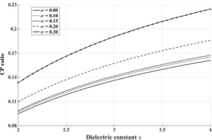
Figure 2.CP ratio as a function of dielectric constants for differ-entσ and incidence angle=30◦. The results for other incidence angles follow the similar trends.
By relating the CP ratio to the elements of the coherency matrix given for the X-SPM we obtain
CP ratio=
|6V|2
|6H|2 =
cc2|RS−RP|2|θl+ss2|RS−RP|2|θl
|RS+RP|2|θl
=
|RS−RP|2
|θl
|RS+RP|2
|θl
. (12)
Equation (12) shows that the CP ratio is controlled by ensem-ble averages of the difference and sum of the Bragg coeffi-cients with respect to the incidence angle. From del Monaco et al. (2009), the probability density function for cosθl is a normal distribution with mean cosθand standard deviation equal toσsinθ. After averaging over variations of the local incidence angleθl, the CP ratio is dependent on the dielectric constant of the surfaceε, the incidence angleθ, and the stan-dard deviation of the surface slopeσ. By using the model of del Monaco et al. (2009), the results of SAR measurements can be better explained than with the SPM.
We calculated the CP ratio as a function of the standard de-viation of surface slopeσ, assumingε=3.9+j0.15 which is suggested in Fung and Eom (1982) for first-year sea ice. The results show that the CP ratio increases with increasing stan-dard deviation of the surface slope at fixed incidence angles and with increasing incidence angle at fixedσ (Fig. 1). The relationship between the CP ratio and the dielectric constant is presented in Fig. 2. When the incidence angle is constant, the CP ratio reveals monotonically increasing values with in-creasing dielectric constant. A similar trend can also be found in the co-polarization ratio (Iodice et al., 2011). With respect to our simulated results shown in Figs. 1 and 2, it is impor-tant to note that the proposed parameter CP ratio is sensitive to the variation of the dielectric constant and almost insensi-tive to surface slope variations ifσ <0.15.
is only applicable under freezing conditions), and we do not consider metamorphosis of the basal snow layer due to brine wicking effects or due to melt–freeze cycles. We focus on undeformed Arctic young and first-year ice for which vol-ume scattering is low because of the relatively high ice salin-ity, which means that the ice surface is the dominant scatter-ing source. Then the backscatterscatter-ing coefficients depend on the small-scale surface roughness and the dielectric constant of the ice surface. Desalination of the ice occurs parallel to its growth due to brine drainage (Kovacs, 1996). The desali-nation process causes a decrease of the dielectric constant. Hence the basic idea of our method for retrieving ice ness is to relate changes of the dielectric constant to ice thick-ness growth. Because the CP ratio is sensitive to the varia-tion of the dielectric constant, it is well-suited for detecting changes of the ice thickness of smooth first-year level ice.
3 A simulation study
3.1 Forward scattering model
In this section, we describe the combined use of an ice growth model and an electromagnetic scattering model for level sea ice to study sensitivities of the CP ratio to different ice and radar properties. We applied the scattering model pro-posed by Nghiem et al. (1995) to simulate the sea ice volume scattering and absorption by brine inclusions. The surface contribution was calculated with the polarimetric two-scale model (Iodice et al., 2011, 2013) and incoherently added to the volume term.
The sea ice scattering model configuration is presented in Fig. 3. Note that we do not explicitly include a snow layer (see also Sect. 2.3). The effects of a dry snow layer are that (1) the dielectric contrast between ice and snow is lower than between ice and air, hence the reflectivity of the ice surface is lower; (2) the radar wavelength in the snow is shorter than in air, hence the ice surface appears rougher to the radar; (3) the incidence angle gets steeper (depend-ing on the dielectric constant of the snow), which (relatively) causes a stronger backscattering. Since we carry out simula-tions with different dielectric constants (by varying temper-ature and brine volume fraction), surface roughness parame-ters, and radar incidence angles, the results obtained without snow can be transferred to cases with dry snow layers.
In our model, the uppermost layer is air with permittiv-ityε0; the lowermost medium is seawater with complex per-mittivityε2, both enclosing the ice layer. The sea ice back-ground is assumed to be pure ice with complex permittiv-ity εi. The complex permittivity of brine inclusions is εb, and their fractional volume is fv. The relative permittivity of the sea iceεeffis a function of the volume fraction of brine inclusions (Arcone et al., 1986; Vant et al., 1978). The ice surface roughness is described by the correlation length l, rms heights, and the standard deviation of surface slopeσ.
The thickness and surface temperature of the sea ice layer areHandT0, respectively. Lastly, the magnetic permeability of free space isµ0. Thickness and permittivity of sea ice are subject to dynamic changes during the ice growth process. The small-scale surface roughness (on a centimeter scale) may also vary temporally and spatially. This, however, can hardly be measured in the field with sufficient spatial density over larger areas. Here we do not consider deformation pro-cesses causing surface roughness components on the order of meters. Furthermore, we assume that the scattering con-tribution of the ice–water interface can be neglected because of the relatively high salinity of Arctic young and first-year ice. Very thin ice, for which reflections of the radar waves between surface and bottom have to be considered, is ex-cluded from this study. In our simulations, we do not take snow cover into account. We restrict our analysis to tempera-tures well below freezing point, which means that a dry snow layer would change the incidence angle and the dielectric contrast at the ice surface. In the case of the ice growth sim-ulations described below, the snow has an insulating effect that changes the rate of ice thickness growth. Hence, various scenarios can be constructed, which is beyond the scope of this paper, which we regard as a first step towards developing a methodology for ice thickness retrieval using CP SAR.
For ice growth simulations we use a 1-D thermodynamic model developed by Maykut (1978, 1982) based on the en-ergy balance equations at the atmosphere–ocean boundary. The balance of the heat fluxes at the upper surface of the ice can be expressed as
(1−α)Fr−I0+FL−FE+Fs+FE+FC=0, (13) whereFris the incident short wave radiation,αFris the short wave radiation reflected by ice, andαis the albedo.I0is the amount of shortwave radiation absorbed in the interior of the ice layer,FLis the incoming long wave radiation,FEis the long wave radiation emitted by the ice,Fsis the sensible heat flux, andFEis the latent heat flux. The last termFCis the upward conductive heat flux that is the heat from the bottom interface conducted through the ice to the upper surface. We assume that the temperature at the ice–water interface is at
−1.8◦C. The equations and parameters used in this study are listed in Table 1.
Table 1.Equations and parameters used for the sea ice thermodynamic model.
Term Equations Parameters Comments
The incident short wave radiation
Fr=(1–0.0065C2)Qsoa m
(Ji et al., 2000; Yue et al., 2000)
am=0.99–0.17m am is the atmospheric
transmissivity;
C is the cloud coverage;
Qso is the solar irradiance for the
Dth day in a year;
Is is the solar radiation constant (unit: W/m2);
is the declination angle of the sun; Ha is the local solar hour angle; β and λ are the latitude and longitude; t is Coordinated Universal Time.
m=0.83
C in the range 0~1
Qso=Qs (sinβ sin + cosβ cos cosHa)
(Yue et al., 2000)
Qs=Is(1+0.033cos(2πD /365))
=23.44°cos[(172–
D)2π/365]
Ha=15(t-12)π/180+λ
The long wave radiation
4 0 iσT ε
FE
(Maykut, 1978)
σ=5.670×10⁻⁸ σ is the Stefan-Boltzman constant (unit: w/(m2K4));
T0 is the surface temperature of sea ice (unit: K);
Ta is the air temperature (unit: K);
εi is the emissivity of sea ice; εa is the emissivity of atmosphere;
e is the water vapor pressure at Ta (unit: HPa). εi=0.97 4 a 2 ) 1 ( a
L kC εσT
F
(Maykut, 1978)
k=0.0017
εa=0.55+e×0.0521/2
The sensible heat flux
Fs=ρaCpCsu(Ta-T0) (Cox and Weeks, 1988)
ρa=1.3 ρa is the air density (unit: kg/m
3 );
Cp is the specific heat at constant pressure (unit: J/(kg·K));
Cs is the sensible heat transfer coefficient;
u is the wind speed;
Cp=1006
Cs=0.003
The latent heat flux
Fe=ρaLCeu(qa-q0) (Cox and Weeks, 1988)
Ce=0.00175
L=2.5×10⁶–
2.274×10³(Ta–273.15)
L is the latent heat of vaporization (unit: J/kg); ) 1 ( ) ( ) ( ) ( ) ( 622 . 0 0 2 0 2 3 0 3 4 0 4 0 0 f e T fT d T fT c T fT b T fT a p q q a a a a a
(Cox and Weeks, 1988)
p0=1013
p0 is the surface atmospheric pressure (unit: mbar);
f is the relative humidity;
a, b, c, d, and e are constants;
a (unit: k4), b (unit: k3), c (unit: k2), d (unit: k)
a=2.7798202×10⁻⁶
b=-2.6913393×10⁻³
c=0.97920849; d=-158.63779 e=9653.1925; The albedo of sea ice
α=β0+β1 H +β2 H2+β3 H3
(Cox and Weeks, 1988)
β0=0.2386; β1=6.015×10⁻³ β2=-4.882×10⁻⁵; β3=1.267×10⁻⁷
H is the sea ice thickness (unit: cm).
The absorbed shortwave radiation
I0=i0(1–α)Fr
(Maykut, 1978; Cox and Weeks, 1988)
i0=17% i0 is the percent.
The upward conductive heat flux
FC = (k/H)(Tb–T0) (Cox and Weeks, 1988)
k = ki (1–fvb) + kb fvb
ki = 4.17×10⁴[5.35×10 -3–2.568×10⁻⁵(T
0– 273.15)]
kb = 4.17×10⁴[1.25×10 -3
+3.0×10⁻⁵(T0– 273.15)+1.4×10⁻⁷(T0– 273.15)2]
Tb=-1.8
k, ki, kb are the conductivity of ice layer, pure ice and pure brine, respectively (unit: W/m/K);
Tb is the freezing point at 35 salinity (unit: °C);
Table 2.Equations and parameters used for the sea ice properties.
Term Equations Parameters Comments
The ice thicknes s f C L ρ H F t
h ( )
Δ
Δ =
(Cox and Weeks, 1988)
∑
= = Time i Time t h H 0 Δ Δ ΔLf=4.187×10 3
(79.6 8–0.505Tb–
0.0273Si)+4.3115Si/ Tb+8×10⁻⁴Tb Si–
0.009(Tb)2
(Fukusako,1990)
is the sea ice growth
rate when ice thickness is
H (unit: m/s);
Ice thickness is the sum of ice growth rate.
ΔTime is the time lag (unit: hour). The sea ice density and brine volume fraction − = − = ) ( ) ( ) ( ) ( ) ( 2 1 2 1 1 i i i i i i i i i i i i T F S T F S f T F S T F T F ρ ρρ ρ ρ vb
(Cox and Weeks, 1983)
ρi=0.917-1.403×10
-4
Ti
ρ is sea ice density (unit: kg/m3);
fvbis the relative brine volume fraction
ρi is pure ice density (unit: kg/m3);
Ti is the temperature of sea ice (unit: °C);
Ta is the air temperature (unit: K);
Si is ice salinity.
The functional forms of F1 and F2 can be found from the work of Cox and Weeks (1983).
The ice salinity
> − = ≤ − = m) 4 . 0 ( 59 . 1 88 . 7 m) 4 . 0 ( 39 . 19 24 . 14 H H S H H S i i
(Cox and Weeks, 1983)
H is the ice thickness (unit:
m). The permitti vity of sea ice at C-band vb eff f
ε′ =3.05+0.0072
vb eff f
ε′′ =0.02+0.0033 (Arcone et al., 1986; Vant et al., 1978)
fvbis the relative brine volume fraction.
Figure 3.Structure and geometric model of the configuration of sea ice.
surface roughness parameterss,l, andσ are set to different values considering the validity range of the X-SPM model (Ulaby et al., 1982; del Monaco et al., 2009; Iodice et al., 2011).
3.2 Simulation results
Figure 4.The simulated sea ice growth process. Blue: sea ice thick-ness; red: sea ice surface temperature; green: the volume fraction of brine inclusions.
l=1.26 cm (kl=0.035,ks=1.4 for the radar frequency of 5.4 GHz, k – wavenumber) for dark nilas, (2) s=0.12 cm and l=1.45 cm (kl=0.14, ks=1.6) for light nilas, and (3) s=0.11 cm andl=0.54 cm (kl=0.12 andks=0.6) for smooth first-year ice. We note that we will use these rough-ness values for first-year ice in general, considering the large variability of small-scale ice surface roughness. The values are in the validity range of the original Bragg scattering the-ory and should hence be fully covered by the X-SPM model presented in Iodice et al. (2011). The standard deviation of the large-scale slopeσranges according to the validity range of the X-SPM model (Iodice et al., 2011).
At this point we note that a systematic relationship be-tween small-scale surface roughness and ice thickness has never been reported. Weathering effects, melt events, and snow metamorphism influence the millimeter-to-centimeter ice surface roughness to a highly variable extent, indepen-dent of ice thickness. As we will show below, the influence of the small-scale roughness on the CP ratio is moderate to low; hence the issue of varying small-scale surface roughness is not very critical.
Figure 4 illustrates the simulated sea ice thickness as a function of time and ice temperature, and the volume frac-tion of brine inclusions as funcfrac-tions of ice thickness. Figure 4 clearly shows that the volume fraction of brine inclusions re-duces due to desalination processes as the ice thickness in-creases.
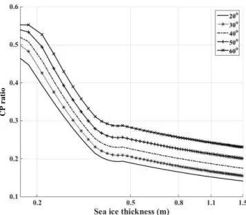
To investigate the dependence of the CP ratio on the radar incidence angle and ice thickness, the complex scattering co-efficients (SHH, SVV, and SHV) were computed for the C-band (5.4 GHz) at incidence angles of 20–60◦. Then the CP ratio was calculated from Eq. (12). The relationship between the CP ratio and sea ice thickness in case 3 (first-year ice
CP ratio
Figure 5.The relationship between the CP ratio and ice thickness at different incidence angles for C-band radar (xaxis on a log scale). The incidence angle varies from 20 to 60◦. The small-scale rough-ness parameters are set tos=0.11 cm andl=0.54 cm (case 3), the standard deviation of the surface slopeσ=0.1.
roughness conditions given above) andσ=0.1 is shown in Fig. 5. It reveals that the CP ratio exhibits a monotonically decreasing trend with growing ice thickness at constant in-cidence angles. It should be noted that the sensitivity of the CP ratio to vertical ice growth is much higher at smaller ice thickness values up to approximately 0.4 m. This can be ex-plained by fact that the ice salinity is calculated according to the relationship proposed by Cox and Weeks (1983). Their parameterization of salinity as a function of ice thickness re-veals a discontinuity at a thickness of 0.4 m.
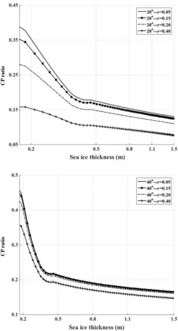
Figure 6.Sensitivity of the CP ratio to the standard deviation of the surface slopeσ (xaxis in log scale). The standard deviation of the surface slopeσ varies from 0.05 to 0.4, while the small-scale roughness is fixed ats=0.12 cm andl=1.45 cm (case 2). The top panel is for the 20◦incidence angle and the bottom panel is for the 40◦incidence angle.
(<0.4 m) than for thicker sea ice. At larger incidence angles, the reduction of the radar wavelength in a snow layer on top of the ice is not a critical issue, since the effect of the small-scale roughness on the CP ratio is low in this case. However, the snow layer also changes the incidence angle of the radar beam on the ice surface, which can have a considerable im-pact on the thickness retrieval, in particular at thickness val-ues larger than 0.3 to 0.4 m where the slope of the curves theoretically decreases to a low value (Fig. 7). In practice, this limitation is less critical as we show below. On first-year
CP ratio
Figure 7.Sensitivity of the CP ratio to the small-scale roughness (xaxis in log scale). The standard deviation of the surface slopeσ is fixed at 0.1. Black, blue, red, green and cyan colors are for 20, 30, 40, 50, and 60◦incidence angles, respectively. In the legend, C1, C2, and C3 denote the three cases of small-scale surface rough-ness respectively (C1:s=0.031 cm,l=1.26 cm; C2:s=0.12 cm, l=1.45 cm; C3:s=0.11 cm,l=0.54 cm).
sea ice, the bottom part of the snow layer can be saline due to brine wicking, possibly creating a dielectric interface within the snow, or resulting in brine volumes large enough to influ-ence the radar backscatter (Barber and Nghiem, 1999; Galley et al., 2009). This may also affect the accuracy of the thick-ness retrieval using the CP ratio. Finally, we note that the model simulations include interactions between the ice sur-face and the ice–water intersur-face, which result in oscillations of the CP ratio for an ice thickness<0.16 m. In the field mea-surements discussed below, this effect was not observed. We assume that the actual ice thickness is rarely exactly constant over larger areas.
4 Datasets and experimental results 4.1 Field study
Figure 8.Location of the study site in the Labrador Sea, with Pauli RGB (HH+VV for blue, HH−VV for red, and HV for green) de-compositions of the RADARSAT-2 images©MDA. The specifica-tions of the SAR data used are given in Table 3.
the ice thickness values derived from such soundings agree well within±0.1 m over flat homogeneous ice (Haas et al., 2006; Prinsenberg et al., 2012b). The accuracy decreases over ridges and deformed ice, where the maximum thick-ness can be underestimated by as much as 50 % (Haas et al., 2006; Prinsenberg et al., 2012b). Snow thickness pro-files were collected concurrently with a ground-penetrating radar (GPR) and the laser altimeter measurements. The ground-penetrating radar, which was operated at a frequency of 1 GHz, receives returns from the ice–snow and air–snow interfaces, though the return from air–snow surface is very weak. The laser altimetry is superior for defining the air– snow interface. Therefore, the combination of the GPR and laser altimetry allows the snow depth on sea ice to be re-trieved. For a 1 GHz GPR system, the minimum detectable snow layer thickness is 0.12 m and the measurement error is 0.08 m in light dry snow (Lalumiere, 2006). By subtracting the GPR snow thickness measurements from the EMS snow
Table 3.Specifications of the qual-pol RADARSAT-2 SAR data.
Scene Date/time Resolution (m)∗ Incidence Beam
ID (UTC) Rng×Az angle mode
(deg.)
No. 1 19 Mar 2011, 10:25 5.2×7.7 29.0 FQ9 No. 2 19 Mar 2011, 21:51 5.2×7.7 42.0 FQ23 No. 3 19 Mar 2011, 21:51 5.2×7.7 42.0 FQ23 No. 4 20 Mar 2011, 09:56 5.2×7.7 49.0 FQ31
∗Resolution is nominal. Ground range resolution varies with incidence angle.
plus ice thickness measurements, sea ice thickness can be es-timated.
4.2 Data sets and data processing
All data are available on the website of DFO in-cluding pictures, notes, and reports of the survey (http://www.bio.gc.ca/science/research-recherche/ocean/ ice-glace/data-donnees-eng.php).
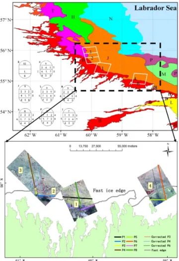
During the field survey, four C-band RADARSAT-2 quad-polarization images were acquired nearly coincident with the DFO airborne survey flight lines (Fig. 8). The RADARSAT-2 data were provided by the MacDonald, Dettwiler and As-sociates Ltd (MDA). Important SAR parameters are listed in Table 3. For our processing we used the RADARSAT-2 single-look slant range complex format as starting point. A speckle reduction filter (13×13 Lee filter) and radiometric calibration procedures were applied for the calculation of the scattering matrix. With the quad-polarization data, the CTLR compact polarimetry mode can be generated via Eq. (3). Sub-sequently the CP ratio was extracted by Eq. (11). Lastly, the geometric registration of the simulated CP SAR images (i.e., their representation in geographical coordinates) was performed based on longitude and latitude data provided in SAR metadata.
Table 4.Specifications of helicopter-borne EMS ice thickness data sets.
EM SAR scene ID Date/time Time
ID coincident (UTC) difference
with EMS
P-1 no. 1 19 Mar 2011, 17:00–17:20 ∼7 h P-2 no. 2 19 Mar 2011, 17:25–17:30 ∼4 h P-3 no. 2 19 Mar 2011, 18:30–18:45 ∼3.3 h P-4 no. 3 19 Mar 2011, 18:40–18:50 ∼3 h P-5 no. 4 20 Mar 2011, 11:55–12:05 ∼2 h P-6 no. 4 20 Mar 2011, 12:10–12:25 ∼2.5 h P-7 no. 1 20 Mar 2011, 14:25–14:30 ∼28 h P-8 no. 1 20 Mar 2011, 14:40–14:50 ∼28 h
data archive from Makkovik station (http://climate.weather. gc.ca/), the air temperature was around−9 to−17◦C on 15– 16 March 2011, and snowfall was registered during 2 days in the period 17–19 March with average air temperature around
−15◦C. Therefore, a large fraction of the sea ice was cov-ered with snow, which can be clearly seen in aerial photos (not shown). On 19–20 March 2011, the average air temper-ature was around−8 to−12◦C and the wind speed around 11–15 m s−1(Prinsenberg et al., 2012a). Hence the snow can be regarded as dry. We also note that thermodynamically driven effects on the bottom snow layer such as brine wick-ing take place at temperatures higher than−7◦C (Barber and Nghiem, 1999) which means that we can ignore them here for the freshly fallen snow. However, we do not have any in-formation about elder snow layers changed by metamorpho-sis processes, which may have an influence on the effective backscattering signature; nor can we exclude the fact that sea ice flooding took place in some smaller areas. Figure 9 shows the ice thickness and snow depth profiles of the land-fast and drift ice, indicating that the ice freeboard was mostly above the water level. The histograms shown in Fig. 9 confirm that the land-fast mean ice thickness is smaller than the one of the drifting pack ice. The percentages of areas with snow thickness above 0.2 m for land-fast and drift ice are 26.4 and 18.2 % respectively. The flight profiles also show that there are deformed ice or ridges (ice thickness exceeded 2.0 m) in the survey field.
A direct comparison between SAR imagery and flight pro-files’ data may cause errors due to the time differences of the data acquisitions (the time difference between SAR and flight data is shown in Table 4). In addition, spatial differences may be caused by the different sampling and spatial resolutions of the measurement instruments. The sampling rate for the EMS and the laser is 10 Hz, which, given a typical helicopter survey speed of 80 mph, corresponds to a spatial sampling interval of about 3–4 m. While the footprint size of the laser is very small (several centimeters), the footprint of the EMS is around 20 m at a typical operation height of 5–6 m. For this experiment, the GPR was configured to a scan rate of
approx-Figure 9.Histogram of ice and snow thickness in the Labrador Sea.
imately 30 scans per second. When flying at 60–80 knots, the ground sample spacing is approximately one sample per 1.0–1.5 m. Moreover, according to the DFO survey report, the floating ice drifted 1.4–1.8 knots towards the southeast, as measured by ice beacons (Prinsenberg et al., 2012a). In order to mitigate the errors caused by time and spatial res-olution differences, we used the following processing chain for linking SAR and airborne data.
1. The correction of the time difference was only imple-mented for the drifting ice region. The boundary be-tween fast ice and drifting pack ice was taken from ice charts of the Canadian Ice Service (Fig. 8). Of the eight EMS profiles, P1, P2, P5, and P7 are in or near the land-fast ice region, whereas P3, P4, P6, and P8 are from the drift ice zone. With an ice drift speed of 1.5 knots, and drift direction southeast taken from the DFO survey re-port and considering the respective time differences, the profiles P3, P4, P6, and P8 are shifted to their approx-imate positions at the acquisition time of the SAR im-ages. The shifted profiles are presented in Fig. 8 (dotted line). It should be noted that 28 h passed between the acquisition times of the P8 and SAR data, and the cor-rected location of P8 is beyond the coverage of the SAR image. Hence P8 was discarded from further analysis. 2. The EMS (ice plus snow) thickness values below 0.1 cm
were removed to consider the measurement accuracy of the EMS. Regions for which only EMS data but no GPR data are available were also removed.
3. Regions with GPR snow thickness values higher than 0.20 m were removed, because snow layers thinner than 0.20 m are nearly transparent to C-band radar waves, and the backscatter from the snow surface and volume can be neglected (Hall et al., 2006).
4. By combining the field survey data (ice charts and aerial photos), a visual interpretation of RADARSAT-2 SAR was made, and regions of open water, land, and de-formed ice were masked in the SAR images. Land was identified using the coastal line; open water areas were interpreted via backscattering and texture. Deformed ice was brighter than level ice in single-polarization SAR images, and revealed a higher entropy, which was ex-tracted using H /A/α decomposition (Scheuchl et al., 2002). We emphasize that in step 2, most open water areas are already excluded from further analysis. 5. For ice zones of 50 m in length, averages of different
parameters were evaluated. Firstly, we used theH /A/α unsupervised Wishart classifier to segment the SAR im-ages, and each patch was regarded a homogeneous ice area with respect to its radar signature. Then the snow thickness, snow plus ice thickness profiles were cut into flight track segments 50 m long. The CP ratio values
were evaluated from the co-located, drift-corrected, seg-mented SAR images, provided that the 50 m segment contained a homogeneous piece of ice. The segment length of 50 m was chosen according to the spatial res-olution of the SAR image. Range and azimuth spacing of a RADARSAT-2 fine quad-polarization product are 4.7 m×4.9 m respectively. Since we applied a 13×13 window for speckle reduction (see above), the effective spatial resolution is about 50 m. For the averages along transects, 13 SAR pixels, 15 EMS samples, and 45 GPR samples were used.
6. The sea ice thickness was extracted from the averaged GPR snow depth and EMS snow plus ice thickness val-ues.
7. Finally we calculated the CP ratio from Eq. (11) using the averaged complex backscattering coefficients. This processing chain ensures that only level ice is consid-ered for which the EMS system delivers reliable thickness data with an acceptable accuracy. The total length of the pro-file segments that we used in this study amounts to about 16 km (320 samples). Compared with the original data, al-most 60 % of the data were discarded in this processing chain (step 1: 17 %, step 2: 10 %, step 3: 23 %, step 4: 10 %). 4.3 Ice thickness retrieval
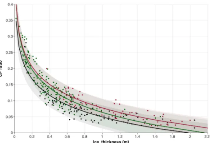
To investigate the possibility of using the proposed polari-metric parameter CP ratio to estimate sea ice thickness from SAR images, we plotted ice thickness values obtained during the field campaign against the corresponding values of the CP ratio derived from the RADARSAT-2 images in Fig. 10 (using all 320 samples). It can be seen that at C-band, the CP ratio shows a negative trend relative to the ice thick-ness as the simulated results given in Sect. 3.2 predicted. Figure 10 reveals that the highest sensitivity occurs between 0 and 0.5 m and saturates with thickness values exceeding 1.5 m. As shown in Figs. 5 to 7, the sensitivity should be smaller for ice thickness exceeding 0.4 m. However, the slope change of the curves at 0.4 m is not as abrupt as in the theo-retical curves predicted in Sect. 3.2. This can be presumably explained by the fact that we average over segments with dif-ferent values of ice roughness parameterss,l, andσ. We also need to consider that the salinity–thickness parameterization proposed by Cox and Weeks (1983) includes a discontinu-ity in the slope of the salindiscontinu-ity curve at a thickness of 0.4 m, which may not exist in reality.
Figure 10.Regressions relating ice thickness to CP ratio at different incidence angles. The solid lines represent the fits, dashed lines the 90 % confidence intervals. The black, green and red colors are used for the incidence angles of 29, 42 and 49◦, respectively.
For Fig. 10, the empirical equations and correlation coeffi-cients (CC) are
( CP ratio=0.04935−0.07329 ln(H ) for 29◦incident angle(CC=0.90)
CP ratio=0.06345−0.08251 ln(H ) for 42◦incident angle(CC=0.93)
CP ratio=0.07744−0.07952 ln(H ) for 49◦incident angle(CC=0.89), (14)
where all data points (320 samples) are used to derive the em-pirical regressions in the thickness range from 0.1 to 1.8 m. The reason to include larger ice thickness values is that they can be measured with a larger accuracy, hence leading to a more robust relationship at least for the moderate thickness values between 0.4 and 0.8 m. However, to our knowledge the distribution of the CP ratio due to speckle has not been derived yet which makes it difficult to judge its variation. The smallest values of the CP ratio observed are about 0.03, which may indicate the noise level of the CP ratio. The mea-sured values of the CP ratio for ice thickness values>0.2 m shown in Fig. 10 are lower than the theoretical computations. This can presumably be explained by the fact that underly-ing theoretical models are an oversimplification of the ac-tual situation. We note that due to the limitation of sample points, the fit for 49◦incident angle is mainly determined by ice thickness values>0.5 m.
We found that the level of the CP ratio increases as the in-cidence angle increases at a given value of the sea ice thick-ness. This observation compares well with the forward sim-ulation studies as shown in Fig. 5. These high correlations enable us to derive reliable thickness information for smooth level ice from radar images, assuming winter conditions (dry snow, no brine wicking). The ice thickness can be estimated using an exponential function, which can be described as fol-lows:
H=exp a
−(CP ratio) b
, (15)
whereaandbare the coefficients of the exponential fit.
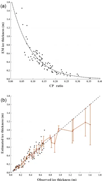
At the next stage, we focused on the RADARSAT-2 im-ages no. 2 and no. 3 (which have the same incidence angle of 42◦) to validate our method. Out of a total of 320 sam-ples, 159 samples belong to images no. 2 and no. 3. Accord-ing to the principle of independent sample tests, we divided these 159 samples into two data sets in an arbitrary way. The first set includes 79 samples that are used to fit the model for estimating ice thickness, and the second one comprises 80 samples that serve to retrieve ice thickness and compare the results with the data from the field campaign. The coef-ficientsa andbof the empirical fit generated from the first data set are 0.068 and 0.077 respectively. Note that these co-efficients are different from those derived in Eq. (14) from the same two SAR images because now fewer points could be used to derive the fit. The fitted curve and validation re-sults are presented in Fig. 11a and b, respectively. The cor-relation coefficient for the fit shown in Fig. 11a is 0.93 for the thickness range from 0.1 to 1.8 m and 0.94 for the thick-ness range from 0.1 to 0.8. The rms error and the relative error between the observed and the estimated ice thickness, shown in Fig. 11b, are 12 cm and 20 % in the thickness range from 0.1 to 1.8 m, and 8 cm and 17 % for 0.1 to 0.8 m. The relative rms error implies, e.g., that the absolute rms error is 0.2 m at an ice thickness of 1.0 m (for the range 0.1 to 1.8 m). Figure 11b also demonstrates that the error of the re-trieved ice thickness is very large at values>0.8 m which is to be expected from the theoretical curves, considering the significantly decreased sensitivity of the CP ratio to larger ice thickness.
5 Discussion and conclusion
This paper provides a first analysis of sea ice thickness re-trieval using compact polarimetric SAR. We developed a new parameter that we call the CP ratio to estimate the thickness of undeformed first-year level ice from C-band radar images, under dry snow conditions (snow depth<20 cm). Numeri-cal model simulations showed that this parameter is sensitive to changes of the dielectric constant that are linked to the growth of sea ice. We developed empirical relationships for the retrieval of level ice thickness from CP ratios. For the validation of our results we also employed RADARSAT-2 images for which thickness values were available. The opti-mal regression between the CP ratio and ice thickness was achieved with an exponential fit. The rms error was 12 cm, and the relative error amounted to 20 % for a thickness range between 0.1 and 1.8 m, and 8 cm and 17 % for the range be-tween 0.1 and 0.8 m. This indicates that the proposed param-eter is very useful for the retrieval of first-year level ice thick-ness between 0.1 and 0.8 m.
Figure 11. (a)Relationship between the CP ratio and the observed EM sea thickness.(b)Comparison between the observed and esti-mated ice thicknesses, and the error bars show the standard devia-tion with respect to the observadevia-tion data for every 0.05 m segment of ice thickness.
ice, which reveals a larger variation of large-scale roughness with respect to the sensor resolution, needs to be further dis-cussed and studied.
Although our tests are performed on a limited sample of images, our findings demonstrate that the C-band compact polarimetric SAR has a potential for sea ice thickness re-trievals over level first-year ice covered by a thin dry snow-pack. The issue of environmental factors affecting the re-trieval accuracy, e.g., brine wicking in the snow, or snow lay-ers with different dielectric properties, has to be investigated further in more detail. The several planned Earth-observing satellite missions supporting compact polarimetry (e.g., the RCM operated at C-band) will provide the wide swath
cover-age necessary for operational sea ice monitoring. Hence our approach potentially provides a new operational tool for sea ice thickness measurements with a large areal coverage. In this case, the resulting thickness products are also of interest for the development, improvement, and validation of fore-cast models for the prediction of ice conditions, or of interest for seasonal and climate simulations that consider Arctic and Antarctic ice conditions.
Acknowledgements. This study was supported by the National
Nature Science Foundation of China under grant 41306193, and the R & D Special Foundation for Public Welfare Indus-try (201305025). This work was carried out as part of the Dragon-3 Programme (10501) by the Ministry of Science and Technology of the P. R. China and the European Space Agency. The authors would like to thank the Canadian Space Agency (CSA) and MDA for providing the RADARSAT-2 data, and we are very thankful to the Department of Fisheries and Oceans Canada for their support in providing valuable snow and sea ice field data. We gratefully acknowledge the detailed comments of Stefan Kern and two anonymous reviewers which helped to considerably improve the readability of the article.
Edited by: C. Duguay
References
Arcone, A., Gow, A. G., and McGrew, S.: Structure and dielectric properties at 4.8 and 9.5 GHz of saline ice, J. Geophys. Res., 91, 14281–14303, 1986.
Barber, D. G. and Nghiem, S. V.: The role of snow on the thermal dependence of microwave backscatter over sea ice, J. Geophys. Res., 104, 25789–25803, 1999.
Behrendt, A., Dierking, W., Fahrbach, E., and Witte, H.: Sea ice draft in the Weddell Sea, measured by upward looking sonars, Earth Syst. Sci. Data, 5, 209–226, doi:10.5194/essd-5-209-2013, 2013.
Charbonneau, F. J., Brisco, B., Raney, R. K., McNairn, H., Liu, C., Vachon, P., Vachon, W., Shang, J., DeAbreu, R., Champagne, Merzouki, A., and Geldsetzer, T.: Compact polarimetry overview and applications assessment, Can. J. Remote Sens., 36, 298–315, 2010.
Cox, G. and Weeks, W.: Equations for determining the gas and brine volumes in sea-ice samples, J. Glaciol., 29, 306–316, 1983. Cox, G. and Weeks, W.: Numerical simulations of the profile
prop-erties of undeformed first-year sea ice during the growth season, J. Geophys. Res., 93, 12449–12460, 1988.
Dabboor, M. and Geldsetzer, T.: Towards sea ice classification us-ing simulated RADARSAT Constellation Mission compact po-larimetric SAR imagery, Remote Sens. Environ., 140, 189–195, 2014.
Dierking, W.: Laser profiling of the ice surface topography during the Winter Weddell Gyre Study 1992, J. Geophys. Res., 100, 4807–4820, 1995.
Dierking, W.: Sea ice monitoring by synthetic aperture radar, Oceanography, 26, 100–111, doi:10.5670/oceanog.2013.33, 2013.
Fukusako, S.: Thermophysical properties of ice, snow, and sea ice, Int. J. Thermophys., 11, 353–372, 1990.
Fung, A. K.: Microwave Scattering and Emission Models and Their Applications, Artech House, Boston, London, 1994.
Fung, A. K. and Eom, H. J.: Application of a combined rough sur-face and volume scattering theory to sea ice and snow backscat-ter, IEEE T. Geosci. Remote, GE-20, 528–536, 1982.
Galley, R. J., Trachtenberg, M., Langlois, A., Barber, D. G., and Shafai, L.: Observations of geophysical and dielectric proper-ties and ground penetrating radar signatures for discrimination of snow, sea ice and freshwater ice thickness, Cold Reg. Sci. Tech-nol., 57, 29–38. 2009.
Geldsetzer, T., Arkett, M., Zagon, T., Charbonneau, F., Yackel, J. J., and Scharien, R.: All season compact-polarimetry SAR observations of sea ice, Can. J. Remote Sens., 41, 485–504, doi:10.1080/07038992.2015.1120661, 2015.
Goebell, S.: Comparison of coincident snow-freeboard and sea ice thickness profiles derived from helicopter-borne laser altimetry and electromagnetic induction sounding, J. Geophys. Res., 116, C08018, doi:10.1029/2009JC006055, 2011.
Haapala, J., Lensu, M., Dumont, M., Renner, A. H. H., Granskog, M. A., and Gerland, S.: Small-scale horizontal variability of snow, sea-ice thickness and freeboard in the first-year ice region north of Svalbard, Ann. Glaciol., 54, 261–266, doi:10.3189/2013AoG62A157, 2013.
Haas, C., Gerland, S., Eicken, H., and Miller, H.: Comparison of sea-ice thickness measurements under summer and winter con-ditions in the Arctic using a small electromagnetic induction de-vice, Geophysics, 62, 749–757, 1997.
Haas, C., Hendricks, S., and Doble, M.: Comparison of the sea ice thickness distribution in the Lincoln Sea and adjacent Arc-tic Ocean in 2004 and 2005, Ann. Glaciol., 44, 247–252, 2006. Hajnsek, I., Pottier, E., and Cloude, S. R.: Inversion of surface
pa-rameters from polarimetric SAR, IEEE T. Geosci. Remote, 41, 727–744, 2003.
Hall, D. K., Kelly, R. E., Foster, J. L., and Chang, A. T.: Estimation of Snow Extent and Snow Properties, Encyclopedia of Hydrolog-ical Sciences, 5–55, 2006.
Hendricks, S., Gerland, S., Smedsrud, L. H., Hass, C., Pfaffhuber, A., and Nilsen, F.: Sea-ice thickness variability in Storfjorden, Svalbard, Ann. Glaciol., 52, 61–68, 2011.
Huntemann, M., Heygster, G., Kaleschke, L., Krumpen, T., Mäky-nen, M., and Drusch, M.: Empirical sea ice thickness retrieval during the freeze-up period from SMOS high incident angle ob-servations, The Cryosphere, 8, 439–451, doi:10.5194/tc-8-439-2014, 2014.
Iodice, A., Natale, A., and Riccio, D.: Retrieval of soil surface pa-rameters via a polarimetric two-scale model, IEEE T. Geosci. Re-mote, 49, 2531–2547, 2011.
Iodice, A., Natale, A., and Riccio, D.: Polarimetric two-scale model for soil moisture retrieval via dual-Pol HH-VV SAR data, IEEE J. Sel. Top. Appl., 6, 1163–1171, 2013.
Ji, S. Y., Yue, Q. J., and Zhang, X.: Thermodynamic analysis during sea ice growth in the Liaodong Bay, Mar. Environ. Sci., 19, 35– 39, 2000.
Kim, J. W., Kim, D. J., and Hwang, B. J.: Characterization of Arctic sea ice thickness using high-resolution spaceborne polarimetric SAR data, IEEE T. Geosci. Remote, 50, 13–22, 2012.
Kovacs, A.: Sea Ice, Part I.: Bulk Salinity versus Ice Floe Thick-ness, USA Cold Regions Research and Engineering Laboratory, CRREL Rep. 97, United States Army, Corps of Engineers, Wash-ington, D.C., 1–16, 1996.
Kovacs, A., Valleau, N. C., and Holladay, J. S.: Airborne electro-magnetic sounding of sea ice thickness and sub-ice bathymetry, Cold Reg. Sci. Technol., 14, 289–311, 1987.
Kwok, R.: Satellite remote sensing of sea ice thickness and kine-matics: a review, J. Glaciol., 56, 1129–1140, 2010.
Kwok, R. and Cunningham, G. F.: ICESat over Arctic sea ice: Es-timation of snow depth and ice thickness, J. Geophys. Res., 113, C08010, doi:10.1029/2008JC004753, 2008.
Kwok, R., Nghiem, S. V., Yueh, S. H., and Huynh, D. D.: Retrieval of thin ice thickness from multifrequency polarimetric SAR data, Remote Sens. Environ., 51, 361–374, 1995.
Kwok, R., Cunningham, G. F., Wensnahan, M., Rigor, I., Zwally, H. J., and Yi, D.: Thinning and volume loss of the Arctic Ocean sea ice cover: 2003–2008, J. Geophys. Res., 114, C07005, doi:10.1029/2009JC005312, 2009.
Lalumiere, L.: Ground penetrating radar of helicopter snow and ice surveys, Can. Tech. Rep. Hydrogr. Ocean Sci., 248, 1–50, http://publications.gc.ca/collections/collection_2015/ mpo-dfo/Fs97-18-248-eng.pdf (last access: 7 July 2016), 2006. Laxon, S. W., Giles, K. A., Ridout, A. L., Wingham, D. J., Willatt,
R., Cullen, R., Kwok, R., Schweiger, A., Zhang J., Haas, C., Hen-dricks, S., Krishfield, R., Kurtz, N., Farrell, S. and Davidson, M.: CryoSat-2 estimates of Arctic sea ice thickness and volume, Geo-phys. Res. Lett., 40, 732–737, doi:10.1002/grl.50193, 2013. Maykut, G. A.: Energy exchange over young sea ice in the central
Arctic, J. Geophys. Res., 83, 3646–3658, 1978.
Maykut, G. A.: Large-scale heat exchange and ice production in the central Arctic, J. Geophys. Res., 87, 7991–7984, 1982.
Nakamura, K., Wakabayashi, H., Naoki, K., Nishio, F., Moriyama, T., and Uratsuka, S.: Observation of sea-ice thickness in the sea of Okhotsk by using dual-frequency and fully polarimetric air-borne SAR (Pi-SAR) data, IEEE T. Geosci. Remote, 43, 2460– 2469, 2009a.
Nakamura, K., Wakabayashi, H., Uto, S., Ushio, S., and Nishio, F.: Observation of sea-ice thickness using ENVISAT data from Lützow-Holm Bay, East Antarctica, IEEE Geosci. Remote Sens. Lett., 6, 277–281, 2009b
Nghiem, S. V., Kwok, R., Yueh, S. H., and Drinkwater, M. R.: Po-larimetric signatures of sea ice, theoretical model, J. Geophys. Res., 100, 13665–13679, 1995.
Nord, M. E., Ainsworth, T. L., Lee, J. S., and Stacy, N. J. S.: Com-parison of compact polarimetric synthetic aperture radar modes, IEEE T. Geosci. Remote, 47, 174–188, 2009.
Onstott, R.: SAR and scatterometer signatures of sea ice, in: Mi-crowave Remote Sensing of Sea Ice, Geophysical Mono. 68, edited by: Carsey, F., Amer. Geophys. Union, Washington, D.C., 73–104, 1992.
Can. Tech. Rep. Hydrogr. Ocean Sci., 275, 1–44, http://www. ocean-sci.net/275/1/2012/ (last access: 7 July 2016), 2012a. Prinsenberg, S. J., Hollady, S., and Lee, J.: Measuring ice thickness
with EISflow, a fixed-mounted helicopter electromagnetic-laser system, Proc. 12th International Off-shore and Polar Engineering Conference, Kitakyushu, Japan, 737–740, 2012b.
Raney, R.: Hybrid polarity SAR architecture, IEEE T. Geosci. Re-mote, 45, 3397–3404, 2007.
Rossiter, J. R. and Holladay, J. S.: Ice-thickness measurement, in: Remote Sensing of Sea Ice and Icebergs, edited by: Haykin, S., Lewis, O. E., Raney, R. K., and Rossite, J. R., John Wiley, Hobo-ken, NJ, 141–176, 1994.
Rothrock, D. A., Yu, Y., and Maykut, G. A.: Thinning of the Arctic sea-ice cover, Geophys. Res. Lett., 26, 3469–3472, doi:10.1029/1999GL010863, 1999.
Scheuchl, B., Hajnsek, I., and Cumming, I.: Sea ice classification using multi-frequency polarimetric SAR data, in: Geosci. Re-mote Sens. Symposium, IGARSS’02, Toronto, Canada, 1914– 1916, 2002.
Scheuchl, B., Flett, D., Caves, R., and Cumming, I.: Potential of RADARSAT-2 data for operational sea ice monitoring, Can. J. Remote Sens., 30, 448–461, 2004.
Soulis, E. D., Lennox, W. C., and Sykes, J. F.: Estimation of the thickness of undeformed first year ice using radar backscatter, in: Geosci. Remote Sens. Symposium, IGARSS’89, Vancouver, Canada, 2366–2369, 1989.
Souyris, J. C., Imbo, P., Fjortoft, R., Mingot, S., and Lee, J. S.: Com-pact polarimetry based on symmetry properties of geophysical media: Theπ/4 mode, IEEE T. Geosci. Remote, 43, 634–646, 2005.
Tian-Kunze, X., Kaleschke, L., Maaß, N., Mäkynen, M., Serra, N., Drusch, M., and Krumpen, T.: SMOS-derived thin sea ice thick-ness: algorithm baseline, product specifications and initial ver-ification, The Cryosphere, 8, 997–1018, doi:10.5194/tc-8-997-2014, 2014.
Toyota, T., Nakamura, K., Uto, S., Ohshima, K. I., and Ebuchi, N.: Retrieval of sea ice thickness distribution in the seasonal ice zone from airborne L-band SAR, Int. J. Remote Sens., 30, 3171–3189, 2009.
Ulaby, F. T., Moore, R. K., and Fung, A. K.: Microwave Remote Sensing: Active and Passive, vol. II, Addison-Wesley, Reading, MA, 1982.
Vancoppenolle, M., Fichefet, T., and Bitz, C. M.: On the sensitiv-ity of undeformed Arctic sea ice to its vertical salinsensitiv-ity profile, Geophys. Res. Lett., 32, L16502, doi:10.1029/2005GL023427, 2005.
Vant, M. R., Ramseier, R. O., and Makios, V.: The complex dielec-tric constant of sea ice at frequencies in the range 0.1 to 40 GHz, J. Appl. Phys., 49, 1264–1280, 1978.
Wadhams, P.: A comparison of sonar and laser profiles along cor-responding tracks in the Arctic Ocean, in: Sea Ice Processes and Models, edited by: Pritchard, R. S., Univ. of Washington Press, Seattle, Washington, 283–299, 1980.
Wadhams, P., Tucker III, W. B., Krabill, W. B., Swift, R. N., Comiso, J. C., and Davis, N. R.: Relationship between sea ice freeboard and draft in the Arctic Basin, and implications for ice thickness monitoring, J. Geophys. Res., 97, 20325–20334, doi:10.1029/92JC02014, 1992.
Wakabayashi, H., Matsuoka, T., and Nakamura, K.: Polarimetric characteristics of sea ice in the Sea of Okhotsk observed by air-borne L-band SAR, IEEE T. Geosci. Remote, 42, 2412–2425, 2004.