True-and-error models violate independence and yet they are
testable
Michael H. Birnbaum
∗Abstract
Birnbaum (2011) criticized tests of transitivity that are based entirely on binary choice proportions. When assump-tions of independence and stationarity (iid) of choice responses are violated, choice proporassump-tions could lead to wrong conclusions. Birnbaum (2012a) proposed two statistics (correlation and variance of preference reversals) to test iid, using random permutations to simulatep-values. Cha, Choi, Guo, Regenwetter, and Zwilling (2013) defended methods based on marginal proportions but conceded that such methods wrongly diagnose hypothetical examples of Birnbaum (2012a). However, they also claimed that “true and error” models also satisfy independence and also fail in such cases unless they become untestable. This article presents correct true-and-error models; it shows how these models violate iid, how they might correctly identify cases that would be misdiagnosed by marginal proportions, and how they can be tested and rejected. This note also refutes other arguments of Cha et al. (2013), including contentions that other tests failed to violate iid “with flying colors”, that violations of iid “do not replicate”, that type I errors are not appropriately estimated by the permutation method, and that independence assumptions are not critical to interpretation of marginal choice proportions.
Keywords:
1
Introduction
Although there is much to admire in the approach of Regenwetter, Dana, and Davis-Stober (2011) for test-ing transitivity in choice experiments, Birnbaum (2011) criticized its focus on marginal choice proportions rather than response patterns. Birnbaum pointed out that when choice responses are not independent and identically dis-tributed (iid), any method based strictly on marginal choice proportions could easily reach wrong substantive conclusions.
The main problem is that data generated from mixtures that include intransitive preference patterns can appear to satisfy transitivity by such methods. Birnbaum (2011) therefore suggested that one should analyze response pat-terns or at least, that iid should be tested before drawing any conclusions about transitivity from marginal choice proportions. Regenwetter, Dana, Davis-Stober, and Guo (2011) replied that, when response patterns are to be
an-I thank Dan Cavagnaro, David Krantz, and Nat Wilcox for helpful reviews of a draft of this paper; thanks to Michel Regenwetter and Chris Zwilling for useful discussions and debates of these issues and for pre-senting information from their simulations; I thank Sarah Lichtenstein and Paul Slovic for sharing the early history of these ideas. This work was supported in part by a grant from the National Science Foundation, SES DRMS-0721126. I did not see the Cha et al. (2013) paper until it was published.
Copyright: © 2013. The author licenses this article under the terms of the Creative Commons Attribution 3.0 License.
∗Dept. of Psychology, California State University, Fullerton, CSUF H-830M, Box 6846, Fullerton, CA 92834-6846. Email: [email protected].
alyzed, one must collect more extensive data, and they stated that they were unaware of statistical tests of iid for small samples, such as the little study by Tversky (1969), or the small replication by Regenwetter et al. (2011).
Birnbaum (2012a) proposed two statistics using Monte Carlo simulation methods (based on Smith and Batchelder, 2008) to test iid with small samples. One statistic is the correlation coefficient between preference reversals and the gap in time between two presentations of the same choice problems. The other is the variance of preference reversals between responses to the same problems in different blocks of trials. These two statis-tics were designed to detect violations of iid that would occur if people systematically changed their true prefer-ences during the study. Reanalysis via these two tests in-dicated that the data of Regenwetter et al. (2011) violate the assumptions of iid. Violations of iid might arise from many different sources, including the possibility that a true-and-error (TE) model describes responses in choice tasks.
Cha, Choi, Guo, Regenwetter, and Zwilling (2013) defended methods analyzing only marginal proportions but they conceded that those methods wrongly diagnose hypothetical examples presented by Birnbaum (2012a). However, they falsely claimed that TE models also as-sume iid and would therefore also fail to correctly di-agnose such cases. They next claimed if a TE model allowed a person to change “true” preferences be-tween blocks (to violate iid), the model would become untestable and therefore useless. These statements and
others in that paper need to be corrected, because TE models violate iid, they correctly diagnose such hypothet-ical examples, and yet they are testable.
2
True-and-error models
Cha et al. (2013, p. 67) claimed that the “standard true-and-error model” satisfies independence. However, I specifically argued that violations of iid are produced in TE models within an individual’s data when the same person changes “true” preferences from block to block (Birnbaum, 2011, p. 680) and that iid could also be vi-olated between-persons when different people have dif-ferent “true” preferences (Birnbaum, 2011, p. 679). The so-called “standard” true-and-error model presented by Cha et al. is merely a special case of the TE model in which there is only a single true preference pattern and not a mixture. A brief history of these models might be useful.
The models now called “true and error” trace their de-velopment to a paper by Lichtenstein and Slovic (1971), who wished to state a clear null hypothesis in which pref-erence reversals between two ways of evaluating lotter-ies could be analyzed. Sarah Lichtenstein developed the basic concepts from “common sense” (Slovic, 2013 and Lichtenstein, 2013, April 3, personal communications).
A paper by Conlisk (1989, Appendix I) presented a very clear statement of a simpler form of their model, which was used to justify the statistical test of correlated proportions, which has been the standard test whether or not choice proportions in two choice problems are sig-nificantly different. In his version of the model, it was assumed that all choice problems had the same rate of er-ror (whereas the earlier model of Lichtenstein & Slovic [1971] allowed that choice and bidding tasks might have different rates of error).
Harless and Camerer (1994) applied the assumption of a single error rate and stated that a more elaborate theory had not yet been developed. The theory of homogeneous error rates has sometimes been called the “tremble” the-ory because it seemed to say that response errors arise between intention and response, as if the only reason for pushing the wrong response key was the result of a “trem-bling hand”. However, that interpretation is not necessary and might be misleading, because errors more likely arise earlier in processing (Birnbaum, 2011). A person might misread the problem, misremember the information, mis-aggregate the information, misremember the decision, or push the wrong key, any of which could produce an error. Some of the rival models of error have been reviewed and analyzed by Wilcox (2008), Carbone and Hey (2000), and Loomes and Sugden (1998).
When testing transitivity, the constant-error-rate ver-sion implies that inequality of different types of
intran-sitive preference patterns could be taken as evidence for a violation of transitivity (Loomes, Starmer, & Sugden, 1991). Sopher and Gigliotti (1993) disputed this inter-pretation, however, noting that, if error rates for different choice problems are not equal, then asymmetry of dif-ferent types of cycles would not qualify as evidence of systematic intransitivity. Their approach could, in turn, be criticized because the model had (in principle) more parameters than degrees of freedom in the data to which it would be applied. Perhaps this limitation is why some-one might claim that these models become untestable.
However, as noted in several recent papers (Birnbaum, 2011, p. 678; Birnbaum & Bahra, 2012a; Birnbaum & Schmidt, 2008; Birnbaum & LaCroix, 2008), the use of replications, as proposed by Birnbaum (2004) and im-proved upon in subsequent papers, provides a way to esti-mate error rates that may differ for different choice prob-lems and still leave degrees of freedom to test the model. In particular, it is assumed that repetitions of the same choice problem by the same person in the same block of trials are governed by the same true preferences and differ only because of error.
In tandem with these theoretical developments, recent empirical results forced consideration of models that can violate iid (in contrast to earlier models, which did not allow violation of iid). Birnbaum and Bahra (2007b) re-ported cases where individuals perfectly reversed pref-erences on twenty out of twenty choice problems be-tween blocks of trials; such cases are extremely unlikely given the assumption of iid within a person. Instead, it seems more plausible that individuals changed true preferences from block to block. Birnbaum and Bahra (2012b) repeated the experiment with different people and varied procedures and continued to find perfect re-versals and other strong evidence against iid. Birnbaum (2011, 2012a) noted that, if a person changed “true” pref-erences during a long study, it could create violations of iid. When iid is violated, marginal choice proportions might be misleading.
That is the crux of Birnbaum’s (2011) criticism of the approach of Regenwetter et al. (2011), which was fo-cused on binary choice proportions. Cha et al. (2013) did not accurately describe appropriate TE models. I describe here how one can apply TE models to the investigation of transitivity, if one is willing to do a more up-to-date study than that done by Tversky (1969). I will describe how such a study can be used to test iid, the TE models, and transitivity.
2.1
One choice problem presented twice
per block
Imagine that one person is asked to respond to many dif-ferent choice problems, and embedded in each block of, say, 50 trials (which include many different choice prob-lems), a given choice problem (betweenAandB) is pre-sented twice, separated by many other intervening choice problems that are termedfillerswithin each block. Each block is separated by another task that requires, for exam-ple, 50 trials of other choice problems, calledseparators. This study might be done with a different block of trials on each of several different days.
The two versions of the same choice problem are de-noted ChoicesAB andA′B′. They might differ only in
which button should be pressed in order to respond that Ais preferred toB. The use of repetitions within blocks adds constraints that make TE models highly testable. This experimental paradigm is similar to that used by Birnbaum and Bahra (2012b, Exp. 3). [The design of Tversky (1969) and the replication by Regenwetter et al. (2011) did not include repetitions within blocks.]
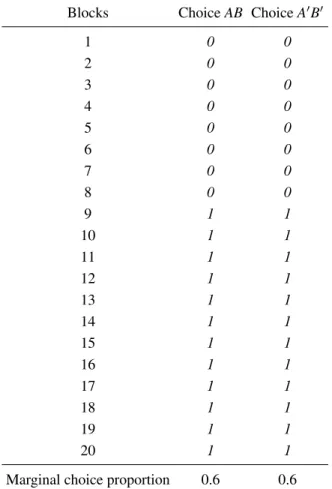
Table 1 shows a hypothetical matrix of responses, where “0” indicates that the person chose alternativeA or A′ and “1” indicates a preference forB or B′. Each
row represents a different block of trials, and the two en-tries within each row represent the responses to the two, separated presentations of the same choice problem in the same block. The marginal choice proportions are the col-umn sums, divided by the number of blocks (20). The two marginal choice proportions are each 0.6.
Let each response combination in a block (row of Table 1) be called aresponse pattern. There are four possible response patterns:00,01,10, and11. In order to be con-sistent within a block, the person had to push opposite buttons on separate trials to indicate preference forAand A′(00), or forBandB′(11).
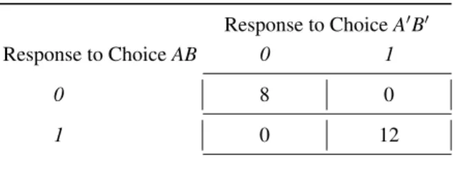
Ifresponse independenceheld, the probability of each response pattern would be given by the product of the marginal probabilities. For these data, the predicted pro-portion for11would be (.6)(.6) = .36, and the predicted proportion of reversals 01 or 10 would be (.4)(.6) + (.6)(.4) = 0.48. However, Table 2 shows that the response patterns do not satisfy independence. Instead, the propor-tion of11was 0.6 (instead of 0.36), and this person was perfectly consistent within blocks (0% reversals, instead of 48%), thereby violating response independence.
By either the Fisher exact test on Table 2, or by means of Birnbaum’s (2012a) test on the variance of preference reversals between blocks (on Table 1), one can reject re-sponse independence withp< .0001. In every case where this person choseA in a block, that same person chose A′ in the same block, and in every block where the
per-Table 1: A hypothetical table of results to responses by the same person to the same choice problem presented twice each in 20 blocks of trials.
Blocks ChoiceAB ChoiceA′B′
1 0 0
2 0 0
3 0 0
4 0 0
5 0 0
6 0 0
7 0 0
8 0 0
9 1 1
10 1 1
11 1 1
12 1 1
13 1 1
14 1 1
15 1 1
16 1 1
17 1 1
18 1 1
19 1 1
20 1 1
Marginal choice proportion 0.6 0.6
son choseB, that person choseB′. This person was
per-fectly consistent within blocks but changed preferences between blocks, resulting in violations of response inde-pendence.
A second, sequential type of violation of iid is also apparent in the Table 1. In particular, this person chose AandA′ on every choice for the first 8 blocks and then
switched to choosingBandB′. Something changed over
trials, resulting in a systematic violation of stationarity within each column. This type of sequential violation is detected by Birnbaum’s (2012a) correlation test, which evaluates the correlation coefficient between the mean number of preference reversals between rows and the gap (in blocks) between rows. In this case, the correlation,r = 0.94, andp< .0001.
Table 2: Data from Table 1 are organized in a cross-tabulation to evaluate independence. These data violate independence, because products of marginal proportions fail to reproduce joint proportions.
Response to ChoiceA′B′
Response to ChoiceAB 0 1
0 8 0
1 0 12
2.2
True-and-error model for One Choice
Problem Repeated in Each Block
A TE model can be expressed for this situation as fol-lows: Suppose that two responses by the same person to the same choice problem within a block are governed by the same “true” preferences, except for random error, and suppose that responses in different blocks might be gov-erned by different “true” preferences (Birnbaum, 2011; Birnbaum & Bahra, 2012a).
Suppose that if the person is in the “true state” of pre-ferringAthe error probability ise, which is the probabil-ity of choosingBwhen the true preference isA. Assume that if the person is in the “true state” of preferringB, that the probability of making an error is alsoe. Suppose that the probability of being in the state of truly preferringBis p. Assume thatpand the error rate,e, are stationary (re-main constant) throughout the study, that errors are mu-tually independent, and thate< ½.1
Do these iid assumptions concerning p and e mean that choice responses are independent, as in the so-called “standard true-and-error model” by Cha et al. (2013)? No, absolutely not. This TE model violates response in-dependence, as shown next.
The predicted probabilities of the four response pat-terns are as follows:
P(00) =p(e)(e) + (1–p)(1–e)(1–e) (1)
P(01) =P(10) =e(1–e) (2)
P(11) =p(1–e)(1–e) + (1–p)(e)(e) (3) P(11) is the predicted probability in the TE model for showing the response pattern11in a block,pis the prob-ability of “truly” preferringBandB′, andeis the
proba-bility of a random error. The marginal choice probaproba-bility of choosingBin a singleABchoice problem is given as follows:P(1*) =P(10) +P(11) =p(1–e) + (1–p)e, where 1More complex models can also be tested (Birnbaum, 2012b; Birn-baum & Schmidt, 2012). For example, it is possible to test models in which error rates depend on a person’s “true” preference state.
P(1*) is the marginal, binary probability of choosingB overA.
Do Equations 1–3 satisfy response independence? That is, can we writeP(11) =P(1*)P(*1)? No. Ifp = .6 ande= 0, for example, this model is perfectly consis-tent with the data of Table 2 that systematically violate response independence.
This violation of response independence by the TE model does not require the error rate to be zero; for ex-ample, ifp= 0.63 ande= 0.11, thenP(1*) =P(*1) = 0.6, soP(1*)P(*1) = 0.36, whereasP(11) = 0.50.
So even though errors are independent of each other, responses are not predicted to be independent, except in special cases, such as whenp= 1. Put another way: even though probability of the conjunction of two errors is rep-resented by the product of their probabilities, the proba-bility of a conjunction of two responses is not given by the product of response probabilities, but instead by Equa-tions 1–3.
Cha et al. (2013, Equation 6) presented a model that satisfies response independence and called it the “stan-dard true-and-error” (STE) model. Independence can hold in special cases of TE, such as when p = 1, but Expressions 1-3 do not satisfy independence in general (Birnbaum, 2011). The Cha et al. STE model is not a standard TE model; instead, it is only a special case in which there is only one true preference pattern; that model is not relevant to this debate, as noted by Birnbaum (2011, p. 680).
Cha et al. (2013, p. 70) next claimed that if a TE model allowed that people changed true preference be-tween blocks (to account for violations of iid), the TE model would become un-testable. That claim is also false, even in this simplest case of a single choice prob-lem, as shown next.
Table 3 displays four different hypothetical cross-tabulations of a repeated choice to show that response in-dependence and error inin-dependence can separately fly or fail; that is, failure or satisfaction of one neither guaran-tees nor refutes the other. (Entries in Table 3 sum to 100, so they can be viewed as percentages, or divided by 100 to facilitate calculations on proportions). Each of these models (independence and TE) can be tested by a Chi-Square on the same 2× 2 array with 1 df, since each model uses two parameters. Response independence im-plies that each cell entry can be reconstructed from the row and column marginal proportions, and TE says that each entry can be reconstructed frompande, using Equa-tions 1-3.
Table 3: Hypothetical cross-tabulations illustrating that response independence and TE independence can be separately satisfied or violated by repeated responses to a single choice problem. Both models are satisfied in the example in the upper left and both are violated in the case in the lower right.
Independence satisfied Independence violated
TE satisfied A′ B′ A′ B′
A 16 24 30 10
B 24 36 10 50
TE violated A′ B′ A′ B′
A 8 32 20 25
B 12 48 5 50
In the two examples of Table 4 that violate response independence, people are more consistent than expected (i.e., the entries on the major diagonal are greater than expected from products of marginal proportions). In the two cases violating TE, the matrices are not symmetric (i.e., one type of preference reversal between replications is more probable than the other).
Treating the hypothetical entries in the tables as ob-served frequencies, theχ2(1) for cases violating
indepen-dence are 34.0 and 16.5 in the first and second rows, re-spectively. Theχ2(1) for examples violating TE are 9.66
and 22.14, respectively. The critical value ofχ2(1) withα
= .01 is 6.63, so each of these would be considered “sig-nificant”. In the two cases satisfying TE, the parameters arep= 1 ande= .4 in the case that also satisfies response independence andp= .63 ande= 0.11 in the case that vi-olates response independence. Chi-Squares are zero for models that fit perfectly.2
These four examples refute the claims by Cha et al. (2013) that the standard TE model implies independence, and they refute the claim that if TE models violated in-dependence, they would be rendered un-testable. See also Birnbaum and Bahra (2012a, pp. 407–408), includ-ing their example in which the TE model would be re-jected.
2In order to justify comparing the calculated Chi-Squares with the Chi-Square distribution to test either response independence or TE in-dependence, higher order independence assumptions would be made; namely, each datum in the table entered its cell independently of the other entries. These higher-order assumptions to justify the significance test do not assume response independence. It is reasonable to question in empirical applications whether or not these higher-order assumptions are satisfied.
2.3
True-and-error model with multiple
subjects and one block each
Now suppose that the data in Table 1 instead represented results from 20differentparticipants, each of whom par-ticipated in only one block (instead of 20 blocks by the same person). That is, suppose each row of Table 1 rep-resents responses by a different person, tested separately. What is the “standard” TE model for that situation? In that case, Equations 1–3 are the same, but the interpre-tations of parameters differ. It is again assumed that the same person in the same block of trials is governed by the same “true” preferences, but in this case, it is assumed that different people might have different “true” prefer-ences. In this case,prepresents the proportion of people who “truly preferredB” in their first (and only) block. In this case, violation of independence arises because differ-ent people have differdiffer-ent “true” preferences.
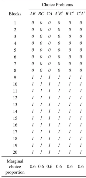
Birn-Table 4: Hypothetical data in a test of transitivity for a single person who receives three choice problems twice in each of 20 blocks of choice problems, where each of the six choice trials was separated by many filler trials and each block of trials was also separated by multiple separator trials.
Choice Problems
Blocks AB BC CA A′B′ B′C′ C′A′
1 0 0 0 0 0 0
2 0 0 0 0 0 0
3 0 0 0 0 0 0
4 0 0 0 0 0 0
5 0 0 0 0 0 0
6 0 0 0 0 0 0
7 0 0 0 0 0 0
8 0 0 0 0 0 0
9 1 1 1 1 1 1
10 1 1 1 1 1 1
11 1 1 1 1 1 1
12 1 1 1 1 1 1
13 1 1 1 1 1 1
14 1 1 1 1 1 1
15 1 1 1 1 1 1
16 1 1 1 1 1 1
17 1 1 1 1 1 1
18 1 1 1 1 1 1
19 1 1 1 1 1 1
20 1 1 1 1 1 1
Marginal choice proportion
0.6 0.6 0.6 0.6 0.6 0.6
baum and Gutierrez (2007) found evidence that this sim-ple model could be rejected in favor of a more comsim-plex model in which different people had different error mul-tipliers.3
IniTET, stability ofemeans that the individual main-tains the same error rate throughout the study, which would be violated in cases where a person becomes better with practice or where she might become fatigued over
3Birnbaum and Gutierrez (2007) also hypothesized that each person might have only a single pattern of “true” preferences; however, their study was not designed to test that conjecture, as this issue is moot in a gTET study. When it was tested by Birnbaum and Bahra (2007b, 2012a, 2012b), this hypothesis was rejected.
trials. It is important to realize that these theorized vio-lations of the model can be tested against more general models that allow the violations of these assumptions.
It is also important to keep in mind that violations of independence in these two cases, as interpreted by the iTET andgTET models come from different origins. So even though the equations are the same, the violations of independence have different empirical interpretations.
For example, the correlation test proposed by Birn-baum (2011, 2012a) is really anticipated to be violated only in the case ofiTET, because that statistic is sensitive to violations of iid that arise from sequential effects; that is, preference reversals between rows that are related to the temporal separation between blocks. If that test were to show significant violations in thegTET paradigm, it would mean that the order in which people were tested somehow affected the results, for example, that partici-pants communicated via some type of ESP that depended on the sequence in which they were tested. Therefore, the data of Table 1 are not realistic for thegTET situa-tion, if the rows represented the order in which different participants were separately tested. A more realistic ex-ample forgTET could be created from Table 1 by ran-domly switching rows, which would create a random se-quence within each column; however, that resorting of rows would preserve the same cross-tabulation as in Ta-ble 2.
At this point, it is also worthy of note that, whereas the results in Table 2 are perfectly consistent withiTET, that model does not allow one to predict nor to fit the sequential information in the data of Table 1. In order to describe the obvious sequential effects in Table 1, one would need additional theory, such as that proposed by Birnbaum (2011, p. 680), and described more fully here in Appendix B. For example, one might theorize that the parameters of a decision making model (such as the TAX model of Birnbaum, 2008) might drift from block to block as in a random walk.
Although one might propose a TE model in which an individual randomly and independently samples a pref-erence pattern in each block of trials, I doubt that such a model would be an accurate descriptive model, based on the findings with the correlation tests on data of Birn-baum and Bahra (2012b) and of Regenwetter et al. (2011) as analyzed in Birnbaum (2012a).
Cha et al. (2013, p. 68) made a peculiar argument about the relation between these two cases as follows: First, they claimed that iTET models imply indepen-dence. (They do not.) Second, they argued that, if Birn-baum and Bahra (2012b) found violations of indepen-dence within a person (which they did), it would inval-idate the between-subjects model of Birnbaum and Bahra (2007a), which it would not. The model in the 2007a paper was agTET model that violates iid because of in-dividual differences. In essence, Cha et al. argued that if iid is violated in the case ofiTET it means thatgTET is rendered “untenable”. That is neither logical nor reason-able.
One might plausibly argue just the opposite; namely, if individuals change true preferences from block to block, it seems likely that people would also differ from each other. Therefore, evidence of violations of iid in theiTET case (Birnbaum & Bahra, 2012b) would seem from com-mon sense to suggest that oneshouldexpect to find viola-tions of iid in thegTET case (Birnbaum & Bahra, 2007a). But keep in mind that neither iTET nor gTET sat-isfy iid and there is noa priori connection between the two. That is, violations of iid in one neither guarantees nor rules out violations of iid in the other case. For ex-ample, it is logically possible (if intuitively implausible) that, although each person might change true preferences from block to block, all humans might go through such changes in the same exact sequence.
Empirical results show that neither between-subjects data of Birnbaum and Bahra (2007a) nor the within sub-jects data of Birnbaum and Bahra (2007b, 2012a, 2012b) satisfied independence. Neither theiTET norgTET mod-els used in those studies implies independence. Further, empirical intuition leads one to anticipate that if iid is vi-olated in theiTET case, one should expect to find vio-lations in thegTET case. So, the claims by Cha et al. (2013, p. 68) that violations of iid in Birnbaum and Bahra (2012b) render thegTET model of Birnbaum and Bahra (2007a) “not tenable” is not correct.
The violation of response independence is the main is-sue in this debate, which is that such violations could lead to wrong conclusions concerning transitivity, if a person analyzed only marginal choice proportions. The assump-tion of iid is not merely some statistical nicety that justi-fies significance tests; violations mean that the interpreta-tion of marginal proporinterpreta-tions can be misleading, as shown in the next section.
3
Testing independence, TE
mod-els, and transitivity
Transitivity of preference asserts that, ifAis preferred to BandBis preferred toC, thenAshould be preferred toC.
To test this principle, we need at least three choices. To test TE models for this case, each of these three choices can be repeated within each block. So, this new experi-mental setup is like the previous one, except that within each block of choice problems, there are three choice problems that are each repeated within each block; these six problems are spaced out by multiple fillers, and blocks are separated as before.
3.1
Three choices repeated twice in each
block
Suppose there are three choice problems: AB,BC, and CA. Let ChoiceA′B′represent a second version of theAB
choice that might require the person to switch buttons in order to indicate the same preference response. Choices B′C′andC′A′are similarly constructed.
Again, let us start with the paradigm of a single partici-pant who serves in 20 blocks of trials that include six sep-arated choice problems: 3 basic choice problems repeated within blocks, with all choices separated by intervening fillers, and blocks separated by numerous separators. Hy-pothetical data are shown in Table 4.
Data are coded so that000is the intransitive response pattern of choosingAoverB,BoverC, andCoverA. The pattern111represents the intransitive cycle of choosing BoverA,CoverB, andAoverC. The other six response patterns are transitive.
In Table 4 we see that the participant had perfectly intransitive response patterns within every single block of the study. The person began with the intransitive cy-cle 000and switched to the opposite intransitive cycle, 111. Weak stochastic transitivity is violated in the binary choice proportions, becauseP(B ≻ A)> ½,P(C≻B) > ½ andP(A≻C)> ½. Yet the marginal choice propor-tions (0.6, 0.6, 0.6) are perfectly consistent with a mixture of linear orders, satisfying the triangle inequality,P(AB) + P(BC) + P(CA)≤2. If an investigator analyzed only marginal choice proportions, the conclusion from the tri-angle inequality would be that transitivity can be retained. By examining response patterns, however, it is easy to see that every individual response pattern was intransitive.
Cha et al. (2013, pp. 66–68) conceded this point, but they claimed that the TE models would also fail to detect intransitivity in such cases. However, that claim depends on their assumption that the TE model satisfies indepen-dence, which it does not.
The response patterns from Table 4 are cross-tabulated in Table 5. Table 5 is perfectly consistent withiTET in this case, which can violate response independence.
Table 5: Analysis of response patterns from hypothetical data of Table 4.
Response pattern
Observed ABC
Observed A′B′C′
Observed both
Predicted ABC(iid)
Predicted both (iid)
000 8 8 8 1.28 .08
001 0 0 0 1.92 .18
010 0 0 0 1.92 .18
011 0 0 0 2.88 .41
100 0 0 0 1.92 .18
101 0 0 0 2.88 .41
110 0 0 0 2.88 .41
111 12 12 12 4.32 .93
Sum 20 20 20 20 2.81
0.6, the total probability that a response pattern will be re-peated within blocks is only 0.14; so out of 20 trials, the person is expected to agree in choice pattern only 2.81 times within blocks. In these hypothetical data, however, the participants were perfectly consistent (20 agreements = 100%). Do real data show higher self-consistency than predicted by independence? They do (Birnbaum & Bahra, 2012a, Footnote 4; Birnbaum & Bahra, 2012b, Appendix H).
The examples in Birnbaum (2012a), like that in Ta-ble 5, are cases where the cross-tabulations are perfectly consistent with TE models and error rates are zero. Per-haps these perfect features of the examples led Cha et al. (2013, p. 70) to state that, if TE models are allowed to violate iid, they always fit perfectly and are therefore not testable. The next sections show the appropriate TE models for testing transitivity in the presence of error, and illustrate cases where the TE model leads to different con-clusions from those reached by the methods used by Re-genwetter et al. (2011). Examples where TE models can be rejected are also presented.
3.2
True-and-error model for Test of
Tran-sitivity
There are 8 possible response patterns for each test with three choice problems testing transitivity:000,001,010, 011, 100, 101, 110, and 111. In the TE model, the predicted probability of showing the intransitive pattern, 111, is given as follows:
P(111) =p000(e1)(e2)(e3) +p001(e1)(e2)(1 –e3)
+p010(e1)(1 –e2)(e3) +p011(e1)(1 –e2)(1 –e3)
+p100(1 –e1)(e2)(e3) +p101(1 –e1)(e2)(1 –e3)
+p110(1 –e1)(1 –e2)(e3)
+p111(1 –e1)(1 –e2)(1 –e3). (4)
P(111) is the theoretical probability of observing the in-transitive response cycle of 111; p000, p001, p010, p011, p100, p101, p110, and p111 are the probabilities that the
person has these “true” preference patterns, respectively (these 8 terms sum to 1);e1,e2, ande3are the
probabili-ties of error on theAB,BC, andCAchoices, respectively. These error rates are assumed to be mutually indepen-dent, and each is less than ½.
There are seven other equations like Equation 4 for the probabilities of the other seven possible response pat-terns.
Because each choice is presented twice in each block, there are 64 possible response patterns for all six re-sponses within each block. If error rates are assumed to be the same for choice problemsA′B′, B′C′, and C′A′
as for choice problemsAB,BC, andCA, respectively, the probability of showing the same pattern,111, on both ver-sions in a block is the same as in Equation 4, except each of the error terms,eor (1 –e) in Equation 4 are squared. In this way, one can write out 64 expressions for all 64 possible response patterns that can occur in one block.
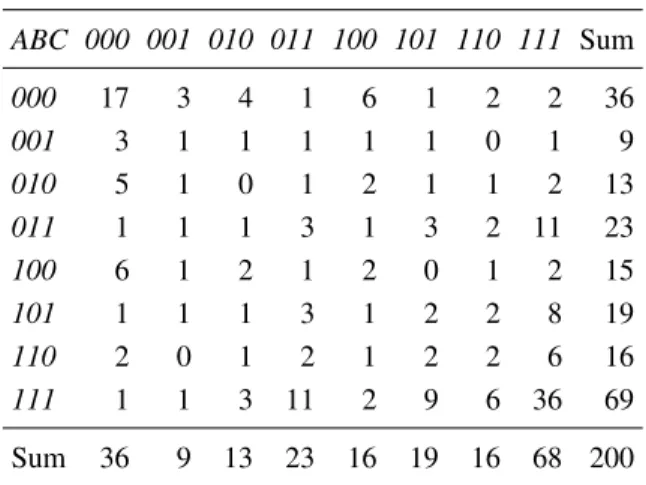
A hypothetical set of data is shown in Table 6. The rows show the 8 possible response combinations for the ABC choices and the columns show the 8 possible re-sponse patterns for the A′B′C′ choices. Each entry is
the frequency with which each response pattern occurred. For example, the 17 in the first row and column shows that on 17 out of 200 blocks, the person showed the in-transitive pattern,000, in both versions of the three choice problems.
ThegeneralTE model for this case has 8 parameters for the 8 “true” probabilities and 3 error rates (one for each choice problem).4 Because these 8 “true”
Table 6: Hypothetical data containing error that illustrate testing independence, TE model, and transitivity. Analy-ses described in the text show that these data violate in-dependence, they satisfy TE model, and they violate tran-sitivity.
Response Pattern inA′B′C′choices
ABC 000 001 010 011 100 101 110 111 Sum
000 17 3 4 1 6 1 2 2 36
001 3 1 1 1 1 1 0 1 9
010 5 1 0 1 2 1 1 2 13
011 1 1 1 3 1 3 2 11 23
100 6 1 2 1 2 0 1 2 15
101 1 1 1 3 1 2 2 8 19
110 2 0 1 2 1 2 2 6 16
111 1 1 3 11 2 9 6 36 69
Sum 36 9 13 23 16 19 16 68 200
ities sum to 1, they use 7 df, so the model uses 10 df to account for 64 frequencies of response patterns; the data have 63 df because they sum to the total number of blocks. It should be clear that there are many ways for 64 frequencies to occur that are not compatible with a model with 11 parameters. Two examples will be pre-sented later.
ThetransitiveTE model is a special case of this gen-eral TE model in which the two probabilities of intran-sitive patterns are set to zero, p000 = p111 = 0. If the
error rates are not zero, a set of data can (and typically would) still show some instances of intransitive response patterns, even though the “true” probabilities of these pat-terns are each zero.
One can conduct at least three types of statistical tests. First, one can test independence. Second, one can test this general TE model. Third, if the general TE model pro-vides a reasonable approximation, one can test the special case of transitivity within that model.5
According to response independence, it should be pos-sible reproduce the entries in Table 6 from just three num-bers: the marginal choice proportions,P(AB),P(BC), and P(CA). These are all 0.6, so the predicted entry for the up-per left cell of Table 6 (000,000) would be [1 –P(AB)]2[1
–P(BC)]2[1 –P(CA)]2= (.4)6 = 0.004. Multiplying by
the total frequency (200), the predicted frequency is 0.82, far less than the observed value of 17.
For an overall index of fit, one can compute
transitivity.
5An Excel spreadsheet that implements these analyses is available with this article.
χ2=Σ(f
i– Fi)2/Fi. Wherefiare the observed
frequen-cies andFiare the corresponding predicted frequencies,
based on independence (or below, predicted from the TE model). There are 63 df in the data, and we used 3 df to estimate the three parameters (the marginal choice pro-portions), so this test of independence has 60 df. In this case, χ2(60) = 505.4, so the conclusion would be that these data do not satisfy response independence.6
Next, one can use a function minimizer, such as the solver in Excel, to estimate best-fit parameters for the general TE model. Those estimates arep000= .333,p111=
.667,p001=p010=p011=p100=p101=p110= 0;e1= 0.25,
e2= 0.20, ande3= 0.15. In this case, 10 df were used to
estimate the parameters, andχ2(53) = 11.5, showing that the general TE model fits these hypothetical data well.
However, when we fixp000=p111= 0, in order to test
the transitive special case, and solve for the best-fit pa-rameters, we find that the transitive TE model does not fit these data,χ2(55) = 108.3. The difference,χ2(2) = 108.3
– 11.5 = 96.8, indicates that transitivity is not satisfactory as a description of these same data.
These calculations show that, in principle, one can es-timate the models and assess their fit in the 8×8 ma-trix as in Table 6. In practice, however, it might be diffi-cult or impractical to obtain sufficient data for such a full analysis. When the data are thinner, one might partition the data in various ways and still test independence, TE model, and transitivity, as described next.
3.3
Partitions of the data
In order to test independence to compare the iid models with TE models, one might partition the data from the 8× 8 matrix (as in Table 6) into three, 2×2 matrices, in order to test the models of repetitions, as was done in Tables 2 and 3. For example, one can tabulate theABchoice by theA′B′ choice. From Table 6, the four frequencies are
44, 37, 37, and 82, for 00, 01, 10, and 11, respectively. These violate independence by a standard chi-square test, χ2(1) = 10.8. However, the same values fit the TE model,
χ2(1) = 0.2, with e
1 = 0.25. Similarly, the tabulations
for the other two choice problems also violate response independence,χ2(1) = 20.7 and 40.3, and also satisfy TE
independence,χ2(1) = 0.1, and 0.5, withe
2= 0.2, ande3
= 0.15, respectively. Because these error estimates do not assume or imply the property of transitivity, they might be used to constrain solutions to other partitions of the data that can be used to test transitivity.
6Another index of fit is theG-squared statistic, which arises as a maximum likelihood,G2= -2Σln(f
i/Fi), which is considered a better
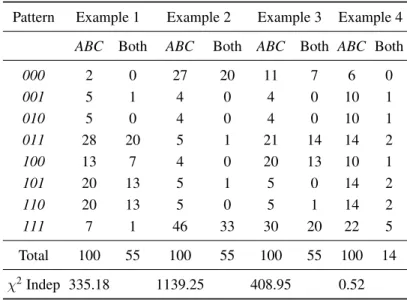
Table 7: Hypothetical examples testing transitivity; these examples illustrate use of partitioned data to compensate for small sample sizes. Marginal choice proportions are the same in all examples. Examples 1-3 violate iid. Example 1 satisfies transitivity, which is violated in Examples 2 or 3. Frequencies under “ABC” represent response patterns to ChoiceAB,BC, andCA, so000and111are intransitive; frequencies under “Both” indicate the same response pattern repeated within blocks. Example 4 satisfies iid model of Regenwetter et al. (2011), which wrongly concludes that all four of these examples satisfy transitivity.
Pattern Example 1 Example 2 Example 3 Example 4
ABC Both ABC Both ABC Both ABC Both
000 2 0 27 20 11 7 6 0
001 5 1 4 0 4 0 10 1
010 5 0 4 0 4 0 10 1
011 28 20 5 1 21 14 14 2
100 13 7 4 0 20 13 10 1
101 20 13 5 1 5 0 14 2
110 20 13 5 0 5 1 14 2
111 7 1 46 33 30 20 22 5
Total 100 55 100 55 100 55 100 14
χ2Indep 335.18 1139.25 408.95 0.52
A useful partition for testing transitivity is to count the frequencies of the 8 possible response patterns in theAB, BC, andCAchoices and the frequencies of repeating the same patterns on both ABC and A′B′C′ choices within
blocks. These values can be found in the row sums of Table 6 and on the major diagonal, respectively. But these frequencies contain cases in common, so they are not mutually exclusive. One can construct a mutually ex-clusive, exhaustive partition by counting the frequency of showing each pattern on both repetitions of the same choice problems and the frequency of showing each of 8 response patterns in the ABCchoices and not in both cases. For example, in Table 6, the frequency of showing the 000 pattern in theABC choice problems and not in both forms is 36–17 = 19.
This partition of the data reduces the 64 cells as in Ta-ble 6 to 16 cells. This partition has the effect of increas-ing the frequencies in each cell, but reducincreas-ing the degrees of freedom in the test. In this partition, we can also test independence, TE model, and transitivity. The purpose of the partition is to increase the frequencies within each cell, in order to meet the assumptions of the Chi-Square orG-Square statistical tests.
Four examples of hypothetical data are shown in Ta-ble 7 to illustrate different cases that might be observed with this type of partition. The numbers have been cho-sen to sum to 100 so that they could be easily converted to proportions to facilitate calculations for the models.
All four examples in Table 7 have identical marginal
choice proportions, so any method of analysis that fo-cused strictly on marginal choice proportions treats these four examples as identical, but they are quite differ-ent from each other. The marginal choice proportions, P(AB),P(BC), andP(CA) are all 0.6, so these examples all violate weak stochastic transitivity, and all satisfy the triangle inequality. However, they have different interpre-tations, as shown below.
These response patterns are listed in terms of theABC choice pattern and repeated patterns. To convert to a mutually exclusive and exhaustive partition, subtract the “both” frequencies from the ABC frequencies, as de-scribed above. The Chi-Squares are then computed in the conventional way comparing observed frequencies with those predicted by the models.
First, we can test independence, which is the assump-tion that products of marginal choice proporassump-tions cor-rectly reproduce all 16 cells in this partition of the data. Three parameters (three marginal choice proportions) are calculated from the data, leaving 15 – 3 = 12 df for the test of independence. The critical value ofχ2(12) with
α= .01 is 26.22. The last row of Table 6 shows these χ2tests; only Example 4 satisfies independence.
Table 8: Best-fit solutions of TE models to Example 2 of Table 7. These hypothetical data satisfy the triangle inequality yet are perfectly intransitive, according to the fit of the TE models. Fixed values are shown in parentheses and constrained values are shown in brackets. Constrained errors are estimated strictly from preference reversals to the same choice problem within blocks, using the three, 2×2 partitions as in Table 3.
Unconstrained errors Constrained errors
Parameter General Transitive Intransitive General Transitive Intransitive
p000 0.378 (0) 0.378 0.378 (0) 0.375
p001 0.000 0.342 (0) 0.000 0.141 (0)
p010 0.000 0.045 (0) 0.000 0.116 (0)
p011 0.011 0.000 (0) 0.011 0.184 (0)
p100 0.000 0.030 (0) 0.000 0.116 (0)
p101 0.011 0.015 (0) 0.011 0.184 (0)
p110 0.000 0.568 (0) 0.000 0.259 (0)
p111 0.600 (0) 0.622 0.601 (0) 0.625
e1 0.095 0.024 0.112 [0.1] [0.1] [0.1]
e2 0.095 0.024 0.112 [0.1] [0.1] [0.1]
e3 0.103 0.500 0.091 [0.1] [0.1] [0.1]
χ2 1.98 88.48 3.29 2.02 4194.97 3.67
That leaves 5 df to test the model in this partition.7 Third, if the TE model fits, we can test the transitive model by fixing the values of p000 = p111 = 0, which
means that the solution is restricted to be purely transi-tive. The difference in fit between the general case where probabilities of all “true” patterns are free and the transi-tive special case provides a test of transitivity on 2 df.
Example 1 of Table 7 violates independence [χ2(12)
= 335.18]; however, it satisfies both the TE model and transitivity. The TE model fit these data with error rates constrained to match the preference reversals data only, where e1 = e2 = e3 = 0.1, where p000 = p111 = 0 were
fixed, and where the best-fit solution yielded p001 = 0, p010= 0,p011= 0.325,p100= 0.125,p101= 0.25, andp110
= 0.25. This model hasχ2 = 2.04, so it should be clear
that there is no room for a significant improvement by making the model more complex. So this case violates iid, but satisfies the TE model and transitivity.
However, Example 2 is a very different case from Ex-ample 1, as shown in Table 8. Six models have been fit to those data, including the general TE model (all 8 response patterns allowed), the transitive special case (both intran-sitive patterns are fixed to zero), and a purely intranintran-sitive model (only intransitive patterns are allowed). Parame-ters shown in parentheses are fixed, and those shown in square brackets are constrained.
7We also had opportunities to reject the TE model via the three, 2× 2 cross-tabulations of repeated choices.
When the general TE model fits the data, one might constrain the error rates in this analysis to agree with values estimated strictly from replications data (from the three, 2×2 cross-tabs). The constrained version provides greater power for the test of transitivity.
The fact that the TE general model fits either with or without constrained errors shows that we can retain the general TE model. The differences in Chi-Squares be-tween the general model and the transitive special case are large enough to reject the transitive model either with or without constrained errors (χ2(2) = 4192.95 and 86.50, respectively). The purely intransitive special case also fits these data acceptably because the difference in Chi-Squares between the general model and purely intransi-tive model is not significant in either constrained or free cases.
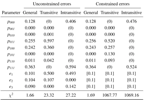
Table 9 shows the corresponding analyses for Exam-ple 3. The general TE model is again acceptable with or without constrained errors. In this case, however, both the purely transitive model and the purely intransitive model can be rejected. Therefore, one would conclude that these data are best represented as a mixture of transitive and in-transitive response patterns.
Table 9: Fit of TE models to Example 3 of Table 7. These hypothetical data satisfy the triangle inequality but they contain a mixture of transitive and intransitive response patterns. Neither the purely transitive nor purely intransitive solutions yields an acceptable fit.
Unconstrained errors Constrained errors
Parameter General Transitive Intransitive General Transitive Intransitive
p000 0.128 (0) 0.406 0.128 (0) 0.476
p001 0.000 0.000 (0) 0.000 0.000 (0)
p010 0.000 0.001 (0) 0.000 0.000 (0)
p011 0.255 0.597 (0) 0.256 0.520 (0)
p100 0.242 0.360 (0) 0.243 0.257 (0)
p101 0.000 0.000 (0) 0.000 0.130 (0)
p110 0.011 0.042 (0) 0.011 0.093 (0)
p111 0.363 (0) 0.594 0.364 (0) 0.524
e1 0.101 0.500 0.493 [0.1] [0.1] [0.1]
e2 0.104 0.107 0.000 [0.1] [0.1] [0.1]
e3 0.090 0.000 0.142 [0.1] [0.1] [0.1]
χ2 1.66 23.32 27.22 1.69 1067.77 1069.16
with transitivity, as would all of these examples. In the approach of Regenwetter et al. (2011), no statistical test would be conducted because the model “fits perfectly” in all of these cases.
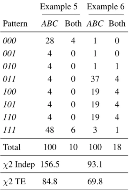
Table 10 provides two hypothetical examples showing that the TE model need not always fit. Marginal choice proportions in Examples 5 and 6 are the same as in Ex-amples 1–4 of Table 7. In both cases iid is violated, but in both cases the general TE model fails. In Example 5, the response patterns observed are mostly intransitive and in Example 6 most of the response patterns observed are transitive.
To understand what went wrong for the TE models in these examples, recall that errors are assumed to be mutu-ally independent. Although TE models violate indepen-dence of responses, they satisfy indepenindepen-dence of errors, and the errors in these examples violate that assumption. In these examples, the participant was not completely consistent so errors are not zero; we know that there are substantial errors because people did not repeat the same response patterns in both versions very often. But if er-rors are not zero and are mutually independent, we should have observed more instances of response patterns 001, 010, 100, 011, 100, 101, and 110 in Example 5, and yet too few such cases are observed. Instead, whenever a per-son made an error on one choice problem, they too often made an error on other choice problems. Example 6 also violates TE because data violate independence of errors. Examples 5 and 6 violate iid and violate TE model.
In summary, one can separately test independence, TE,
and transitivity. These examples illustrate how the TE model can be applied and they refute the claims by Cha et al. (2013) that TE models must satisfy response inde-pendence or become vacuous.
Difficulties in the approach of Regenwetter et al. (2011) are illustrated by these examples. Based on marginal choice proportions, all of these examples are the same and all are perfectly consistent with transitiv-ity. When we examine the data as in Tables 6-10, we see that some cases systematically violate iid and among those, some cases systematically violate transitivity and others satisfy it. When iid assumptions are satisfied, then marginal choice proportions contain all of the useable in-formation in the data, but when iid is violated, we need to examine response patterns to correctly diagnose the sub-stantive issue of transitivity.
These hypothetical examples illustrate why it is im-portant to know whether iid assumptions, especially re-sponse independence, are empirically satisfied in choice experiments. Birnbaum and Bahra (2007b, 2012b) found that iid was violated in a series of experiments testing transitivity. Birnbaum’s (2012a) reanalysis of Regenwet-ter et al. (2011) also concluded that iid was not satisfied for those data.
Table 10: Hypothetical examples violating both response independence and the TE model with all parameters free. As in Table 7, these examples have the same marginal choice proportions (all 0.6).
Example 5 Example 6
Pattern ABC Both ABC Both
000 28 4 1 0
001 4 0 1 0
010 4 0 1 1
011 4 0 37 4
100 4 0 19 4
101 4 0 19 4
110 4 0 19 4
111 48 6 3 1
Total 100 10 100 18
χ2 Indep 156.5 93.1
χ2 TE 84.8 69.8
other tests of “iid” were satisfied “with flying colors” for the Regenwetter et al. (2011) data. Each of these claims is refuted in Appendix A, where it is shown that the evi-dence against iid is significant in all three sets of data re-viewed by Cha et al., that thep-values estimated by Birn-baum’s methods are conservative relative to the method used by Cha et al., and that the tests of “iid” that were not significant “with flying colors” in Cha et al. do not test response independence.
3.4
Birnbaum and Bahra data violate iid
Birnbaum and Bahra (2007b, 2012b) also used three de-signs for each participant in each study; they used 136 participants (in three studies) compared to 18 in Regen-wetter et al. (2011) and they asked each person to respond twice to each choice problem in each block (compared to once per block in Regenwetter et al., 2011). They also used a greater variety of choice problems that might be expected to create more interference in memory, and blocks were properly separated by numerous interven-ing tasks. Therefore, this 2012b paper with 136 partic-ipants must be accorded corresponding greater weight in relation to a study with only 18 participants. As shown in Birnbaum and Bahra (2012b), evidence against iid in those studies was extremely strong.
Birnbaum and Bahra (2007b, 2012b) found that a num-ber of participants completely reversed preferences for 20 out of 20 choice problems between blocks; this
pro-vides a clear refutation of the theory of iid. Because each block of each design in that study contained 20 exper-imental choice problems (excluding fillers and separa-tors), a complete reversal has a probability of ½ to the 20thpower, assuming iid, which is less than one in a
mil-lion. There were 18 people out of 136 who showed at least one such perfect reversal of 20 out of 20 responses between blocks, and these 18 produced hundreds of in-stances of such perfect reversals. In fact, one person re-versed preferences perfectly between 60 choice problems (all three designs) between blocks (see Table 2 of Birn-baum & Bahra, 2012b). These and other analyses of those data show that iid can be rejected.
4
Discussion
In my opinion, the empirical results obtained so far tell us that any viable approach to analyzing formal properties in choice data should be able to handle the possibility that the assumptions of response independence is violated. It should allow for the possibility that people behave more consistently than allowed by the simplifying assumptions of iid. The TE models can handle certain violations of response independence. These models do not satisfy re-sponse independence and yet they are testable because they cannot handle all such violations.
As shown in the examples presented here, TE model can distinguish and diagnose cases that look identical to tests defined on marginal choice proportions (such as weak stochastic transitivity and the triangle inequality). All of the examples in Tables 6, 7, and 10 have the same binary choice proportions. However, I think it proper to conclude that Example 1 of Table 7 satisfies transitivity and that Examples 2 and 3 in Table 7 violate it. Example 4 satisfies iid and is therefore open to debate, because a person might have a mixture that is purely transitive or might have a mixture including intransitive patterns and still produce such data.
These different conclusions for these different exam-ples could not be reached by examination of the marginal choice proportions alone, because they all have the same marginal proportions. My advice to those testing transi-tivity or other properties is that they should analyze data at the level of response patterns rather than at the level of marginal choice proportions.
4.1
Are criticisms of using marginal
pro-portions dependent on the TE model?
choice proportions applies to any case in which iid is vio-lated, whether those violations satisfy a TE model or not. As shown in Examples 5 and 6 of Table 10, data might violate iid and also violate the TE model. These exam-ples, including those in Table 3, show that the assumption of independence of errors is a testable property of these models, but it is not the same as response independence.
One could argue that TE models are only approximate because they allow that a person can change “true” pref-erences between blocks but not within a block. A more accurate or more general model might allow that a person might change “true” preferences at any point during the study. Such a model would include the iid model used by Regenwetter et al. (2011) and TE models as special cases. According to the model used by Regenwetter et al. (2011), independence is supposed to hold on every experimental trial, as long as there are three filler trials separating experimental trials.
4.2
What if TE models are wrong or
incom-plete?
The TE Models are testable and they might be rejected when appropriate studies have been done. A test ofiTET requires a larger quantity of data from each participant to conduct a proper analysis, whereas tests ofgTET require a large numbers of participants, each of which might con-tribute a smaller amount of data. Whereas a number of experiments in thegTET paradigm have been published, we do not yet have experimental results comparable to the hypothetical Table 6 for theiTET case, and one might reasonably wish for even more data than described in that example.
Although TE models can allow different error rates in different choice problems, and although more general versions can be tested in which different people might have different amounts of noise in their data, even these more general TE models do not provide any fundamental explanation for the sources of the errors.
Nor do TE models proposed so far provide an expla-nation for the kinds of sequential effects that might arise from a process such as described by Birnbaum (2011), in which the parameters of a model of risky decision mak-ing change systematically from trial to trial, as elaborated in Appendix B. Therefore, although TE models provide a testable framework within which issues of independence and transitivity can be explored, they do not provide spe-cific or satisfying answers to important deeper questions. Appendix B shows how sequential models might account for violations of iid including response independence as well as violations detected by the correlation test of Birn-baum (2011, 2012a). These models allow that parameters representing probability weighting or risk aversion might
fluctuate from block to block, but they do not identify the causes of changing parameter values.
But it is important to realize that even if TE models are wrong, as in Examples 5 and 6 of Table 9, or if they are approximate, incomplete or even misguided, criticism of TE models does not mitigate the problems of assuming iid as a basis for testing transitivity. The key problem is that when iid is violated, analysis of marginal choice proportions can easily lead to wrong conclusions.
4.3
Are assumptions of iid only used to
jus-tify statistical tests?
It might be argued that because the assumptions of iid are used to justify statistical tests, that this is their only role in the approach of Regenwetter et al. (2011). That is not true: in fact, it is the assumption of iid that justifies analysis of marginal choice proportions. As shown in the examples of Table 6 and 7, when iid is violated, marginal choice proportions might satisfy the triangle inequality despite systematic violations of transitivity within blocks, revealed in the response patterns.
The statistical issue (that violations of iid affect thep -value of a significance test) is far less important, in my opinion, than the danger of drawing wrong descriptive, substantive conclusions concerning a theoretical property (such as transitivity) from marginal choice proportions. Indeed, when the triangle inequalities are satisfied, as they are in all of the examples analyzed here, the Regen-wetter et al. (2010, 2011) approach conducts no statistical test at all, because the model is said in all of such cases to fit “perfectly”. For example, in Table 7 the triangle in-equality can be “perfectly” satisfied in a case in which a different, deeper analysis (Table 8) would refute any mix-ture of transitive patterns in favor of a mixmix-ture of purely intransitive patterns.
There is another distinction that might be helpful to eliminate some confusion in this dispute. The random preference model used by Regenwetter et al. (2011) al-lows any set of preference patterns to be in the “mind” of the participant. These hypothesized preference patterns can violate independence. Indeed, in the linear order, no intransitive patterns are allowed, so it might seem that this model violates a type of independence in the postulated mental set.
Regenwetter et al. (2011) have pointed out that it is not possible to recover the distribution of true preference patterns from the choice responses of a person, because the assumed independence of responses means that overt responses do not permit recovery of the distribution of preference patterns in the mind of the participant.
The assumption of response independence thus justi-fies analysis of marginal choice proportions, while it also makes it impossible to identify the distribution of the-orized preference patterns. When iid is assumed, one might, in principle, reject transitivity in this approach, but one cannot recover the distribution of “true” response pat-terns in this model nor can one definitively rule out mix-tures containing intransitive response patterns when the marginal means satisfy transitivity. As shown here, when iid is violated, satisfaction of the triangle inequality can co-exist with systematic violations of transitivity.
The statistical tests used here to illustrate analyses in the TE model also make independence assumptions, but these do not assume nor imply response independence. Obviously, these higher order assumptions might be em-pirically wrong. But if and when the model is appropri-ate, it can be used to estimate the distribution of “true” response patterns.
4.4
The details are in the data
The question of how much detail should be analyzed in data arises in all research problems. The analyses of the various partitions of the data here should clarify that whenever data are aggregated, information can be lost. This debate can be viewed as a debate of how much use-ful information is contained in data and how much detail should be represented by a model.
For example, there are 20×6 = 120 Values in Table 4. In a larger experiment, there might be a hundred rows. Such a table of data might be summarized by 3 binary choice proportions, by 6 column proportions, by 3, 2×2 cross-tabulations of repeated responses, by 8 proportions of showing each response pattern involving three choice problems, by 8×2 proportions showing each response pattern on the ABC choice (but not both) and in both ver-sions, by the 8×8 cross-tabulation of the eight response patterns in the ABC×A′B′C′repetitions, or at the level
of the original data.
When response independence is violated, as appears to be the case for all three sets of data in Regenwetter et al. (2011) as well as the series of studies in Birnbaum and Bahra (2012b), it means that marginal choice proportions do not tell the whole story. As shown here, response inde-pendence and error indeinde-pendence are different properties, but both properties can be tested, and I think it would be a true error not to test them both.
References
Birnbaum, M. H. (2004). Tests of rank-dependent utility and cumulative prospect theory in gambles represented by natural frequencies: Effects of format, event fram-ing, and branch splitting.Organizational Behavior and Human Decision Processes, 95, 40–65.
Birnbaum, M. H. (2008). New paradoxes of risky deci-sion making.Psychological Review, 115, 463–501. Birnbaum, M. H. (2011). Testing mixture models of
tran-sitive preference: Comment on Regenwetter, Dana, and Davis-Stober (2011). Psychological Review, 118, 675–683.
Birnbaum, M. H. (2012a). A statistical test of the as-sumption that repeated choices are independently and identically distributed. Judgment and Decision Mak-ing, 7, 97–109.
Birnbaum, M. H. (2012b). True and error models of re-sponse variation in judgment and decision tasks. Work-shop on Noise and Imprecision in Individual and Inter-active Decision-Making, University of Warwick, U.K., April, 2012.
Birnbaum, M. H., & Bahra, J. P. (2007a). Gain-loss sepa-rability and coalescing in risky decision making. Man-agement Science, 53, 1016–1028.
Birnbaum, M. H., & Bahra, J. P. (2007b). Transitivity of preference in individuals.Society for Mathematical Psychology Meetings, Costa Mesa, CA. July 28, 2007. Birnbaum, M. H., & Bahra, J. P. (2012a). Separating re-sponse variability from structural inconsistency to test models of risky decision making.Judgment and Deci-sion Making, 7, 402–426.
Birnbaum, M. H., & Bahra, J. P. (2012b). Testing tran-sitivity of preferences in individuals using linked de-signs.Judgment and Decision Making, 7, 524-567. Birnbaum, M. H., & Gutierrez, R. J. (2007). Testing
for intransitivity of preference predicted by a lexico-graphic semiorder. Organizational Behavior and Hu-man Decision Processes, 104, 97–112.
Birnbaum, M. H., & LaCroix, A. R. (2008). Dimension integration: Testing models without trade-offs. Orga-nizational Behavior and Human Decision Processes, 105, 122–133.
Birnbaum, M. H., & Schmidt, U. (2008). An experimen-tal investigation of violations of transitivity in choice under uncertainty. Journal of Risk and Uncertainty, 37,77–91.
Birnbaum, M. H., & Schmidt, U. (2012). Constant con-sequence paradoxes of Allais: Coalescing, restricted branch independence, or error? Foundations of Utility and Risk XV (FUR XV),Atlanta, July, 2012.
Cha, Y., Choi, M., Guo, Y., Regenwetter, M., & Zwill-ing, C. (2013). Reply: Birnbaum’s (2012) statistical tests of independence have unknown Type-I error rates and do not replicate within participant. Judgment and Decision Making, 8, 55–73.
Conlisk, J. (1989). Three variants on the Allais example. American Economic Review, 79, 392–407.
Harless, D. W., & Camerer, C. F. (1994). The predictive utility of generalized expected utility theories. Econo-metrica, 62, 1251–1289.
Lichtenstein, S., & Slovic, P. (1971). Reversals of prefer-ence between bids and choices in gambling decisions. Journal of Experimental Psychology, 89, 46–55. Loomes, G., & Sugden, R. (1998). Testing different
stochastic specifications of risky choice. Economica, 65, 581–598.
Loomes, G., Starmer, C., & Sugden, R. (1991). Observ-ing violations of transitivity by experimental methods. Econometrica, 59, 425–439.
Regenwetter, M., Dana, J. & Davis-Stober, C. (2010). Testing transitivity of preferences on two- alternative forced choice data. Frontiers in Psychology, 1, 148. http://dx.doi.org/10.3389/fpsyg.2010.00148.
Regenwetter, M., Dana, J., & Davis-Stober, C. P. (2011). Transitivity of preferences. Psychological Review, 118, 42–56.
Regenwetter, M., Dana, J., Davis-Stober, C. P., and Guo, Y. (2011). Parsimonious testing of transitive or intran-sitive preferences: Reply to Birnbaum (2011). Psycho-logical Review, 118, 684–688.
Smith, J. B., & Batchelder, W. H. (2008). Assessing in-dividual differences in categorical data. Psychonomic Bulletin & Review,15, 713-731. http://dx.doi.org/10. 3758/PBR.15.4.713.
Sopher, B., & Gigliotti, G. (1993). Intransitive cycles: Rational choice or random error? An answer based on estimation of error rates with experimental data. The-ory and Decision, 35, 311–336.
Tversky, A. (1969). Intransitivity of preferences. Psycho-logical Review, 76, 31–48.
Wilcox, N. T. (2008). Stochastic models for binary dis-crete choice under risk: A critical primer and econo-metric comparison. Research in Experimental Eco-nomics, 12, 197–292.
Appendix A: Additional data,
simu-lations, and reanalyses
Other Data of Regenwetter et al. (2011)
Birnbaum (2012a) analyzed only that part of the study of Regenwetter et al. (2011) that replicated Tversky’s (1969) study, called “Cash 1.” Cha et al. (2013) claimed that
when two other sets of data from that study, “Cash 2” and “Noncash”, which used different stimuli, are exam-ined, Birnbaum’s tests were “not replicated within sub-jects” and when other statistics were computed, that iid was satisfied “with flying colors”. However, when I re-viewed all three sets of data, I do not concur with their conclusions.
According to iid, there should be no correlation be-tween the number of preference reversals bebe-tween two blocks and the separation between blocks. If observed correlation coefficients differ from zero, we expect half to be positive and half negative, if iid holds. Birnbaum (2012a) previously reported that 15 of 18 participants had positive correlations in Cash 1, that the median correla-tion was 0.58, and that the mean correlacorrela-tion was signifi-cantly greater than zero by a conventionalt-test.
When these correlations are calculated for Cash 2 and Noncash conditions, 12 and 15 of the 18 correlation co-efficients are greater than zero, respectively; the median correlation coefficients were 0.39 and 0.63, respectively. Mean correlations were significantly greater than zero by t-tests in both Cash 2 and Noncash (t(17) = 3.21 and 5.00, respectively). Across all three sets of data, 42 of 54 cor-relation coefficients (3 data sets by 18 participants) are greater than zero, which is significantly more than half (binomialp = .00003). The overall median correlation was 0.51, which seems substantial.
I conclude that adding Cash 2 and Noncash datasets makes the case against iid even stronger than it was with-out them, even when conventional statistics are applied. The evidence against iid was indeed “replicated” in a “within subjects design” if these terms are interpreted as finding a significant test statistic with new stimuli in tests with the same participants.
Simulated p-values
Cha et al. (2013, Table 5, left side) presented the results of 108 statistical tests of iid for the Regenwetter et al. (2011) data. They used Birnbaum’s (2012a) R-program to simulate two statistical tests for each of 18 participants in three sets of data with 10,000 random simulations per data set.
Separating the tests by data sets, there were 9, 11, and 9 “significant” violations (p< 0.05) in Cash 1, Cash 2, and Noncash conditions, respectively. For the correlation test alone, 5 out of 18 were significant in each of the three conditions. The binomial probability to observe five or more significant results out of 18 withp= .05 is .0015, so each condition provides significant refutations of iid taken alone.