USE SATELLITE IMAGES AND IMPROVE THE ACCURACY OF HYPERSPECTRAL
IMAGE WITH THE CLASSIFICATION
Peyman Javadi a ,*
a Ms Student in Geomatic, Department of Surveying Eng, Islamic Azad University, Taft, Iran – [email protected]
KEY WORDS: Accuracy Improvement, Hyperspectral, Minimum Noise, Classification, Subpixel.
ABSTRACT:
The best technique to extract information from remotely sensed image is classification. The problem of traditional classification methods is that each pixel is assigned to a single class by presuming all pixels within the image. Mixed pixel classification or spectral unmixing, is a process that extracts the proportions of the pure components of each mixed pixel. This approach is called spectral unmixing. Hyper spectral images have higher spectral resolution than multispectral images. In this paper, pixel-based classification methods such as the spectral angle mapper, maximum likelihood classification and subpixel classification method (linear spectral unmixing) were implemented on the AVIRIS hyper spectral images. Then, pixel-based and subpixel based classification algorithms were compared. Also, the capabilities and advantages of spectral linear unmixing method were investigated. The spectral unmixing method that implemented here is an effective technique for classifying a hyperspectral image giving the classification accuracy about 89%. The results of classification when applying on the original images are not good because some of the hyperspectral image bands are subject to absorption and they contain only little signal. So it is necessary to prepare the data at the beginning of the process. The bands can be stored according to their variance. In bands with a high variance, we can distinguish the features from each other in a better mode in order to increase the accuracy of classification. Also, applying the MNF transformation on the hyperspectral images increase the individual classes accuracy of pixel based classification methods as well as unmixing method about 20 percent and 9 percent respectively.
1) Introduction
By remote sensing we can view the earth, through windows of the electromagnetic spectrum that would not be humanly possible. Remote sensing includes both data acquisition and data interpretation. The image analysis part can be added to the data acquisition system to model the entire RS system. The analysis part is a key component of RS system, because we can change the data to information via it. The most important technique to extract information, from remotely sensed images, is classification. .The limitation of traditional classification methods is that each pixel is assigned to in a single class by presuming all pixels within the image are pure. The aim of this research can be explained by looking at the problems of mixed pixels in classification. These aims are: processing of mixed pixels, the primary aim of this research is evolution and processing of mixed pixels to improvement accuracy of the classification results and classification of mixed pixels, the seconding aims of this research is to provide knowledge about the decomposition of mixed pixels (spectral unmixing) on the hyperspectral image. New image processing tools and techniques, such as spectral unmixing, can be investigated through introducing new sensors with hyperspectral capabilities. Then, next section introduces the preparation of data for classification methods. Section 3 discusses the experimental data and evaluation and compares works that are performed on the hyperspectral images. Section 4, concludes the research.
2) Noise and its Removing from the Image Data
Hyperspectral image bands are often highly correlated and among them some of absorption bands contain little signal but noise. Analysis of the original spectral bands is inefficient and creates poor results. The MNF transformation was applied on the image to separate the image noise and extract the signal from the original bands. For transformation, noise statistics of the data were conjectured. Estimating the pixel’s noise was
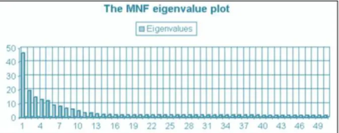
carried out by a shift difference on a specific homogenous area of the image by distinguishing adjacent pixels to each pixel and averaging the findings. The MNF transform is essentially two principal components transformations. The first transformation is based on an estimated noise covariance matrix. This first step results in transformed data in which the noise has unit variance and no band to band correlations. The second step is a standard principal components transformation. The MNF transform was carried out the AVIRIS images, resulting an output of 195 components. These components were sorted regarding to their variance. Almost 99% of total variance is presented in the 50 first components.
Figure 1. The MNF eigenvalue plot.
Figure 2 (A). MNF (1, 2 and 3) bands
Figure 3 (B). MNF (193, 194 and 195) bands 3) Excrements
In this research, pixel-based classification methods such as the spectral angle mapper, maximum likelihood classification and subpixel classification method (linear spectral unmixing) were implemented on the AVIRIS hyperspectral images. Then in order to process the mixed pixels in classification results, pixel-based and subpixel based classification algorithms were compared.
3.1) Pixel-Based Classification Methods
The probability theory to the classification task is applied by MLC method and all of the probabilities of classes for each pixel and assigning that pixel to the class with the highest probability value are computed by it. Also, the SAM considers image spectra as vectors in n-dimensional spectral space. Each spectrum defines a point in spectral space. The angle between a pair of vectors, i.e., reference spectrum and image spectrum, is a measure of the similarity of the spectra; smaller spectral angles indicate greater similarity. The differences in brightness average between spectra are important for this method, because these change the length of the spectral vector, but not its orientation. These methods was applies upon MNF images as well as on the original bands. In these procedures, 3, 5, 10, 20, 50, 87, 120, 155, 175 and 195 bands were used for classification.
3.2) Sub-Pixel Classification Method
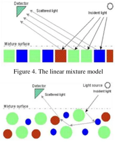
The main problem of traditional image classification procedures in classification of mixed pixel is that a single class belongs to each pixel by presuming all pixels within the image are pure. The process of mixed pixel classification tries to extract the features of the pure components of each mixed pixel. There are different models to cope with the mixed pixel problem. The nonlinear mixture model considers both the pixel of interest and the neighboring pixels i.e. each photon that reaches the sensor has interacted with multiple scattering between the different class types. The linear mixture model that assumes each pixel is modeled as a linear combination of a number of pure materials or endmembers [3]. The linear mixture model is known as
spectral unmixing. It is a method by which the user can ascertain information on a subpixel level and study decomposition of mixed pixels. The main idea of linear mixture model is that, each photon that reaches the sensor has interacted with just one class.
Figure 4. The linear mixture model
Figure 5. Non-linear mixture model
One of the limitations of non-linear spectral unmixing is that it is necessary to know the exact imaging geometry (i.e. incident and viewing angle) under which each image is captured. For accurate results one has to model the reflectivity function of each material, i.e. how much light is reflected in each direction in each wavelength. The equations relating to imaging geometry, reflectance is nonlinear. Also many surface material mix in non-linear fashions but linear unmixing method, while at best an approximation, appear to work well in many application (Boardman and Kruse, 1994). The linear mixture model which is used in this paper mixture can be mathematically described as a set of linear vector-matrix equation,
1
( . ) n
i ij j i
j
DN E F
ORDN
EF
(1)Where
i = 1, … , m (number of bands).
j = 1, … , n number of endmembers or classes). DNi is the i × 1 multi or hyperspectral vector at each
pixel.
Eij is the j × 1 endmember spectrum matrix and it is the weighting fraction of each end member. Each column in Eij matrix is the spectrum of one endmember.
Fj is the j × 1 fraction vector of each endmember for pixel.
εi is the error term of mathematical model
1 11 12 1 1 1
2 21 22 2 2 2
1 2
; ; ;
... ... ...
n n
m m m mn m m
DN E E E F
DN E E E F
DN E F
DN E E E F
the condition that all the resulting fractions must sum to unity is referred to partially constrain unmixing. However, fraction values which are negative or greater than one are still possible. Fully constrained unmixing implies an additional condition in that all determined endmember fractions must be between 0 and 1. The final results from unmixing algorithm depend on to type and number of input endmembers. Therefore, any changes applied to the reference endmembers lead to changes on the fraction map results.
In order to solve the linear unmixing problem; the sum of the coefficients should equals one, because ensure the whole pixel area is represented in the model and also each of the fraction coefficients be nonnegative to avoid negative subpixel areas. The constraint equation, can model the first requirement, for the second requirement, the coefficients need to be constrained by inequality: Fn 0 ,
1
1
Nn n
F
(2)Together, the mixing equations and the constraints describe a model that must be solved for each pixel which should be decomposed, i.e. given DN and E, we have to determine F and ε in equation (1).
4) Experiments with Pixel-Based Classification Methods
The image of Figure 6, which is a portion of the Airborne Visible/Infrared Imaging Spectrometer (AVIRIS) of hyperspectral data taken over an agricultural area of California, USA in 1994 was applied in this paper. This data has 220 spectral bands about 10 nm apart in the spectral region from 0.4 to 2.45 µm with a spatial resolution of 20 m. The image has a pixel of 145 rows by 145 columns. Figure 7. Shows the corresponding ground truth map. It includes of 12 classes.
Figure 6. RGB (31,19 and 9) MNF of image
Figure 7: The ground truth map 4.1) Maximum Likelihood Classification (MLC)
The MLC method was applied upon MNF images as well as on the original bands. This image has 220 spectral bands which 25 bands are noisy. Therefore 195 bands have been used in this research. In this procedure, 3, 5, 10, 20, 50, 87, 120, 155, 175 and 195 bands was used for classification. Table (1) shows
Overall Accuracy (OA) and Kappa coefficient (K) for this method.
Table 1. The Overall Accuracy (OA) and Kappa coefficient (K) for MLC classification
In the above Table N.B refers to the number of bands that were used for classification. Key words org, mnf refers to the original and minimum noise fraction bands, respectively.
4.2) Spectral Angle Mapper
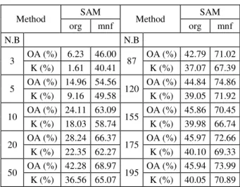
The Spectral Angle Mapper applies upon MNF images as well as original bands. In this procedure 3, 5, 10, 20, 50, 87, 120, 155, 175 and 195 bands were used for classification. Table (2) shows Overall Accuracy (OA) and Kappa coefficient (K) for this method.
Table 2. The Overall Accuracy (OA) and Kappa coefficient (K) for SAM classification
The classification accuracy can be improved by Increasing the number of bands in every two types of data. Analysis of all of the original spectral bands tends to create poor results. The classification accuracy of MNP bands are higher than the original images, because the hyperspectral image bands are often highly correlated and among them some of absorption bands contain little signal but more noise content. Using the MNF transformation on the original bands, removes the correlation between bands, separates the noise and improves the
Type of images
MLC Type of images MLC
org mnf org mnf
N.B N.B
3 OA (%) 22.98 57.93 87 OA (%) 65.89 77.92 K (%) 15.98 53.58 K (%) 61.68 75.17 5 OA (%) 31.11 61.33 120 OA (%) 79.54 81.04 K (%) 24.38 57.29 K (%) 76.84 78.62 10 OA (%) 36.29 64.88 155 OA (%) 13.83 55.41 K (%) 29.66 61.01 K (%) 00.00 51.25 20 OA (%) 54.78 69.07 175 OA (%) - 43.01 K (%) 49.73 65.51 K (%) - 38.92 50 OA (%) 59.91 73.71 195 OA (%) - 41.84 K (%) 55.21 70.52 K (%) - 37.58
Method SAM Method SAM
org mnf org mnf
N.B N.B
classification accuracy. Therefore the classification accuracy is improved. Visual and eigenvalue assessment of MNF of AVIRIS data shows that the bands numbered greater than 120 consists of data which dominated by noise. So increasing the number of bands greater than 120, decreases accuracy of the classification results. Comparing the classification results of MLC classification and SAM shows that the MLC has higher accuracy than SAM classification.
4.3) Subpixel Classification (Linear Spectral Unmixing)
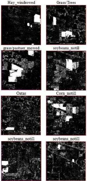
The foundation of linear unmixing is that the most of pixels are mixtures of objects. Once all the endmembers are found in an image, all the remaining pixels are considered to be linear combinations of these endmember pixels. This method was applied upon MNF images as well as original bands. In this procedure, 20, 50, 87, 120, 155, 175 and 195 number of bands were used for classification. The eight fraction images resulted of LSU have been showed in the Figure 8.
Figure 8. The fraction images of classes from the LS unmixing which is performed on the MNF bands.
Although the fraction images represent the results of subpixel classification and they do not show directly the distribution of classified areas. However, by choosing the class with the largest
pixel value in the fraction images for output, one can generate a class map that is a pixel-based representation of classification. 4.3.1) Evaluation of Linear Spectral Unmixing: After each classification its results must be evaluated and their accuracy must be assessed. According to the results type (thematic map, fraction map), an adequate strategy for accuracy assessment can be chosen. Finally to reveal the accuracy of the results, some parameters, tables and maps will be calculated and generated. Methods of accuracy assessment for traditional pixel-based classification are not fully suitable for subpixel classification. Because, our training data and ground truth are pixel-based and we couldn't find any sub-pixel based method for accuracy assessment.
There are no evaluation methods for subpixel classification and the traditional accuracy assessment procedures can’t be applied for subpixel accuracy assessment. or subpixel accuracy assessment, we have to use fraction maps as the main results of the linear unmixing classification. In the first step parameter is necessary to express the matching rate of the results with the ground truth. So we introduce the Correctness Coefficient (CC) method. Also, several procedures for subpixel accuracy assessment were introduced. A binary map from the ground truth is generated for each class to calculate of the Correctness Coefficient (CC) parameter. The numbers of binary images are equal to the number of classes or endmembers. In this research, 12 binary images are produced. The gray value of pixels in a binary image is 0 or 1. Number 1 indicates that total of this pixel belongs to the corresponding class of binary image and number 0 indicates that this pixel does not belong to corresponding class. In contrast, the results of spectral unmixing method are fraction maps in which pixel values are numbers between 0 to 1. Pixel to pixel multiplying of ground truth binary image and corresponding fraction map is an image with pixel values between zero and one.
For CC calculation, the sum of the pixel values in the above produced image is divided to the number of pixels in the land use for each fraction map. The result is a number between 0 and 1 which is named CC for linear spectral unmixing results. All pixels in land use and fraction map are the same labeled and the unmixing correctness is 100%, if CC equals 1. If CC is equal to zero then it means that no pixel in land use and fraction map has the same label and the unmixing correctness is 0%. Conceptually, this parameter is expressing the matching rate of the results of unmixing the ground truth. In this research CC calculated for each class. Total CC is calculated for linear unmixing, too. Result of this operation is shown in Table 3.
Table 3. The calculation Correctness Coefficient (CC) for linear unmixing on the MNF images
Classes Correctness Coefficient
Alfalfa 0.9641
Corn 0.8577
Corn_min 0.8211
Corn_notill 0.8596
Grass_pasture 0.7071 Grass_pasture_mov
ed
0.8546
Grass_Trees 0.9447
Hay_windrowed 0.9271
Oatas 0.9838
Soybeans_clean 0.9122 Soybeans_notill 0.8237
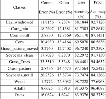
The mean of the correctness coefficients for linear unmixing is 0.8459 that indicates the result of unmixing, i.e., fraction maps are fitted with land use about 85%. This coefficient is similar to overall accuracy for pixel-based classification procedures. 4.3.2) Accuracy Assessment of Linear Spectral Unmixing Results: Accuracy assessment indices in traditional pixel-based classification methods, i.e., overall accuracy and kappa coefficient, are not suitable for subpixel classification accuracy assessment. Training data and ground truth are pixel based and we don't have any subpixel based method of accuracy assessment. In error matrix of traditional classification methods, commission error defines the percentage of those pixels that have been labeled as a particular class but in ground truth are in a different category. Omission error also defines the percentage of pixels from a particular class which have been labeled as the other classes. So omission and commission errors for each class can be calculated by using subpixel classification results. For this purpose, first the ground truth of the image converted to binary images. The numbers of binary images and the number of classes or endmembers are the same. In this research, 12 binary images are produced. The gray value of pixels in a binary image is 0 or 1. In contrast, the results of spectral unmixing method are fraction maps in which pixel values are numbers among 0 to 1. Pixel to pixel differencing of ground truth binary image and corresponding fraction map is an image in which the pixel values are negative, zero or positive. A zero pixel value indicates that this pixel was correctly classified, i.e., 100%. Negative pixel value indicates the incorrectly classified percent of that pixel and belongs to other classes in the ground truth. This error is equivalent with the commission error in the traditional pixel-based classification. Similarly, positive pixel values indicates the percent of pixel that does not classified correctly but in ground truth belongs to this class. This error is equivalent with omission error in traditional pixel-based classification. The Table (4) shows result of the calculation.
Classes
Comm Error (%)
Omm Error (%)
User Accuracy
(%)
Prod Accuracy
(%) Hay_windrowed 11.3354 7.2874 88.6646 92.7126
Corn_min 34.9005 12.7987 65.0995 87.2013 Corn_notill 10.6819 15.6105 89.3181 84.3895 Corn 32.9771 19.6302 67.0229 80.3698 Grass_pasture_moved 20.0045 17.7140 79.9955 82.2860 Soybeans_clean 41.1789 9.7694 58.8211 90.2306 Grass_Trees 33.5519 5.5348 66.4481 94.4652 Grass_pasture 11.2371 23.1949 88.7629 76.8051 Soybeans_notill 35.1226 22.7795 64.8774 77.2205 Wood 9.9695 3.7110 90.0305 96.2890 Alfalfa 9.9695 3.7110 90.0305 96.2890 Oatas 16.0624 1.6241 83.9376 98.3759 Table 4. Estimation of error in linear spectral unmixing for
original images (120 bands)
According to the findings of original images, the average producers accuracy is 88.05% and user’s accuracy is 77.75% for classes. These accuracy parameters on the MNF images are shown in Table (5).
Classes
Comm Error (%)
Omm Error (%)
User Accuracy
(%)
Prod Accuracy
(%) Hay_windrowed 11.8156 7.2874 88.1844 92.7126
Corn_min 18.2697 12.1381 81.7303 87.8619 Corn_notill 3.8830 12.8569 96.1170 87.1431 Corn 30.4930 13.4164 69.5070 86.5836 Grass_pasture_moved 3.2760 12.7402 96.7240 87.2598 Soybeans_clean 17.7028 8.2870 82.2972 91.7130 Grass_Trees 33.5519 5.5348 66.4481 94.4652 Grass_pasture 2.8436 24.4573 97.1564 75.5427 Soybeans_notill 26.2526 15.8734 73.7474 84.1266 Wood 1.2772 22.3032 98.7228 77.6968 Alfalfa 8.6625 3.5913 91.3375 96.4087 Oatas 16.0624 1.6241 83.9376 98.3759 Table 5. Estimation of error in linear spectral unmixing method
for MNF images (120 bands)
Based in the results on the MNF images, it can be said that the average producers accuracy is 88.32% and user’s accuracy is 85.49% for classes (see Table 5). It is clear, that applying MNF on the original images, users and producers accuracy is improved. The overall accuracy can be used to summarize the classification results. Table (6) shows the OA estimation for linear spectral unmixing classification results.
Table 6. Estimation of overall accuracy (OA) for LSU classification (120 bands)
5) Comparison between Accuracy of Sub-Pixel and Pixel-Based Classification
This comparison was implemented between users and producers accuracy as well as overall accuracy of Subpixel and Pixel-Based Classification method for evolution of the decomposing of mixed pixel. Table (7) shows users and producer’s accuracy for original images in the three classification method.
Type of images
On diag pixel on The Original
images (N)
On diag pixel on The Mnf images (N)
Num pixel on the Ground
truth (N) Hay_windrowed 453.3647 453.3647 489
Corn_min 679.2588 684.7680 834
Corn_notill 1194.100 1232.600 1434
Corn 488.4706 526.6235 614
Grass_pasture_moved 2010.200 2131.300 2494 Soybeans_clean 551.0157 560.1176 614
Grass_Trees 661.7922 705.6549 747 Grass_pasture 357.7216 351.4471 497 Soybeans_notill 1194.100 1232.600 968
Wood 968.0510 986.3961 1294
Alfalfa 91.4745 91.5882 95
Method
Org_Unmix Org_MLC Org_SAM P.Acc
(%) U.Acc
(%) P.Acc
(%) U.Acc
(%) P.Acc
(%) U.Acc
(%) classes
Hay_windrowed 92.72 88.67 92.84 76.82 99.39 55.48 Corn_min 87.20 65.09 55.76 33.03 50.48 24.52 Corn_notill 84.39 89.32 51.19 60.81 24.62 32.24 Corn 80.37 67.02 34.87 41.36 14.43 24.7 Grass_pasture_
moved
82.29 79.99 39.55 72.3 20.95 76.37 Soybeans_clean 90.24 58.82 55.54 34.1 45.77 24.65 Grass_Trees 94.47 66.45 77.11 79.89 48.19 71.43 Grass_pasture 76.81 88.77 64.19 62.92 3.02 4.18 Soybeans_notill 77.23 64.88 54.03 39.71 70.25 43.15
Wood 76.13 88.69 76.43 62.24 88.1 74.85 Alfalfa 96.29 90.04 96.84 36.65 100 39.09 Oatas 98.38 83.94 96.23 64.15 93.4 82.85 Table 7. The comparison users and producer’s accuracy for
original images (120 bands)
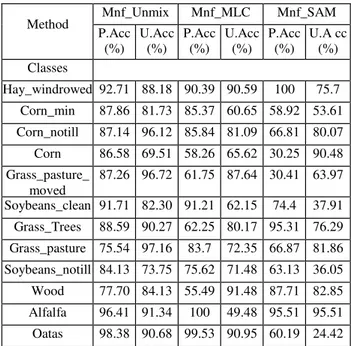
Also, the users and producer’s accuracy for MNF images in the three classification method are shown in Table (8).
Method Mnf_Unmix Mnf_MLC Mnf_SAM
P.Acc (%)
U.Acc (%)
P.Acc (%)
U.Acc (%)
P.Acc (%)
U.A cc (%) Classes
Hay_windrowed 92.71 88.18 90.39 90.59 100 75.7 Corn_min 87.86 81.73 85.37 60.65 58.92 53.61 Corn_notill 87.14 96.12 85.84 81.09 66.81 80.07 Corn 86.58 69.51 58.26 65.62 30.25 90.48 Grass_pasture_
moved
87.26 96.72 61.75 87.64 30.41 63.97 Soybeans_clean 91.71 82.30 91.21 62.15 74.4 37.91 Grass_Trees 88.59 90.27 62.25 80.17 95.31 76.29 Grass_pasture 75.54 97.16 83.7 72.35 66.87 81.86 Soybeans_notill 84.13 73.75 75.62 71.48 63.13 36.05 Wood 77.70 84.13 55.49 91.48 87.71 82.85 Alfalfa 96.41 91.34 100 49.48 95.51 95.51 Oatas 98.38 90.68 99.53 90.95 60.19 24.42 Table 8. The comparison users and producers accuracy for MNF
images (120 bands)
Table (8) shows the results of classification by overall accuracy parameter for pixel-based, SAM and MLC, and subpixel based (LSU) methods. Finally, comparison of overall accuracy is applied between the three classification methods. Table (9) shows this comparison.
Method LSU MLC SAM
Image Original MNF Original MNF Original MNF Over.
Accuracy
(%)
86.07 89.05 79.54 81.04 44.84 74.86
Table 9. The Comparison of overall accuracy (OA) (120 bands) As can be seen form above Tables, the minimum difference the between pixels based accuracy and subpixel based accuracy which was performed on the MNF images are 8% and 12%, respectively because pixel-based methods has high accuracy in 120 bands. It is clear that LSU is a robust procedure for hyperspectral images classification.
6) Conclusion
It can be concluded that: In all of the classification algorithms were used in this research, increasing the number of bands, makes increasing the classification accuracy consequently. Therefore, by development of remote sensing technology and using of the new sensors with hyperspectral capabilities in RS science, it is better to use these images in classification process. In pixel based classification approaches such as maximum likelihood classification and Spectral angle mapper, increasing the number of bands (above 120), decreases the accuracy of classification results. Therefore using new image processing tools and techniques are introduced for hyperspectral images classification is offered. By applying Minimum Noise Fraction (MNF) transformation on the hyperspectral images, the correlation and noises from bands can be removed and we can sort them according to their variance. In the bands with a high variance, the features can distinguish from each other in a better mode, therefore classification accuracy increased sensibly. Using MNF transformation on images which used for classification, the individual class’s accuracy is increased about 15 to 20 percent from pixel based procedures and 9 percent from unmixing method, when applying on source image. Applying MNF transformation on the hyperspectral images reduces the dimensionality of hyperspectral image data for next processing. In pixel-based classification approaches such as maximum likelihood classification and spectral angle mapper, increasing the number of bands (more than 120)we have a decrease in accuracy of the classification results. But in linear unmixing method there is no limitation in the number of bands and by increasing the number of bands the remaining amount of spectral decomposition for each pixel is minimized i.e., accuracy of subpixel classification is increased. Table (10) shows that increasing the number of bands; decreasing the RMS error of each pixel in model. This decreasing of RMS error is obviously seen in both of the original and MNF images.
Type of Images LSU
org mnf
N.B
20 RMS Mean Error 1.992245 0.118545 50 RMS Mean Error 2.647923 0.128302 87 RMS Mean Error 2.45367 0.128193 120 RMS Mean Error 2.340894 0.126726 155 RMS Mean Error 2.133099 0.124806 175 RMS Mean Error 2.031512 0.123393 195 RMS Mean Error 1.938037 0.122026
Average RMS Mean Error
2.219626 0.12457
Table 10. RMS Error Mean unmixing
producers’ accuracy for original images, users and producers’ accuracy for MNF images and overall accuracy. Average of the comparison parameters is shown in the Table (11).
Method LSU MLC SAM
Type of
images Original MNF Original MNF Original MNF User.
Accuracy (%)
86.38 87.83 66.21 79.18 54.88 69.13
Prod. Accuracy (%)
77.64 86.82 55.33 75.30 46.13 66.56
Over. Accuracy (%)
86.07 89.05 79.54 81.04 44.84 74.86
Comparison
Methods SAM and LSU MLC and LSU
Type of images
Original MNF Original MNF Min.Diff.
User. A (%)
31.45 18.70 20.17 8.65
Min.Diff.Prod .A(%)
31.51 20.26 22.31 11.52
Min. Diff. OA (%)
41.23 14.19 6.53 8.01
Table 11. The comparison of average accuracy for pixel based and subpixel classification (120 bands)
The table above reveals that, the spectral unmixing method that implemented here is an effective technique for classifying a hyperspectral image. Classification results by applies on the original images are not appropriate because some of the hyperspectral image bands are subject to absorption and they contain only little signal but more noise content. Also, applying the minimum noise fraction transformation on the hyperspectral images increased the individual classes accuracy of pixel based classification methods as well as unmixing method about 15 to 20 percent and 8 percent respectively. Therefore, linear spectral unmixing is in the beginning of its growth and will be found many applications in many of branch science in the future.
7) References
[1] Abkar A.A. (1999). “Likelihood-Based Segmentation and Classification of Remotely
Sensed”. ITC publication number 73.
[2] Proffesor Maria Petrou “Tutorial on modern techniques in remote sensing”, School of
Electronic Engineering, Information Technology and Mathematics, University of Surrey, Gui
ldford,
http\\www.survey.ntua.gr/main/Labs/ rsens/DeCETI/ [3] P. Gong, J.R. Miller, J. Freemantle, and B. Chen. (1991). “Spectral decomposition of Landsat
Thematic Mapper data for urban land-cover mapping”, Calgary, Alberta, Canada.
[4] Dr. Robert A. Schowengerdt, (2000).,“Subpixel Classification”. http//:www.arizona.edu.
[5] J.J. Settle and N.A. Drake, (1993), "Linear mixing and the estimation of ground cover
proportions". International Journal of Remote Sensing. [6] D. Heinz, C-I. Chang, M.L.G. Althouse,( 1999). "Fully constrained least-squares based linear