A modified interactive procedure to solve multi-objective group decision making problem

(1)

* Corresponding Author. Email address: m_izadikhah@yahoo.com, m-izadikhah@iau-arak.ac.ir

A modified

interactive procedure to solve

multi-objective group

decision making problem

Mohammad Izadikhah*

Department of Mathematics, College of Science, Arak-Branch, Islamic Azad University, Arak, Iran.

Copyright 2014 © Mohammad Izadikhah. This is an open access article distributed under the Creative Commons Attribution License, which permits unrestricted use, distribution, and reproduction in any medium, provided the original work is properly cited.

Abstract

Multi-objective optimization and multiple criteria decision making problems are the process of designing the best alternative by considering the incommensurable and conflicting objectives simultaneously. One of the first interactive procedures to solve multiple criteria decision making problems is STEM method. In this paper we propose a modified interactive procedure based on STEM method by calculating the weight vector of objectives which emphasize that more important objectives be closer to ideal one. We use the AHP and TOPSIS method to find these weights and develop a multi-objective group decision making procedure. Therefore the presented method tries to increase the rate of satisfactoriness of the obtained solution. Finally, a numerical example for illustration of the new method is given to clarify the main results developed in this paper.

Keywords: AHP; TOPSIS; MCDM; MODM; MADM; MOLP; STEM.

1 Introduction

Multi-objective optimization (or objective programming), also known as criteria or multi-attribute

optimization, is the process of simultaneously optimizing two or more conflicting objectives subject to certain constraints. Multi-objective optimization problems can be found in various fields: product and process design, finance, aircraft design, the oil and gas industry, automobile design, or wherever optimal decisions need to be taken in the presence of trade-offs between two or more conflicting objectives. Maximizing profit and minimizing the cost of a product; maximizing performance and minimizing fuel consumption of a vehicle; and minimizing weight while maximizing the strength of a particular component are examples of multi-objective optimization problems.

Optimization can be used only when there is a single objective. The feasible solutions can then be ranked unambiguously according to this objective and the optimal one identified. In the real-world, almost every important problem involves more than one objective. When there is more than one objective, and the objectives are non-commensurate, which means they cannot be transformed into a single objective, the

Available online at www.ispacs.com/dea Volume: 2014, Year 2014 Article ID: dea-00068, 23 Pages

doi:10.5899/2014/dea-00068

(2)

International Scientific Publications and Consulting Services

"optimal" no longer has the same "objective" sense as before. A compromise solution must now be selected on the basis of the decision maker's attitude to achievement of the various objectives. For nontrivial multi-objective problems, one cannot identify a single solution that simultaneously optimizes each objective. While searching for solutions, one reaches points such that, when attempting to improve an objective further, other objectives suffer as a result. A tentative solution is called non-dominated, Pareto optimal, or Pareto efficient if it cannot be eliminated from consideration by replacing it with another solution which improves an objective without worsening another one. Finding such non-dominated solutions, and quantifying the trade-offs in satisfying the different objectives, is the goal when setting up and solving a multi-objective optimization problem.

There are several approaches to obtaining such solutions. Based on the ways of extracting the decision maker's preference information and using it in decision analysis processes, the MODM methods can be divided into three main categories (Hwang et al., 1979) [15]:

 Priori articulation of preference information.

The most common way of conducting MODM is by priori articulation of the DM's preferences. This means that before the actual optimization is conducted, the different objectives are somehow aggregated to one single figure of merit. Weighted sum (Steuer, 1986) [30], non-linear combination (Andersson, 1998 [2]; Krus et al., 1995) [21], utility theory (Keeney et al., 1976) [19], fuzzy logic (Chiampi et al., (1996,1998) [11, 10]; Zimmermann et al., 1995 [35]), acceptability functions (Kim et al., 1997 [20]; Wallace et al., 1996 [32]), and goal programming (Tamiz et al., 1998 [31]; Steuer, 1986 [30]; Charnes et al., 1955, 1961 [8, 7]) methods belong to this category. An obvious drawback of this category is that, in the case of a large number of objective functions, the appropriate weighting is difficult to choose.

 Progressive articulation of preference information.

The methods of this category are generally referred to as interactive ones. They rely on progressive information about the DM`s preferences simultaneously as they search through the solution space. Typically, the optimization program provides an updated set of solutions and lets the DM consider whether or not the weighting of individual objective functions. Tchebychev method (Steuer, 1986) [30], and STEM method ( Benayoun et al., 1971) [6], are most common in this category. These methods do not need "a priori" preference information. The DM could give some preference information as the search moves on. Therefore, it is a learning process where the DM gets a better understanding of the problem. However, the solutions are dependent upon how well the DM can articulate his or her preferences and how much effort is required from the DM during the entire search process. In addition, if the preferences are changed, the process has to be restarted. Jeong and Kim (2005) [17], proposed a modified STEM, called D-STEM, to overcome the methodological limitations of STEM. D-STEM utilized the concept of a desirability function to realistically model the differing degrees of satisfaction. D-STEM also allowed a DM to choose either tightening or relaxation, which makes the preference articulation process more efficient and effective.

 Posteriori articulation of preference information

A number of algorithms can generate a set of Pareto optimal solutions and present them to the DM. The e-constraint method (Crossley et al., 1999) [12], normal boundary interaction (Das, 1998) [13], and Generate First-Choose Later (GFCL)

approach (Balling and Richard, 1999 [4]; Balling, 2000 [3]; Hwang and Masud, 1979 [15]) belong to this category.

As discussed above, each MODM method has pros and cons. Generally, none of them is superior to the others.

(3)

makers and the weights of objectives and therefore we determine the importance of the objectives and consider this importance into decision making process.

The Technique for Order Preference by Similarity to an Ideal Solution (TOPSIS) method is presented in Chen and Hwang (1992) [9], with reference to Hwang and Yoon, (1981) [16]. The basic principle is that the chosen alternative should have the shortest distance from the ideal solution and the farthest distance from the negative ideal solution. Yue, (2011) [33], developed an extended TOPSIS for determining weights of decision makers with interval numbers. Also, Yue, (2011) [34], proposed a new approach for determining weights of DMs in group decision environment based on an extended TOPSIS method. Decision making nowadays assumes scientifically supported process, which in most cases includes several decision makers and interest groups. To successfully deal with different attitudes and opinions of different people, variety of methods is in use. Not many of them can involve quantitative, qualitative and semi-qualitative criteria as the Analytic Hierarchy Process (AHP) can do; and this is probably the main reason why it is popular worldwide.

The major advantage of AHP is that it involves a variety of tangible and intangible goals. For instance, it reduces complex decisions to a series of pair-wise comparisons, implements a structured, repeatable and justifiable decision making approach and build consensus (Srdjevic et al, 2007) [29]. An introduction to the method and its theoretical foundations is given in Saaty (1980) [26]; for this reason only the basic properties of the method that are necessary for understanding the decision-making process will be described in the next section. There is a visible abundance literature on the refinements and generalizations of AHP model as well as various applied studies (see for example, Dong et al., 2010, 2011) [14].

The obtained weights of objectives in the proposed method is such that they emphasize that more important objectives be more closer to ideal one. STEM or Step Method proposed by Benayoun, de Montgolifer, Tergny and Laritchev (1971) [6], is a reduced feasible region method for solving the MOLP

1

max { ( ),..., ( )}

. .

k

f x f x s t

xS (1.1)

Where all objectives are bounded over S. Each iteration STEM makes a single probe of the efficient set. This is done by computing the point in the iteration's reduced feasible region whose criterion vector is closest to ideal criterion vector. STEM is one first interactive procedure to have impact on the field of multiple objective programming.

Therefore the presented method try to increase the rate of satisfactoriness of the obtained solution. Rest of the paper is organized as follows:

In section 2, some preliminaries about the concepts of MODM problems, STEM method, AHP, TOPSIS and related topics are given. In section 3, we will propose a method for determining weights of DMs by TOPSIS method. In section 4, we will focus on the proposed method. In section 5, a numerical example is demonstrated. And finally in section 6, some conclusions are drawn for the study.

2 Preliminaries

In this section we express the following useful concepts that are given from Lu et al. (2007) [23].

2.1. MODM Problems

(4)

some of them conflict. In the other words, decisions in the real world contexts are often made in the presence of multiple,

conflicting, and incommensurate criteria.

Multi-criteria decision making (MCDM) refers to making decision in the presence of multiple and conflicting criteria. Problems for MCDM may range from our daily life, such as the purchase of a car, to those affecting entire nations, as in the judicious use of money for the preservation of national security. However, even with the diversity, all the MCDM problems share the following common characteristics:

 Multiple criteria: each problem has multiple criteria, which can be objectives or attributes.  Conflicting among criteria: multiple criteria conflict with each other.

 Incommensurable unit: criteria may have different units of measurement.

 Design/selection: solutions to an MCDM problem are either to design the best alternative(s) or to select the best one among previously specified finite alternatives.

There are two types of criteria: objectives and attributes. Therefore, the MCDM problems can be broadly classified into two categories:

 Multi-objective decision making (MODM)  Multi-attribute decision making (MADM)

The main difference between MODM and MADM is that the former concentrates on continuous decision spaces, primarily on mathematical programming with several objective functions, the latter focuses on problems with discrete decision spaces.

Multi-objective decision making is known as the continuous type of the MCDM. The main characteristics of MODM problems are that decision makers need to achieve multiple objectives while these multiple objectives are non-commensurable and conflict with each other. An MODM model considers a vector of decision variables, objective functions, and constrains. Decision makers attempt to maximize (or minimize) the objective functions. Since this problem has rarely a unique solution, decision makers are expected to choose a solution from among the set of efficient solutions (as alternatives). Generally, the MODM problem can be formulated as follows:

max ( )

) . .

f x

MODM s t

x S

   

 _

 (2.2)

where represents n conflicting objective functions, and is an -vector of decision variables,

.

n

x



R

Example 2.1. (Example of MODM problem)

For a profit-making company, in addition to earning money, it also wants to develop new products, provide job security to its employees, and serve the community. Managers want to satisfy the shareholders and, at the same time, enjoy high salaries and expense accounts; employees want to increase their take-home pay and benefits. When a decision is to be made, say, about an investment project, some of these goals complement each other while others conflict.

2.2. Basic Definitions

(5)

Definition 2.1.

x

*is said to be a complete optimal solution, if and only if there exists an

x

*



X

such that *

( ) ( ), 1,..., ,

i i

f x  f x i k for all xX .

Also, ideal solution, superior solution, or utopia point are equivalent terms indicating a complete optimal solution.

In general, such a complete optimal solution that simultaneously maximizes (or minimizes) all objective functions does not always exist when the objective functions conflict with each other. Thus, a concept of Pareto-optimal solution is introduced into MOLP.

Definition 2.2.

x

*is said to be a Pareto optimal solution, if and only if there does not exist another *

x



X

such that f x_i( ) f x_i( )* for all

i

and

f x

_j

( )



f x

_j

( )

* for at least one

j

.

Also, ideal solution, superior solution, or utopia point are equivalent terms indicating a complete optimal solution.

The Pareto optimal solution is also named differently by different disciplines:

non-dominated solution, non-inferior solution, efficient solution, and non-dominate solution.

Definition 2.3. (Satisfactory Solution) A satisfactory solution is a reduced subset of the feasible set that exceeds all of the aspiration levels of each attribute. A set of satisfactory solutions is composed of acceptable alternatives. Satisfactory solutions do not need to be non-dominated.

Definition 2.4. (Preferred Solution) A preferred solution is a non-dominated solution selected as the final choice through decision maker's involvement in the information processing.

In the presented method (and in traditional STEM method), in order to measure the distance between two vectors we use the following metric:

Definition 2.5. Consider the weight vector



where

1

k i i







and



_i



0

. These weights define the weighted Tchebychev metric:





* *

1,...,

( ) max _i _i _i( )

i k

f f x 



f f x  

   (2.3)

2.3. STEM Method

(6)









1

* 1

1

min ( )

. .

1,

0.

p

k _h p

i i i i

h k _h

i i h i

w f f x

s t

x S w w





  



(2.4)

is the iteration counter, and p is the parameter in the L_p-norm, usually equaling 1 or 2. The weights are needed in order to solve the min-max formulation and to equalize the magnitude of the different objectives. The weights are not crucial to the outcome of the optimization as the final solution is obtained by means of bounds on the objective rather than variation of weightings. In the literature methods of calculating the weights are given. The problem is solved resulting in an objective vector f . f is compared with the ideal solution

F

*. If some components of f are acceptable but some are not, the decision-maker must decide on a relaxation on at least one of the objectives. This means that the upper bound for the -th objective are adjusted to

f

_j

 

f

_j. The solution space

S

h1is reduced by the new constraint

f

_j



f

_j

 

f

_j. The weighting of the -th objective is set to zero and the optimization problem of is solved again, this time in the reduced solution space.

After the second iteration, the decision-maker might be satisfied with the obtained solution, or he/she has to relax the boundaries of another function and start over again. Thus, the algorithm proceeds through progressively reducing the solution space by introducing new constraints on the different objectives.

2.4. AHP method

Given a finite number of alternatives, say various options, solutions, etc.

a

1

,...,

a

n, etc. to be considered in

a certain investment scenario, the objective is to order them by associating with them some degrees of preference expressed in the [0,1] interval. The essence of the method introduced by Saaty is to determine such preference values through running a series of pairwise comparisons of the alternatives and called AHP.

The AHP is widely used as one of the major MADM methods for solving a wide variety of problems that involve complex criteria across different levels in which the interaction of criteria is common (Saaty, 1977, 1980) [25, 26]. The AHP is a powerful and flexible decision making process to help people set priorities and make the best decision when both the qualitative and quantitative aspects of a decision need to be considered (Malik and Sumaoy, 2003). It breaks down a complex multicriteria decision problem into smaller constituents and forms a multi-level hierarchical structure. An AHP generally consists of following steps: (Lee et al., 2007) [22]:

1. The AHP is a multi-criteria decision-making method which requires a well-structured problem, represented as a hierarchy. Usually, at the top of the hierarchy is the goal; the next level contains the criteria and sub-criteria, while alternatives lie at the bottom of the hierarchy.

(7)

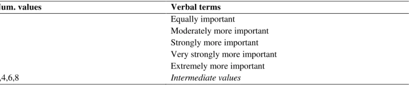
Table 1: The fundamental Saaty’s scale for the comparative judgments

Num. values Verbal terms

1 Equally important

3 Moderately more important

5 Strongly more important

7 Very strongly more important

9 Extremely more important

2,4,6,8 Intermediate values

By assumption, value 1 corresponds to the case in which two elements contribute in the same way to the element in the higher level. Value 9 corresponds to the case in which one of the two elements is significantly extremely more important than the other. Also, if the judgment is that B is more important than A, the reciprocal of the relevant index value is assigned. For example, if B is felt to be notably Very strongly more important as a criterion for the decision than A, then the value

1

7

would be assigned to A

relative to B. The results of the comparison are placed in comparison matrices. It is important to note that the efficiency of an AHP greatly depends on the accuracy of the pairwise weights. If there are attributes in a level, then the squared matrix of attributes with respect to a higher attribute or goal will be presented as (2.5).

 

11 12 1

21 22 2

1 2

n n ij

n n nn

a a a

A a

a a a

 

 

 

 

 

(2.5)

where a_ijdenotes the importance of -th attribute with respect to -th attribute. Also, it is assumed that

1

ji ij

a



.

3. In this stage, the weights to be assigned to the decision- making attributes are calculated via eigenvectors. The eigenvector calculation is widely used to determine the relative weights of attributes from the results of pairwise comparison. Briefly, in this approach, the eigenvalue from the comparison matrix is calculated and then the eigenvector that corresponds to the maximum eigenvalue is determined via (2.6) to normalize the weights so that their sumequals1 (Saaty,1980) [26].

To indicate whether the ordinal ranking of the pairwise comparisons obtained from expert evaluations are reliable, a measure called the consistency ratio (CR) is defined. If this measure is less than , the results are acceptable.

max

(

A





I w

)



0

(2.6)

where



_maxis the maximum eigenvalue and is its corresponding eigenvector, see Agalgaonkar et al., (2006) [1].

(8)

dimensionality of the reciprocal matrix (recall that in reciprocal matrices the elements positioned symmetrically along the main diagonal are inverse of each other),



_max



n

where the equality



_max



n

occurs only if the results are fully consistent. The ratio

max

(

)

(

1)

n

v

n









(2.7)

can be regarded as a certain consistency index of the data; the higher its value, the less consistent are the collected experimental results. This expression can be sought as the indicator of the quality of the pairwise assessments provided by the expert. If the value of certain superimposed threshold, the experiment may need to be

the assessment is sought to -examination of the

experimental data and a re-run of the experiment. The threshold of the consistency ratio expressed as the ratio of the consistency index, and the random consistency index , _CR CI

RI

 is also established (typically assuming the value of 0.1) to assess the quality of the results of pairwise comparison, (see Belton, 1986) [5].

2.5. TOPSIS Method

TOPSIS (technique for order preference by similarity to an ideal solution) method is presented in Chen and Hwang with reference to Hwang and Yoon. TOPSIS is a multiple criteria method to identify solutions from a finite set of alternatives. The basic principle is that the chosen alternative should have the shortest distance from the positive ideal solution and the farthest distance from the negative ideal solution.

2.6. Aggregation of Individual Judgments

In order to aggregate all the individual Judgments and construct one group Judgments we need to construct aggregated pair-wised comparison matrix. Assume that we have decision makers (we denoted by

D

t,

1,...,

t



k

). Let

A

t,

t



1,...,

k

be the pair-wised comparison matrices that

A

t shows the pair-wised comparison matrix for evaluating n criteria made by

D

t. Let the pair-wise comparison (judgment) matrix

for the

D

tbe given by

 

t t

ij _{n n}

A

a





and let



t

,

t



1,...,

k

be the corresponding importance of the -th

decision maker in contributing to the group judgment. Then, we can obtain a group judgment matrix (group pair-wised comparison matrix)

 

_ij

n n

A

a





by using following formula

 

1

k t ij _{n n} t

t

A a



A

 

 



_(2.8)

Therefore we have

1

k t ij t ij

t

a



a





.

3 Determining weights of DMs by TOPSIS method

(9)

individual decision matrix. In this paper we obtain the DM’s weights from the pair-wised comparison matrices by defining the ideal pair-wised comparison matrix as follows:

Let t

 

t ij _{n n}

A a



 be the pair-wised comparison matrix of th DM. As described in Yue, in mean sense, the best result of group decision making should be the average pair-wised comparison matrix of group decision:

 

11 12 1

21 22 2

1 2

n n ij

n n nn

a a a

A a

a a a

                  _ _       (3.9) Where 1

1

k _t

t

A

k







and

1

k _t

ij _t ij

a

k







. We call

A

 as the ideal pair-wised comparison matrix. In order to determine the weights of decision makers, we use the following concept:

The less the distance of judgment of

D

_t from the ideal judgment the higher importance for

D

_tis expected.

In other words, a DM is higher decision level because his/her opinion is closer to average (ideal). So we define

A

 as the Positive ideal solution. For the pair-wised comparison matrix

A

tof th DM, the closer the ideal matrix

A

, the more the weight of th DM.

In order to measure decision level of each DM, we can calculate the distance between each individual pair-wised comparison matrix

A

t and the ideal pair-wised comparison matrix

A

. Consider that the Euclidean distance is the most widely used tool to measure the separation of two objects in practical applications, we utilize it to measure the separation between

A

tand

A

. The separation of each individual decision

A

tform the

A

, is given as:





1 2 2 1 1 n n t t

t ij ij

i j

d



A



a



 











_



_







(3.10)

In this sense, the smaller distanced_t, the better judgment

A

tof th DM. Considering that, in mean sense, for a DM, the maximum risk is the maximum separation from the average matrix of group judgment. And the average matrix of group judgment is the distributing center of all matrixes of group judgment, for this reason, we define following left and right maximum separation from the average matrix of group judgment. That is, we divide the negative ideal solutions (NISs) into two parts: L-NIS

A

l and R-NIS

A

r, respectively, as follows:

 

11 12 1

21 22 2

1 2

l l l

n

l l l

l l n

ij

l l l

n n nn

a a a

A a

a a a

(10)

 

11 12 1

21 22 2

1 2

r r r

n

r r r

r r n

ij

r r r

n n nn

a a a

A a

a a a

       _ _       (3.12) where 1

min {

|

}

l t t

ij ij ij ij t k

a



 





and

1

max {

|

}

r t t

ij ij ij ij t k

a



 





. In fact,

a

ijl and r ij

a

are the minimum and maximum matrices of group decision, respectively.

Similarly, the separations of each individual decision form the NISs, dtl



and dtr



, are given respectively as





1 2 2 1 1 n n

l t l t l

t ij ij

i j

d



A

a

 











_



_







(3.13) And





1 2 2 1 1 n n

r t r t r

t ij ij

i j

d



A

a

 











_



_







(3.14)

Clearly, the larger the separations d_tl and d_tr, the better the judgment

A

tof -th DM. Therefore, similar to (3.10), a closeness coefficient is defined to determine the ranking order of all DMs once the d_tl and

r t

d have been calculated. The closeness coefficient of the -th DM with respect to

A

is defined as:

l r t t

t l r

t t t

d

R

d

    







(3.15)

Clearly,

R

_t



[0,1]

.

Obviously, an individual pair-wised comparison matrix

A

t is closer to the

A

and farther from

A

l as well as

A

r, and as

R

_tapproaches to 1. Then, we can determine the weights of decision makers according to the above similarity measure.

Assume that the weight of

D

t is denoted by



t. Hence, we can determine each



t

,

t



1,...,

k

as follows:

1 t t k t t

R







(3.16)

The above weights are such that

1

1,

0.

k

t t

t











4 Improved STEM method

The procedure for improving STEM method has been given as following steps:

Step 0. Preparing the problem

(11)

1

max { ( ),..., ( )}

. .

k

f x f x s t

xS (4.17)

The method requires that the DM gives a vector of weight relating the objectives. Assume that there are decision makers,

D

₁

,...,

D

_k. In order to determine the importance of objectives, each decision maker gives a pair-wised comparison matrix. Let the pair-wise comparison (judgment) matrix for the

D

tbe given

by t

 

t ij _{n n}

A a



 as follows:

 

11 12 1

21 22 2

1 2

t t t

n

t t t

t t n

ij

t t t

n n nn

a a a

A a

a a a

 

 

 

 

 

(4.18)

Step 1. Determining weights of DMs

By using the above mentioned procedure, we can determine the weights of decision makers. Consider the obtained weight of decision maker -th,

D

t, be



t.

Step 2. Aggregating of Individual Judgments

By a method discussed above, we aggregate all Individual Judgments and obtain one pair-wised comparison matrix as

A



 

a

ij _{n n}_ where

1

k t ij t ij

t

a



a





Step 3. Calculating the weight vector of objectives.

As discussed above, the method requires that the DM gives a vector of weight relating the objectives. This weight is calculated by the AHP method that mentioned above. is generally normalized so that

1

k i i

W





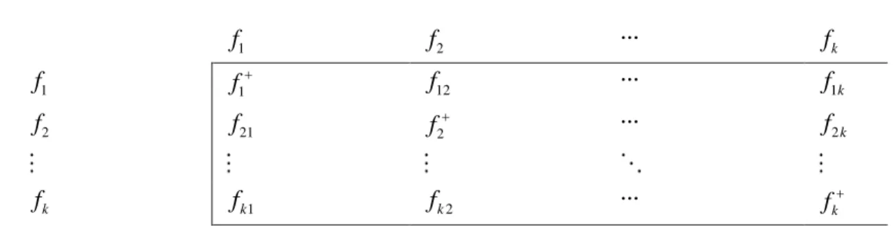
and the bigger weighting coefficient is associated with the more important objectives.

Step 4. Construct the pay-off table.

In this step we first maximize each objective function and construct a pay-off table to obtain the ideal criterion vector

f





R

k.

Let

f

_j

,

j



1,..., ,

k

be the solutions of the following problems, namely, the ideal solution:

max ( )

. .

j j

f f x

s t

x S  _

 (4.19)

(12)

Table 2: Pay-off table

1

f

₂

...

f

_k

1

f

f₁

f

₁₂

...

f

₁_k

2

f

₂₁ f₂

...

f

2k

k

f

_k₁

f

_k₂

...

f_k

In Table 2, row corresponds to the solution vector

x

j which maximizes the objective function f_j. A f_ij

is the value taken by the th objective

f

_jwhen the -th objective function f_i reaches its maximum f_i, that is,

f

_ij



f x

_j

(

i

)

. Then the positive ideal criterion can be defined as follows:



 

1



1 ,..., 1( ),..., ( )

k

k k

f  f f  f x f x  (4.20)

And consider that

x

be the inverse image of

f

. Generally, we know it is may be

x

not belong to

S

( )h .

Step 5. Calculate the weight factors.

Let f_iminbe the minimum value in the -th column of the first pay-off table (Table 2). Calculate



i values where:

1 min 2 2 1 1 min 2 2 min 1

,

0,

,

0,

n i i ij i j i i n i i ij i j i

f

c

f

c

f



        



_

_





_

_

_













 



_

_

_



_

_

_







_

_





(4.21)

Where c_ijare the coefficients of the -th objective. Then, the weighting factors can be calculated as follows:

1

, 1,...,

i i k j j i k







  



(4.22)

The weighting factors defined as above are normalized, that is they satisfy the following conditions:

0  



_i

1,

i



1,...,

k

and

1

k i i







(4.23)

(13)

Step 6. Calculation Phase.

The weight factors defined by formula (4.22) are used to apply the weighted Tchebychev metric, Def. 5, to obtain a compromise solution, also, the weight vector of objectives are used to emphasize that more important objectives be closer to ideal one.

We can obtain a criterion vector which is closest to positive ideal one and emphasize that more important objectives be more closer to ideal one by solve the following model:

( )

min

. .

(

( ))

0

h

s t

W f

f x

x

S

R









_

_



 

(4.24)

This model can be converted to the following model:

( )

min

. .

( ( )) , 1

0

i i i i h

s t

W f f x i k

x S R







_ _ _{ }

  

(4.25)

We solve the weighted minimax model (4.25) and obtain the solution

x

( )h . By solving the model (4.25) we obtain a compromise solution as

x

( )h . In the other words, we obtain a compromise solution

x

( )h in the reduced feasible region

S

( )h whose criterion vector is closest to positive ideal criterion vector

f

.

Step 7. (Decision phase)

The compromise solution

x

( )h is presented to the decision maker, who compares objective vector

(

( )h

)

f x

with the positive ideal criterion vector

f

. This decision phase has the following steps:

Step 7.1:

If all components of

f x

(

( )h

)

are satisfactory, stop with

(

x

( )h

, (

f x

( )h

))

as the final solution and

x

( )h is the best compromise solution. Otherwise go to step 7.2.

Step 7.2:

If all component of

f x

(

( )h

)

are not satisfactory, then terminate the interactive process and use other method to search for the best compromise solutions. Otherwise go to step 7.3.

Step 7.3:

(14)

amount of f x_j( ) we are willing to sacrifice. Now go to step 7.4.

Step 7.4:

Define a new reduced feasible region as:

( )

( 1) ( )

( )

(

)

( )

(

),

,

1,...,

h

j j j

h h

h

i i

f x

f

S

x S

f x

i

j

i

k





 







_





_

_

_



(4.26)

And the weights



_j are set to zero. Set and go to step 7.3. 5 Numerical Example

In this section we investigate the capability of the proposed method.

5.1. The problem description

Consider a firm that manufactures three products:

x

1,

x

2 and

x

3. The firm's overall objective functions

have been estimated as:

1 1 2 3

2 1 2 3

3 1 2 3

( ) 5 2 3

( ) 3 4 5

( ) 2 5 10

f x x x x

   

   

   (5.27)

These objectives briefly marked by

f f

₁

,

₂

and

f

₃. The following describes the limitations on the firm's operating environment.

1 2 3

2

2 -5

2

6

5

3

2

3

2

8 , ,

0 x

x

 

























(5.28)

Then the MODM problem can be formulated as follows:

1 1 2 3

2 1 2 3

3 1 2 3

1 2 3

max ( )

5

2

3 max ( )

3

4

5 max ( )

2

5

10 . .

2

2 -5

2

6

5

3

2

3

2

8 , ,

0 f x

x

f x

x

f x

x

s t

x

 





 











 

























(5.29)

(15)

1 2 3 1 2 3

(0)

1 2 3 1 2 3

2

2 -5,

2 6,

S

( ,

,

) |

,

0

5

3 2,

3

2

2 8,

x

x x x

x

 

















_





_

















(5.30)

5.2. Solve with the proposed method

Assume that there are three DMs (marked by

D D

₁

,

₂

and

D

₃) which are responsible for the evaluation of these objectives. Each DM will construct a pair-wise comparison matrix. In order to find a satisfactory solution we carry out the following steps:

 Iteration No. 1

Step 0. Preparing the problem

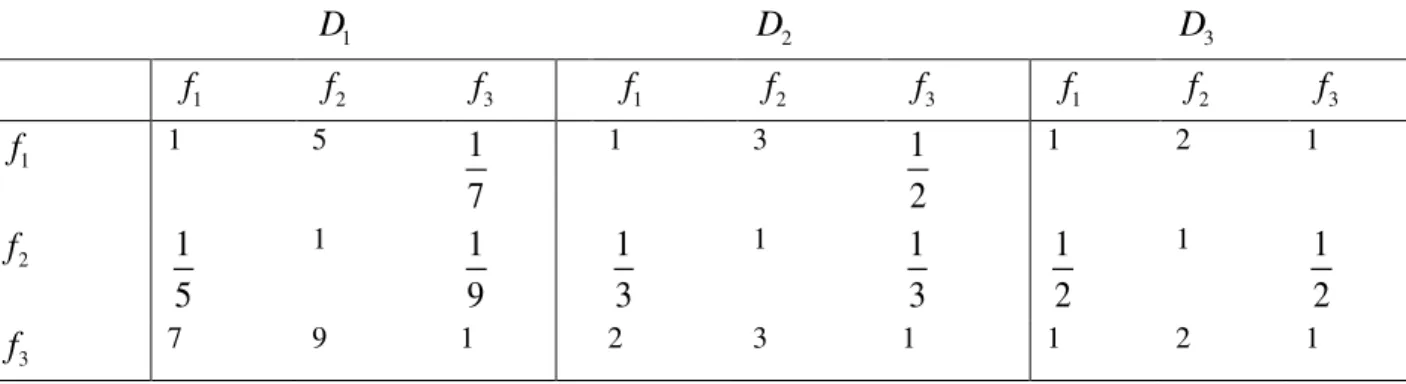
In order to determine the importance of objectives, each decision maker gives a pair-wised comparison matrix. Table 3 shows the pair-wised comparison matrices made by decision makers.

Table 3: The pair-wised comparison matrices for objectives.

1

D

₂

D

₃

1

f

₂

f

₃

f

₁

f

₂

f

₃

f

₁

f

₂

f

₃

1

f

1 5

₁

7

1 3

₁

2

1 2 1

2

f

1

5

1

₁

9

1

3

1

₁

3

1

2

1

₁

2

3

f

7 9 1 2 3 1 1 2 1

Step 1. Determining weights of DMs

We calculate the average pair-wised comparison matrix of group decision as the ideal pair-wised comparison matrix. Let t

 

t

ij _{n n}

A a



 be the pair-wised comparison matrix of th DM, and

1

1 3

k _t t

A



_ A where

1

1 3

k t ij _t ij

a



_ a

be the ideal pair-wised comparison matrix that shown as follows:

 

0.3441 3.3331 0.5480.944

3.333 4.667 1

ij

A a

 

 

 _{ } _

 

  (5.31)

In order to measure decision level of each DM, we can calculate the distance between each individual pair-wised comparison matrix

A

t and the ideal pair-wised comparison matrix

A

. The separation of each individual decision

A

tform the

A

, is given as:

Table 4: Separation of each individual decision

A

tform the

A



1

A

2

A

3

t

(16)

Now we calculate the two negative ideal solutions (NISs) namely L-NIS

A

l and R-NIS

A

ras follows:

 

0.21 21 0.1430.111

1 2 1

l l ij

A a

 

 

 _{ } _

 

  (5.32)

and

 

0.5 11 5 0.51

7 9 1

r r ij

A a

 

 

 _{ } _

 

  (5.33)

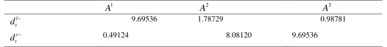
Similarly, the separations of each individual decision form the NISs, d_tl and d_tr, are given as Table 5.

Table 5: Separation of each individual decision

A

t_{form the negative ideal solutions}

1

A

_A

2

_A

3

l t

d  9.69536 1.78729 0.98781

r t

d  0.49124 8.08120 9.69536

The closeness coefficient of DMs with respect to

A

is calculated as Table 6:

Table 6: Closeness coefficient of DMs 1

A

2

A

3

t

R

0.62971 0.81463 0.73551

The weight of each decision maker is calculated as Table 7:

Table 7: Weight of each decision maker

1

D

₂

D

₃

t



0.28888 0.37371 0.33741

Step 2. Aggregating of Individual Judgments

We obtain a group judgment matrix (group pair-wised comparison matrix)

A



 

a

ij _{n n}_ as follows:

 

0.350931 3.240351 0.565570.32522

3.10699 4.39587 1

ij

A a

 

 

 _{ } _

 

  (5.34)

Step 3. Calculating the weight vector of objectives.

The weight of objectives is calculated by the AHP method. The results are shown in Table 8:

Table 8: Weights of objectives

1

f

₂

f

₃

j

(17)

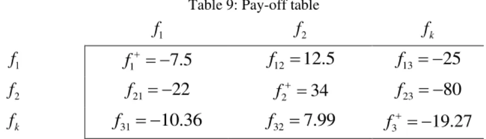
Step 4. Construct the pay-off table.

For this purpose we first maximize each objective function and construct a pay-off table to obtain the positive ideal criterion vector

f





R

k. The results are shown in Table 9:

Table 9: Pay-off table

1

f

₂

f

_k

1

f

f₁ 7.5

f

12



12.5 f

13

 

25

2

f

₂₁

 

22

f₂ 34

f

23

 

80

k

f

₃₁

 

10.36 f

₃₂



7.99

f₃  19.27

Step 5. Calculate the weight factors.

Since f₁ 7.5 and f₁min  22 and

c

₁₁

 

5,

c

₁₂



2 and

c

₁₃

 

3

then from formula (4.21) we have:





1

2 2 2 ₂

1

22 ( 7.5)

( 5)

2 ( 3)

0.107

22 





_

  



_





 











Similarly, we can obtain



2



0.108

and



3



0.067

. From formula (4.22) the weigh factors are obtained

as:

1 2 3

0.107 0.379 and

0.383 and

0.238 0.107 0.108 0.067















Now we can start the iteration process. We can obtain a criterion vector which is closest to positive ideal one and emphasize that more important objectives be more closer to ideal one by solve model (5.35) as follows:

1 2 3

(0)

min

. .

(0.2936)(0.379)( 7.5 5

2 3 )

,

(0.1198)(0.383)(34 3

4 5 )

,

(0.5866)(0.238)( 19.27 2

5 10 )

,

0 s t

x

S

R



























 

(5.35)

The optimal solution of the problem is

x

(0)



(0, 0, 2.615)

with criterion vector

(0)

(

)

( 7.84425,13.07375, 26.1475)

f x

 



.

(18)

1 1 2 3

(1) (0)

2 1 2 3 2

3 1 2 3

( ) 5 2 3 7.84425,

( ) 3 4 5 13.07375 ,

( ) 2 5 10 26.1475,

f x x x x

S x S f x x x x f

f x x x x

     

 

 

_         _

 _ _ _ _{ } 

  (5.36)

We set



₂



0

. Therefore we have



₂



0

and then we begin iteration 2.

It is obvious that



₁



0.615

,



₃



0.315

and we go to step 6.

We try to obtain a criterion vector which is closest to positive ideal one and emphasize that more important objectives be more closer to ideal one by solve model (5.37) as follows:

1 2 3

min

. .

(0.2936)(0.615)( 7.5 5

2 3 )

,

(0.5866)(0.385)( 19.27 2

5 10 )

,

5

2

3 7.84425,

3

4

5 10.07375,

2

5

10 26.1475,

s t

x

























 











 

(1)

,

0 x

S

R





 

(5.37)

x

(1)



(0.098, 0, 2.451)

(1)

(

)

( 7.843,11.961, 24.314)

f x

 



.

The results

x

(1)



(0.098, 0, 2.451)

and

f x

(

(1)

)

 

( 7.843,11.961, 24.314)



are shown to the decision maker. Suppose the solution is not satisfied as f x₃( (1)) 24.314 is too small. Suppose

f x

₁

( )

can be sacrificed by 3 units, or

 

f

₁

3

. Then the new search space is given by:

1 1 2 3 1

(2) (1)

2 1 2 3

3 1 2 3

( ) 5 2 3 7.843 ,

( ) 3 4 5 10.07375,

( ) 2 5 10 24.314,

f x x x x f

S x S f x x x x

f x x x x

       

 

 

_       _

 _ _ _ _{ } 

  (5.38)

(19)

It is obvious that



3



1

and we go to step 6.

We can obtain a criterion vector which is closest to positive ideal one and emphasize that more important objectives be more closer to ideal one by solve model (5.39) as follows:

1 2 3

(2)

min

. .

(0.5866)( 19.27 2

5 10 )

,

5

2

3 10.843,

3

4

5 10.07375,

2

5

10 24.314,

,

0 s t

x

S

R















 











 



 

(5.39)

x

(2)



(0.441, 0, 2.279)

(2)

(

)

( 9.042,10.072, 21.908)

f x

 



.

Note that,

x

(2)is the point in feasible region whose criterion vector has minimum distance to positive ideal and cause to objective

f x

2

( )

be more closer to ideal one.

According to the behavioral assumptions of the STEM method (discussed in decision phase), in this example the decision maker is satisfied with the solution

x

(2).

For problems having more than three objectives. In such circumstances, whether the decision maker is satisfied with a solution depends on the range of solutions he has investigated. Also, the sacrifices of multiple objectives should also be investigated in addition to the sacrifice of a single objective at each iteration.

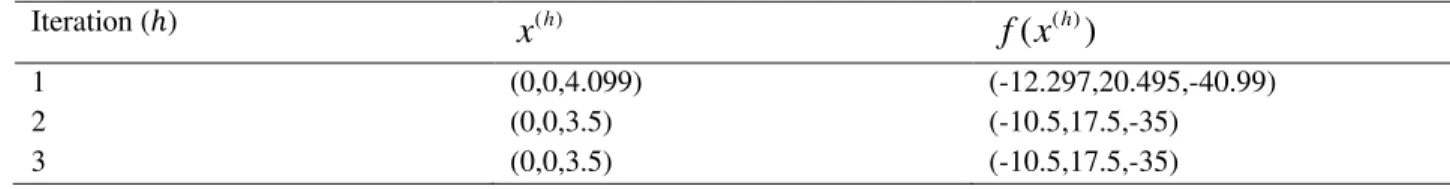
5.3. Solve with the classic STEM method

Suppose we want to solve the above problem with the classic STEM method. Therefore the iterations of solving this problem are as Table (10):

Table 10: The results of STEM method.

Iteration ( ) ( )h

x

f x

(

( )h

)

1 (0,0,4.099) (-12.297,20.495,-40.99)

2 (0,0,3.5) (-10.5,17.5,-35)

(20)

In iteration 2, we set

 

f

₂

3

and in iteration 3 we set

 

f

₁

3

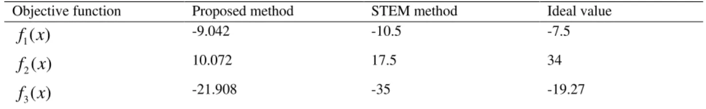
. By comparing with the results of proposed method, we can see that the optimal objective 3, (that is important than others) is closer to ideal objective. Similar is true for other objectives. See Table (11).

Table 11: Comparing between proposed method and STEM method

Objective function Proposed method STEM method Ideal value

1

( )

f x

-9.042 -10.5 -7.5

2

( )

f x

10.072 17.5 34

3

( )

f x

-21.908 -35 -19.27

From Table (11), it is obvious that, by considering the importance of objective functions, the proposed method obtains the better results.

6 Conclusion

The suggested method in this paper improves the STEM method by calculating the weight vector of objectives. These weights are such that, they emphasize that the more important objectives be closer to ideal one. For the purpose of finding these weights we apply the AHP and TOPSIS method by developing an integrated multi-objective group decision making procedure. Therefore, we find a point in reduced feasible region whose criterion vector is closest to positive ideal criterion vector and also, more important objectives are closer to ideal one. We solved a multi-objective decision making problem by both classic and proposed methods. In Table () we saw that the proposed method obtains the better results. Therefore the presented method increases the rate of satisfactoriness of the obtained solution.

References

[1] A. P. Agalgaonkar, S. V. Kulkarni, S. A. Khaparde, Evaluation of configuration plans for DGs in developing countries using advanced planning techniques, IEEE Transaction on Power Systems, 21 (2) (2006) 973-981.

http://dx.doi.org/10.1109/TPWRS.2006.873420

[2] J. Andersson, J. Pohl, P. Krus, Design of objective functions for optimization of multi-domain systems, presented at ASME Annual Winter meeting, FPST Division, Anaheim, California, USA, (1998).

[3] R. J. Balling, J. Richard, Pareto sets in decision-based design, Journal of Engineering Valuation and Cost Analysis, 3 (2) (2000) 189-198.

[4] R. J. Balling, Design by shopping: A new paradigm? in 3rdWorld Congress of Structural and Multidisciplinary Optimization, Buffalo, NY, May 1721, (1999).

[5] V. Belton, A comparison of the analytic hierarchy process and a simple multi-attribute value function, European Journal of Operational Research, 26 (1986) 7-21.

http://dx.doi.org/10.1016/0377-2217(86)90155-4

[6] R. Benayoun, J. De Montgolfier, J. Tergny, O. Laritchev, Linear programming with multiple objective functions: Step Method (STEM), Mathematical Programming, 1 (1971) 366-375.

(21)

[7] A. Charnes, W. W. Cooper, Management models and industrial applications of linear programing, John Wiley & Sons, New York, (1961).

[8] A. Charnes, W. W. Cooper, R. O. Ferguson, Optimal Estimation of executive compensation by linear programing, Management Science, 1 (1955) 138-151.

http://dx.doi.org/10.1287/mnsc.1.2.138

[9] S. J. Chen, C. L. Hwang, Fuzzy Multiple Attribute Decision Making: Methods and Applications, Springer-Verlag, Berlin, (1992).

http://dx.doi.org/10.1007/978-3-642-46768-4

[10] M. Chiampi, G F., Ch M., C R., M. R., Multiobjective optimization with stochastic algorithms and fuzzy definition of objective function, International Journal of Applied Electromagnetics in Materials, 9 (1998) 381-389.

[11] M. Chiampi, C. Ragusa, M. Repetto, Fuzzy approach for multiobjective optimization in magnetics, IEEE transaction on magnetics, 32 (1996) 1234-1237.

http://dx.doi.org/10.1109/20.497467

[12] W. A. Crossley, A. M. Cook, D. W. Fanjoy, V. B. Venkayya, Using the two branch tournament genetic algorithm for multiobjective design, AIAA Journal, 37 (2) (1999) 261-267.

http://dx.doi.org/10.2514/2.699

[13] I. Das, J. Dennis, Normal-boundary interaction: A new method for generating the Pareto surface in nonlinear multicriteria optimization problems, SIAM Journal of Optimization, 8 (1998) 631-657.

http://dx.doi.org/10.1137/S1052623496307510

[14] Y. Dong, G. Zhang, W-C. Hong, Y. Xu, Consensus models for AHP group decision making under row geometric mean prioritization method, Decision Support Systems, 49 (2010) 281-289.

http://dx.doi.org/10.1016/j.dss.2010.03.003

[15] C. L. Hwang, A. S. M. Masud, Multiple objective decision making Methods and applications: A state of- the-art survey, Lecture Notes in Economics and Mathematical Systems, Springer-Verlag: Berlin, 164 (1979).

http://dx.doi.org/10.1007/978-3-642-45511-7

[16] C. L. Hwang, K. Yoon, Multiple Attribute Decision Making: Methods and Applications - A State-of-the-Art Survey, Springer-Verlag, Berlin, (1981).

http://dx.doi.org/10.1007/978-3-642-48318-9

[17] I-J. Jeong, K-J. Kim, D-STEM: a modified step method with desirability function concept, Computers & Operations Research, 32 (2005) 3175-3190.

http://dx.doi.org/10.1016/j.cor.2004.05.006

[18] J. Jeonghwan, L. Rothrock, P. L. McDermott, M. Barnes, Using the Analytic Hierarchy Process to Examine Judgement Consistency in a complex multiattribute task, IEEE Transactions on Systems, Man and Cybernetics, Part A: Systems and Humans, 40 (2010) 1105-1115.