GROUNDWATER QUALITY, VULNERABILITY AND POTENTIAL ASSESSMENT IN KOBO VALLEY DEVELOPMENT PROJECT, ETHIOPIA

GROUNDWATER QUALITY, VULNERABILITY AND

POTENTIAL ASSESSMENT IN KOBO VALLEY

DEVELOPMENT PROJECT, ETHIOPIA

GROUNDWATER QUALITY, VULNERABILITY AND

POTENTIAL ASSESSMENT IN KOBO VALLEY

DEVELOPMENT PROJECT, ETHIOPIA

Dissertation supervised by

Professora Doutora Ana Cristina Costa, Ph.D

Coordinator of the Teaching Quality Assurance System

NOVA Information Management School

Universidade Nova de Lisboa, Portugal

Professor Jorge Mateu, Ph.D

Full Professor of Statistics

Department of Mathematics

Universitat Jaume I, Castellón, Spain

Sara Ribeiro,MSc

Researcher, NOVA Information Management School

Universidade Nova de Lisboa, Portugal

ACKNOWLEDGMENTS

I am very grateful to my supervisor Professor Ana Cristina Costa, Ph.D for being

always available throughout the whole thesis work. Without her constant support,

insightful comments, constructive criticisms and inspiring guidance, this thesis work

wouldn’t come to an end.

I also want to express my sincere gratitude to my co-supervisors Professor Jorge

Mateu, Ph.D and Engineer Sara Ribeiro for their timely follow up, advice, suggestions

and comments to shape the thesis work from the start to the end.

I owe my deepest gratitude to Professor Marco Painho, Ph.D for all the friendly and

fruitful discussions in the thesis work as well as in the Masters course.

Special thanks go to my colleague Habtamu Wagaw Mengistu (Geologist) for his

unlimited effort, devotion and professional opinion on the thesis work.

I would like to thank also Zebene Lakew, a Hydro geologist in the Ethiopian Ministry

of Water and Energy, for providing me the appropriate data and his continuous

communication throughout the thesis work.

Last but not least, I am very grateful to have a great family with enormous support,

GROUNDWATER QUALITY, VULNERABILITY AND

POTENTIAL ASSESSMENT IN KOBO VALLEY

DEVELOPMENT PROJECT, ETHIOPIA

ABSTRACT

This study deals with investigating the groundwater quality for irrigation purpose, the

vulnerability of the aquifer system to pollution and also the aquifer potential for

sustainable water resources development in Kobo Valley development project. The

groundwater quality is evaluated up on predicting the best possible distribution of

hydrogeochemicals using geostatistical method and comparing them with the water

quality guidelines given for the purpose of irrigation. The hydro geochemical

parameters considered are SAR, EC, TDS, Cl

, Na

, Ca

, SO

and HCO

. The

spatial variability map reveals that these parameters falls under safe, moderate and

severe or increasing problems. In order to present it clearly, the aggregated Water

Quality Index (WQI) map is constructed using Weighted Arithmetic Mean method. It

is found that Kobo-Gerbi sub basin is suffered from bad water quality for the irrigation

purpose. Waja Golesha sub-basin has moderate and Hormat Golena is the better

sub basin in terms of water quality. The groundwater vulnerability assessment of the

study area is made using the GOD rating system. It is found that the whole area is

experiencing moderate to high risk of vulnerability and it is a good warning for proper

management of the resource. The high risks of vulnerability are noticed in Hormat

Golena and Waja Golesha sub basins. The aquifer potential of the study area is

obtained using weighted overlay analysis and 73.3% of the total area is a good site

for future water well development. The rest 26.7% of the area is not considered as a

good site for spotting groundwater wells. Most of this area fall under Kobo-Gerbi sub

KEYWORDS

WQI

GOD Rating System

Vulnerability

Geostatistical Method

Weighted Arithmetic Mean

Aquifer Potential,

Spatial Variability

ACRONYMS

B

-Boron

BK

-Bayesian Kriging

Ca

-Calcium

Cl

-Chloride

Co-SAERAR

- Commission for Sustainable Agriculture and

D

-Depth to Water Level

EC

-Electrical Conductivity

ENGDA

- National Groundwater Database Association

Environmental Rehabilitation of Amhara Region

FAO

-Food and Agricultural Organization

G

-Groundwater Occurrence

GIS

-Geographical Information System

H

-Aquifer Thickness

HCO3

-Bicarbonate

h

-Static Water Level

IDW

-Inverse Distance Weighting

ITCZ

- Inter-Tropical Convergence Zone

KCl

-Pottasium Chloride

KGVDP

-Kobo Girana Valley Development Project

K

-Hydraulic Conductivity

k

-Proportional Constant

MAE

-Mean Absolute Error

ME

-Mean Error

Meq

-miliequivalent

MS

-Matrix System

NaCl

-Sodium Chloride

Na

-Sodium

OK

-Ordinary Kriging

O

-Overlying Lithology

PCSM

-Point Count System Model

RBF

- Radial Basis Functions

RMSE

-Root Mean Square Error

RSC

-Residual Sodium Carbonate

SAR

-Sodium Adsorption Ratio

SO4

-Sulphate

STL

-Static Water Level

TDS

-Total Dissolved Solids

T

-Transmitivity

UK

-Universal Kriging

UTM

-Universal Transverse Mercator

WAWQI

- Weighted Arithmetic Water Quality Index

WHO

-World Health Organization

Wi

-weight of parameter

INDEX OF THE TEXT

ACKNOLEDGEMETS………iii

ABSTRACT……….iv

KEYWORDS………...v

ACRONYMS………...vi

INDEX OF TEXTS………viii

INDEX OF TABLES………...x

INDEX OF FIGURES………xi

1.Introduction...1

1.1 Statement of the problem ... 3

1.2 Objectives of the study ... 3

1.3 Research Questions ... 4

1.4 Methodological framework... 4

1.5 Thesis organization ... 4

2. Literature Review………...5

2.1 General ... 5

2.2 Groundwater for Irrigation Purpose ... 7

2.3 Effects of Soluble Salts on Plants ... 10

2.3.1 Salinity hazards and water deficiency ... 10

2.3.2 Toxicity hazards ... 11

2.4 Effects of soluble salts on soil ... 11

2.4.1 Sodium hazard ... 11

2.4.2 Residual sodium carbonate (RSC) ... 11

2.5 Water Quality Indices ... 12

2.5.1 General ... 12

2.5.2 Arithmetic Water Quality Index ... 13

2.6 Groundwater Vulnerability to Pollution ... 13

2.6.1 General ... 13

2.6.2 GOD Rating System ... 14

2.6.3 DRASTIC Method ... 14

2.7 Groundwater Potential of the Aquifer ... 15

3. Study Area………...16

3.1 General ... 16

3.2 Regional Geology and Hydrogeology ... 17

3.2.1 General Geology ... 17

3.4 Drainage System ... 23

3.4.1 General ... 23

3.4.2 Waja Golesha Sub Basin ... 23

3.4.3 The Kobo-Gerbi Closed Sub Basin ... 23

3.4.4 The Hormat Golina Sub Basin... 24

3.4.5 Groundwater Divide Line ... 25

4. Data and Methodology………...26

4.1 Data ... 26

4.1.1 Data Preparation ... 26

4.1.2 Data Cleaning ... 26

4.1.3 Data transformation ... 27

4.1.4 Exploratory Data Analysis ... 27

4.2 Methodology ... 31

4.2.1 Interpolation Methods ... 31

4.2.2 Variogram ... 34

4.2.3 General Procedure ... 36

5. Results and Discussion………...40

5.1 Variogram Analysis ... 40

5.2 Groundwater Parameters Surfaces ... 40

5.2.1 Groundwater Quality Parameters ... 42

5.2.2 Water Quality Index (WQI) ... 52

5.2.3 Ground Water Pollution Index ... 54

5.2.4 Groundwater Potential ... 57

6. Conclusions and Recommendations………...60

6.1 Conclusion ... 60

6.2 Recommendations ... 60

References………....61

Annexes……….67

A.1 Histograms of Groundwater Parameters ... 67

A.2 Normal QQ Plot of Groundwater Quality Parameters……….69

A.3 Maps generated for each prediction methods ... 72

A.4 Cross Validation Results ... 80

A.5 Maps of aquifer parameters ... 81

A.6 GOD Flow Chart for Vulnerability Assessment (Foster, 1987). ... 82

A.7 Kobo Monthly Rainfall (mm) ... 83

A.8 Variogram Analysis for groundwater parameters ... 83

A.9 Water Quality Data... 87

INDEX OF TABLES

Table 2.1: Major, Secondary and Trace constituents of Groundwater (Source: Harter,

2003)...8

Table 3.1 climate regions as per rainfall coeficient (Source: Daniel Gemechu,

1977)…...22

Table 3.2 Areal Coverages of Sub-Basins in Kobo Girana valley (Source:Metaferia

ConsultingEngineers,2009)…………...23

Table 4.1 Descriptive Statistics of groundwater parameters...28

Table 4.2 Correlation coefficient values of the groundwater quality parameters...29

Table 5.1: Model fits and their parameters………...40

Table 5.2: Best surface prediction methods...41

Table 5.3 Guideline of SAR for irrigation purpose (Bara, 2008)...42

Table 5.4 guideline for chloride concentration in irrigation water (Mass, 1990)...47

Table 5.5 weights of groundwater quality parameters...53

Table 5.6 Classification of water quality index and percent area coverage...54

Table 5.7 Ranges and ratings of G, O, and D parameters...55

Table 5.8 Vulnerability scale as of GOD rating system (Foster, 1987)...55

Table 5.9 Pollution potential percentage in the study area...57

Table 5.10 Weights and rates of aquifer parameters for aquifer potential site

assessment...58

INDEX OF FIGURES

Figure 3.1 Location of the study area(Metaferia Consulting Engineers,2009)……….16

Figure3.2 Geology and Structural Map of Kobo-Girana valley: source geological map

of Ethiopia, 1996………...19

Figure3.3 Geology of Kobo Valley (Source: Metaferia Engineering, 2009)………….20

Figure3.4 Drainage system map of the sub-Basins in Kobo Girana Valley (Source:

Metaferia Consulting Engineers, 2009)………...24

Figure 3.5

Groundwater Divide Line of Kobo Valley (Metaferia Consulting Engineers,

2009)...25

Figure 4.1 Typical Semivariogram: Source (Bohling, 2005)………...34

Figure 4.2 General Methodology...39

Figure 5.1 Spatial Distribution of SAR...43

Figure 5.2 Spatial Distribution of TDS...44

Figure 5.3 Spatial Distribution of EC...45

Figure 5.4 Spatial Distribution of Na...47

Figure 5.5 Spatial Distributions of Chloride...49

Figure 5.6 Spatial Distributions of Ca...50

Figure 5.7 Spatial Distribution of sulphate...51

Figure 5.8 Spatial Distribution of Bicarbonate...52

Figure 5.9 Water Quality Index map of the study area...54

Figure 5.10 God Vulnerability map...56

1. Introduction

Most of the Earth’s liquid fresh water is found, not in lakes or rivers, but is stored underground in the aquifers. Indeed, these aquifers provide a valuable base flow supplying water to rivers during periods of no rainfall. They are therefore an essential resource that requires protection so that groundwater can continue to sustain the human race and the various ecosystems that depend on it. The contribution from groundwater is vital; according to Morris and et.al, two billion people depend directly upon aquifers for drinking water, and 40 percent of the world‘s food is produced by irrigated agriculture that relies largely on groundwater. In the future, aquifer development will continue to be fundamental to economic development and reliable water supplies will be needed for domestic and irrigation purposes. Water stored in the ground beneath our feet is invisible and so its depletion or degradation due to contamination can proceed unnoticed, unlike our rivers, lakes and reservoirs, where drying up or pollution rapidly becomes obvious and is reported (Morris et al. 2003).

Hydro geologic or ground water parameters include the depth of the water level measured in the observation wells, the quantity or discharge of the aquifer, the water quality of the water bearing stratum, the hydraulic permeability of the aquifer, etc. The sustainable use of groundwater resource is the properly management of groundwater related phenomenon for the wise use of the resource. By knowing the depth of ground water level in a certain area, one might be able to observe how depleted the aquifer system is. At the same time, by monitoring the quality of the water, it is possible to adopt mechanisms to mitigate or take actions. The other parameter for the indication of groundwater quantity and also for groundwater pollution is the permeability of the groundwater aquifer. The higher the permeability of the aquifer, the higher the yield will be so that it may be used to locate relative potential areas with the help of other parameters like aquifer thickness, the hydro geological make up of the area, and the depth to the static water table, etc. There are ranges of values for which we say the aquifer is a good one based on the factors considered.

patterns, ranging from traditional stream gauging to remote sensing. Ideally, a measurement technique should be designed to take into account the type of natural variability one would expect to encounter. Depending on the nature of the hydrological variability, certain measurement techniques will be more suitable than others (Grayson and Bloschl, 2000).

Although there are perennial rivers and other intermittent streams in Kobo valley, the use of the groundwater resources is found to be crucial for the development of irrigation agriculture in the project area. This is because of the available land resource for irrigation in the project area is vast and could not be covered with the existing surface water resource (Feasibility Study Report of KGVDP, Volume II: Hydrology,1999).

Irrigation water increases crop yields and quality in semi arid areas like Kobo, in the Northern part of Ethiopia. Irrigation is essential especially during periods of erratic rainfall and drought. Since there is a degradation of the groundwater, which is the main source of irrigation in the area, the irrigation water efficiency has to be increased as much as possible (Adane, 2014). From the above statement, it is evident that management of those resources is vital to make the inflow and outflow proportional to sustain future expansion and sustainability.

The groundwater table in Kobo-Girana is supplied by recharge from the areal rainfall and lateral recharge from the surrounding mountains. This makes the area higher groundwater potential. In the country, this is the only project significantly benefited from groundwater irrigation. According to hydro geological investigation report by Metaferia Consulting Engineers (2009), a certain portion of the groundwater potential of the valley is the reserved groundwater. Therefore caution is needed to sustain use of the available groundwater.

There is large amount of irrigable land but the current irrigated area is very small for different reasons. Farmers and regional government are trying to drill more deep wells to cover the whole irrigable land in the valley (Endalamaw, 2009).

Finding groundwater, in basins such as Kobo Girana, is not the problem. Just dig and you will eventually find it. The real challenge faced by the exploration hydro geologist is to site and design high yield wells (Ferriz and Bizuneh, 2003). And identification of areas with high aquifer permeability might be helpful as a supplementary source in the geological investigation of future borehole spots.

Due to the volcanic geological formation of the area and the surroundings, the ground water aquifer consists of different hydrogeochemicals. The quality of the groundwater may also be deteriorated due to pumping from wells. In addition to this, the chemicals used as fertilizer in the irrigation system can percolate down to the aquifer.

random locations (Kitanidis, 1997). Geostatistics offers a variety of tools including interpolation, integration and differentiation of hydro geologic parameters to produce the prediction surface and other derived characteristics from measurements at known locations. In this work, Geostatistcs techniques are going to be used as a modelling tool for analysing the spatial variation of different groundwater parameters in Kobo Valley Development Project. This study is beneficial to know the groundwater system for better utilization and management of the resources.

1.1 Statement of the problem

Kobo Girana Basin is one of the areas in Ethiopia with significant reserved groundwater potential. Yet, the area has suffered from erratic rainfall and is of a drought prone. The source of water for irrigation and domestic purpose is the reserved groundwater. With increasing number of population and demand for agricultural products, the sustainable use of this resource is paramount. It is has been reported that in some areas due to the application of chemicals like fertilizers, weed removal and the geological makeup of the area (the interaction between the rock and the water), the water quality is being threatened (Metaferia Consulting).

The other challenging problem to the hydro geologist was spotting the high yielding aquifer parts in the area with less cost. This is due to the fact that the area has a complex geological formation.

Due to the above problems, Geostatistical methods of prediction for hydro geochemical properties (groundwater quality) and the better groundwater potential sites based on the aquifer properties are proposed to be done for controlling and managing the groundwater system by informing the outcome to the respected body or organization.

1.2 Objectives of the study

• To study the spatial variability of hydro geochemical properties (groundwater quality

) of the study area

• To study the vulnerability of the area to pollution.

• To study the groundwater potential for spotting high yielding aquifers sites for future

development.

1.3 Research Questions

The following research questions can be drawn

• How is the distribution of hydro geochemical properties of the aquifer system?

• Which part of the study area has more potential to pollution?

• Where are the probable high yielding aquifer spots?

1.4 Methodological framework

In order to achieve the objectives stated in section 1.2, a certain methodological framework is followed. Geostatistical (Ordinary, Universal and Bayesian Kriging) and Inverse Distance Weighting methods are used to develop the best possible maps of several groundwater quality and aquifer parameters. Each parameter is evaluated against the four prediction methods to get the best possible spatial distribution using the cross validation. Up on getting the best possible spatial distribution of each groundwater quality parameters, the Water Quality Index (WQI) map is developed. The weighted arithmetic mean method is used to obtain the water quality index map. For assessing the vulnerability of the study area for pollution, GOD rating system that uses aquifer parameters as inputs is used. Furthermore, the groundwater potential map of the study area which can be used to spot the drilling sites for future development is made using weighted overlay analysis.

1.5 Thesis organization

2. Literature Review

2.1 General

In applied statistical modelling (including regression and time-series) least squares or linear estimation is the most widely used approach. The Advanced adoption of such methods is well suited to the solution of estimation problems involving quantities that vary in space. Examples of such quantities are conductivity, hydraulic head, and solute concentration. This approach is known as the theory of regionalized variables or simply geostatistics. It was popularized in mining engineering in 1970s and now it is used in all fields of earth science and engineering particularly in the hydrologic and environmental fields. Geostatistics is well accepted among practitioners because it is a down-to-earth approach to solve problems encountered in practice using statistical concepts that were previously considered recondite (Kitanidis, 1997).

An important distinction between geostatistical and conventional mapping of environmental variables is that the geostatistical prediction is based on application of quantitative, statistical techniques. Unlike the traditional approaches to mapping, which rely on the use of empirical knowledge, in the case of geostatistical mapping we completely rely on the actual measurements and (semi-)automated algorithms. Although this sounds as if the spatial prediction is done purely by a computer program, the analysts have many options to choose whether to use linear or non-linear models, whether to consider spatial position or not, whether to transform or use the original data, whether to consider multicolinearity effects or not. So it is also an expert-based system in a way (Hengl, 2007). It typically comprises of the following five steps:

1. design the sampling and data processing, 2. collect field data and do laboratory analysis, 3. analyse the points data and estimate the model, 4. implement the model and evaluate its performance, 5. Produce and distribute the output geoinformation.

The natural resource inventories need to be regularly updated or improved in detail, which means that after step (5), we often need to consider collection of new samples or additional samples that are then used to update an existing GIS layer (Hengl, 2007). For this proposed study, works related to spatial variability of groundwater parameters, vulnerability assessment and groundwater potential are reviewed.

Valley. The objective of his study was to quantify the recharge and abstraction of groundwater.

The other study was done by Endalamaw in 2009.He has done a work on optimum utilization of groundwater in Kobo valley. The work mainly focuses on quantifying annual recharge and status of the groundwater table using water balance equations under different scenarios of pumping and recommends that the groundwater should be managed for sustainability.

Gundogdu and Guney (2007) made spatial analysis of groundwater level using Universal Kriging. In this study, they were trying to find the best empirical semivariogram models that matched with the experimental models. They found out that the rational quadratic empirical semivariogram is the best fitted model.

Sahoo and Jha (2014) have done Analysis of Spatial Variation of Groundwater Depths Using Geostatistical Modelling. Groundwater depth data of 24 observation wells in the study area for 15 year period (1997-2011) were considered for the analysis. Ordinary kriging method was considered to evaluate the accuracy of the selected variograms in the estimation of the groundwater depths. The analysis of results indicated that geostatistics can reveal stochastic structure of groundwater level variations in space. Spatial analysis showed a significant groundwater fluctuation in the study area. The exponential model was found to be the best-fit geostatistical model for the study area, which were used for developing contour maps of pre- and post-monsoon groundwater depth.

Ahmadi and Sedghamiz (2007) analyzed the spatial and temporal variation of the groundwater level using Universal and Ordinary Kriging methods on 39 peizometric wells for a duration of 12 years. The years considered are 1993 and 2004.Variaogram models were developed and the prediction performances were checked with cross-validation. Both Ordinary and Universal Kriging methods yield good results with very small errors.

Moradi et al. (2012) conducted a study on Geostatistics approaches for Investigation of aquifer Hydraulic Conductivity in Shahrekord Plain, Iran. The purpose of this study is the investigation of spatial changes of hydraulic conductivity. Kriging, Inverse Distance Weighting method (IDW), Local Polynomial Interpolation and Global Polynomial Interpolation methods were used for interpolation. Well hydraulic Conductivity data were considered. Ordinary Kriging was found to be the best method of interpolation.

fitted well in the spherical for water depth and in the exponential model for the water quality (electrical conductivity).

Patriarche (2005) made a geostatsitical estimation of hydraulic conductivity at the Carrizo aquifer,Texas. Two different approaches were used to determine the hydraulic conductivity of the area. The first is an indirect method where hydraulic conductivity (K) is determined from Transmitivity (T). The other approach is a direct method where hydraulic conductivity can be kriged. Simple Kriging, Ordinary Kriging, Kriging with an external drift and Co-Kriging were used for the prediction of the surfaces under different sclaes of the area ( model,country and Texas domains). Prediction performances were assesed through cross validation.In the small model domain area for the indirect method, simple kriging gave better results. For larger regional scales for the same indirect method,Co-Kriging gave better reults. For the direct approach, the best prediciton performance was obtained using Kriging with an external drift.

The above sample works confirm that geostatistical methods can be used in the prediction of environmental variables like water quality, hydraulic permeability, transmissivity, groundwater depth, etc.

2.2 Groundwater for irrigation purpose

Irrigation water whether derived from springs, diverted from streams, or pumped from wells, contain appreciable quantities of chemical substances in solution that may reduce crop yield and deteriorate soil fertility. In addition to the dissolved salts, which has been the major problem for centuries, irrigation water always carry substances derived from its natural environment or from the waste products of man’s activities (domestic and industrial effluents). These substances may vary in a wide range, but mainly consist of dirt and suspended solids resulting into the emitters’ blockages in micro-irrigation systems and bacteria populations and coliforms harmful to the plants, humans and animals (Ayers, 1976).

The most damaging effects of poor-quality irrigation water are excessive accumulation of soluble salts and/or sodium in soil. Highly soluble salts in the soil make soil moisture more difficult for plants to extract, and crops become water stressed even when the soil is moist. When excessive sodium accumulates in the soil, it causes clay and humus particles to float into and plug up large soil pores. This plugging action reduces water movement into and through the soil, thus crop roots do not get enough water even though water may be standing on the soil surface (Zhang,1990).

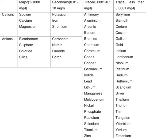
water quality parameters. Since most groundwater is colourless, odourless and without specific taste, we are typically more concerned with its chemical qualities (Harter, 2003). The lists of dissolved solids in natural ground water may be classified as major constituent, secondary constituent and trace constituents and are given in the Table 2.1 below.

Major(1-1000 mg/l) Secondary(0.01-10 mg/l) Trace(0.0001-0.1 mg/l)

Trace( less than 0.0001 mg/l) Cations Sodium

Calcium Magnesium Potassium Iron Strontium Antimony Aluminium Arsenic Barium Bromide Cadmium Chromium Cobalt Copper Germanium Iodide Lead Lithium Manganese Molybdenum Nickel Phosphate Rubidium Selenium Titanium Zinc Beryllium Bismuth Cerium Cesium Gallium Gold Indium Lanthanum Niobium Platinum Radium Ruthenium Scandium Silver Thallium Thorium Thin Tungsten Ytterbium Yttrium Zirconium Anions Bicarbonate

Sulphate Chloride Silica Carbonate Nitrate Fluoride Boron

Table 2.1 Major, Secondary and Trace constituents of Groundwater (Source: Harter, 2003)

The salinity hazard can be estimated by measuring the electrical conductivity (EC) directly or the Total Dissolved Solid (TDS). Electrical conductance, or conductivity, is the ability of a substance to conduct an electric current. The presence of charged ionic species in solution makes the solution conductive. According to Ayers and Westcot (1994), EC (µS/cm) values less than 750, 750-3000 and greater than 3000 are categorized as none, medium, and severe salinity hazard respectively. With regards to TDS (mg/l), values less than 450, 450-2000 and greater than 450-2000 are grouped as none, medium and severe respectivley.

Beside the potential dangers from high salinity, sodium hazard sometime exists. The two principal effect of sodium are a reduction in soil permeability and a hardening of the soil. Both effect are caused by the replacement of calcium and magnesium ions by sodium ions on the soil clays and colloids. The extent of this replacement can be estimated by sodium adsorption ratio (SAR) which is expressed by the following given in Eq.2.1.

2

Mg

Ca

Na

SAR

+

=

Toxicity problems occur if certain (constituents) ions in the water are taken up by the plant and accumulate to concentrations high enough to cause crop damage or reduced yields.The ion toxicity may come from sodium (Na), chloride (Cl), Boron (B), Sulphate (SO4) and etc

(Ayers and Westcot, 1994).

Marko and et al (2013) studied Geostatistical analysis using GIS for mapping groundwater quality (case study in the recharge area of Wadi Usfan, Western Saudi Arabia). In their study; Ordinary kriging method was applied to map the spatial distribution of the groundwater chemistry. And they came up with the conclusion that most of the groundwater is not suitable for drinking purposes based on the guidelines set for the purpose.

Rawat and et al. (2012) made a research entitled Spatial Variability of Ground Water Quality in Mathura District (Uttar Pradesh, India) with Geostatistical Method. In this study, kriging methods were used for predicting spatial distribution of some groundwater quality

parameters such as: Ca2+, Mg2+, Na+, K+, TDS, EC, Fˉ, HCO3ˉ, NO3ˉ, Clˉ, SO₄

2ˉ

and PO

4 2ˉ

.

methods were compared by the Root Mean Square Error (RMSE) and Mean Absolute Error (MAE). They obtained that Co-Kriging is the best method of prediction the groundwater quality in this study area.

Hassen (2014) conducted a study on the geostatistical analysis of groundwater quality in

Tehsil Sheikhupura region, Pakistan for better understanding of the distribution of each chemical element. The goestatistical analysis of the chemicals was performed and spatial distribution of maps was developed by Ordinary Kriging. The chemical concentrations were compared against the guidelines of WHO for drinking water.

Nas (2009) studied the groundwater quality for the purpose of drinking water. The Geostatistical Analyst extension module of ArcGIS was used in the study for exploratory data analysis, semivariogram, cross validation, mapping the spatial distribution of pH, electrical conductivity, Cl-, SO4-, hardness, and NO3- concentrations. The Ordinary Kriging method was

used to produce the spatial patterns of these chemical concentrations. The result showed there is high concentration of the chemicals on the north east part of the study area.

Anomohanran and Chapele (2012) made a study that evaluated the effectiveness of kriging interpolation technique for estimating permeability or hydraulic conductivity distribution by using 39 well data. The permeability obtained in the kriging method was compared with other empirical models and the error is found to be small ranging from 0.6 to 2.4%.

2.3 Effects of soluble salts on plants

The application of irrigation water to the soil introduces salts into the root zone. Plant roots take in water but absorb very little salt from the soil solution. Similarly, water evaporates from the soil surface but salts remain behind. Both processes result in the gradual accumulation of salts in the root zone. This situation may affect the plants in two ways: a) by creating salinity hazards and water deficiency; and b) by causing toxicity and other problems (Phocaides, 2000).

2.3.1 Salinity hazards and water Deficiency

and remains in the soil solution, while sulphate and bicarbonate combine with calcium and magnesium, where present, to form calcium sulphate and calcium carbonate, which are sparingly soluble compounds (Phocaides, 2000).

2.3.2 Toxicity hazards

Many fruit trees and other cultivations are susceptible to injury from salt toxicity. Chloride, sodium and boron are absorbed by the roots and transported to the leaves where they accumulate. In harmful amounts, they result in leaf burn and leaf necrosis. Moreover, direct contact during sprinkling of water drops with high chloride content may cause leaf burn in high evaporation conditions. To some extent, bicarbonate is also toxic. Other symptoms of toxicity include premature leaf drop, reduced growth and reduced yield. In most cases, plants do not show clear toxicity problems until it is too late to remedy the situation. Chloride and sodium ions are both present in the solution. Thus, it is difficult to determine whether the damage caused is due to the one or to the other. Chloride ions in high concentrations are known to be harmful to citrus and many woody and leafy field crops. Chloride content exceeding 10 meq/litre may cause severe problems to crops. The effect of sodium toxicity is not very clear. However, it has been found that it may cause some direct or indirect damage to many plants (Phocaides, 2000).

2.4 Effects of soluble salts on soil

2.4.1 Sodium hazard

A soil permeability problem occurs with high sodium content in the irrigation water. Sodium has a larger concentration than any other cation in saline water, its salts being very soluble. Positively charged, it is attracted by negatively charged soil particles, replacing the dominant calcium and magnesium cations. The replacement of the calcium ions with sodium ions causes the dispersion of the soil aggregates and the deterioration of its structure, thus rendering the soil impermeable to water and air. The increase in the concentration of exchangeable sodium may cause an increase in the soil pH to above 8.5 and reduce the availability of some micronutrients, e.g. iron and phosphorus.

The sodium problem is reduced if the amount of calcium plus magnesium is high compared with the amount of sodium. This relation is called the sodium adsorption ratio (SAR). The use of water with a high SAR value and low to moderate salinity may be hazardous and reduce the soil infiltration rate (Phocaides, 2000).

2.4.2 Residual sodium carbonate (RSC)

increases resulting in the dispersion of soil. When the RSC value is lower than 1.25 meq/litre, the water is considered good quality, while if the RSC value exceeds 2.5 meq/litre, the water is considered harmful (Phocaides, 2000).

2.5 Water Quality Indices

2.5.1 General

Groundwater quality parameters include the Sodium Adsorption Ratio (SAR), Total Dissolved Solids (TDS), Electric Conductivity (EC), Sodium (Na+), Calcium (Ca++), Chloride (Cl-), Sulphate (SO42-), Bicarbonate (HCO3-) ,Magnesium(Mg++) etc. In water quality analysis

using geostatistical methods, it is possible to make spatial analysis for each parameter and compare the values with the guidelines for irrigation purpose. It is expected that some of the parameters are within the guidelines and some

are

WQI is a mathematical instrument used to transform large quantities of water quality data into a single number which represents the water quality level while eliminating the subjective assessments of water quality and biases of individual water quality experts. Basically a WQI attempts to provide a mechanism for presenting a cumulatively derived, numerical expression defining a certain level of water quality (Miller et al., 1986).

Water Quality Indices can be classified in to two groups: objective or subjective. Objective methods are those which are not using subjective inferences. The indices obtained by subjective methods are often called statistical indices. In the subjective methods, the weights and ratings are entirely subjective and are drawn out of questionnaire analysis inquiring the opinion of experts. The advantage of objective over subjective is its unbiasedness (Ott, 1978).

2.5.2 Arithmetic Water Quality Index

This water quality index is an index originally proposed by Horton in 1965 and also called as the weighted arithmetic mean method. Many researchers like Brown et.al, 1970 and many more have used this index in their research work. Recently, Omran (2012), Ambica (2014), Chowdhurry et.al (2012) used the Weighted Arithmetic Mean method to assess the water quality index.

2.6 Groundwater Vulnerability to Pollution

2.6.1 General

Groundwater vulnerability index is the measure of the aquifer pollution potential based on some hydro geological, morphological and hydrographical parameters. It is not possible for directly measuring the groundwater vulnerability as of the water quality parameters in assessing the quality of water for a specific use.

Different methods are proposed by different researchers for assessing the vulnerability of groundwater for pollution. Parametric System method is one of them. This parameter system method intern has Matrix System (MS), Rating System (RS) and Point Count System Models (PCSM).And they are based on Overlay and Index method.

Ground water vulnerability assessment has the ability to delineate areas, which are more likely than others to become polluted as a result of anthropogenic activities at or near the land surface (Vrba and Zaporozec, 1994).

For all parametric system methods the procedure is almost the same. The system definition depends on the selection of those parameters considered to be representative for groundwater vulnerability assessment. Each parameter has a defined natural range divided into discrete hierarchical intervals. To all intervals are assigned specific values reflecting the relative degree of sensitivity to contamination (Gogu and Dassargues, 2000).

parameters. Rating parameters for each interval are multiplied accordingly with the weight factor and the results are added to obtain the final score. This score provides a relative measure of vulnerability degree of one area compared to other areas and the higher the score, the greater the sensitivity of the area. One of the most difficult aspects of these methods with chosen weighting factors and rating parameters remains distinguishing different classes of vulnerability (high, moderate, low etc.), on basis of the final numerical score. Examples are DRASTIC, SINTACS and EPIK methods (Gogu and Dassargues, 2000).

2.6.2 GOD Rating System

GOD rating system is an empirical method for assessing the vulnerability of the aquifer system. It only needs three parameters in order to get the result and it is simple. When there is a limitation in the data for using other methods like DRASTIC and others, this method is a good choice. The three parameters considered are Groundwater occurrence (G), Overlying aquifer litho logy (O) and Depth to the groundwater table (D). The ratings for each of the parameters and their classes are given by the GOD chart.

The vulnerability index is obtained by multiplying the groundwater occurrence ratings with the ratings of the overlaying aquifer litho logy and again with the ratings of the depth to the groundwater level. The index values are between 0 and 1. The higher the values, the more vulnerable the area is for pollution. The GOD Rating flow chart is shown in the Annex V.

2.6.3 DRASTIC Method

This method considers the following factors in order to determine the vulnerability of the aquifer pollution. Depth to Water(D), Recharge(R), Aquifer Media(A),Soil Media(S),Topography(T), Impact of the Vadose Zone(I) and Hydraulic Conductivity (C) of the Aquifer. These factors are arranged to for the acronym DRASTIC for ease of reference. A numerical ranking system to assess groundwater pollution potential in hydro geologic settings has been devised using the DRASTIC factors. The system contains three significant parts: weights, ranges and ratings. The weights are between 1 to 5 and individual parameters are assigned fixed values based on their influence. So, these weights are constant and cannot be changed. Then each parameter is classified in to certain ranges according to their impact on pollution potential. The range of each DRASTIC factor is rated between 1 to 10 (Aller et.al, 1985).

The equation for DRASTIC method is:

DrDw+RrRw+ArAw+SrSw+TrTw+IrIw+CrCw=Pollution Potential ...Eq. 2.2 Where r=rating

2.7 Groundwater Potential of the Aquifer

Groundwater potential sites are sites which have the appropriate conditions for yielding good quantity of water in the aquifer system . Different aquifer parameters like the thickness, hydraulic permeabilitity , geology of the overlaying aquifer and the depth to the static water table are some of the factors that might influence the existance of a good quantity of water in groundwater basin.

The type and number of themes used for the assessment of groundwater resources by geoinformatics techniques varies considerably from one study to another. In most studies, local experience has been used for assigning weights to different thematic layers and their features (Hutti et. al, 2011).

Amah et. al (2012) used some of the aquifer parameters to spot the good aquifer potential areas in Calabar coastal aquifer. They used litho logy, aquifer thickness, hydraulic conductivity or transmissivity, static water level and storativity to plot the final aquifer potential maps of the area.

3. Study Area

3.1 General

The Kobo valley is part of the Kobo Girana Valley Development Project in the North Eastern Amhara regional state, North Wollo Administrative Zone. The Kobo System and valley inter-mountain plain is between UTM 1300000 m - 1360000 m north, and UTM 540000 m- 582000 m east. The valley plain has an elongation in north-south direction. The valley is surrounded by Zoble Mountain in the east, the western escapement of the mainland in the west, Raya Valley in the North and volcanic ridges in the South. The study area is shown in the Figure 3.1 below. The Kobo catchment covers parts of three woredas, Kobo, Guba Lafto and Gidan. The valley is bounded by Zobil mountain ranges in the East & the North-Eastern escarpment in the West. The northern ridge of Girana valley namely Guba ridge and the Alamata Woreda bound the valley in the South and North respectively. The sub-basin is divided into Waja-Golelsha , Hormat-Golina and Kobo-Gerbi groundwater basins by undulating surfaces and volcanic inselbergs and intrusion lying in the east-west direction following the Kobo-Zobel road along Gara Lencha–Mendefera stretch.

3.2 Regional Geology and Hydrogeology

3.2.1 General Geology

The geology of north and central Ethiopia, which also includes the current study area, is dominated by Tertiary volcanic strata underlain by Mesozoic sedimentary rocks. The dominant outcrops on the mountains are fissural basalts with silica varieties. The first geologist in Ethiopia, Branford, 1869 classified the northern Ethiopia volcanic into Ashange and Magdala group. Two Volcanic successions occurred in the period of Paleocene to Miocene, recognized as the Ashangi and Magdala groups.

3.2.1.1 Geology of the Kobo-Girana Valley

3.2.1.1.1 Mesozoic Sedimentary Rocks

The geological map of the Kobo-Girana Valley (Co-SAERAR, 1997) shows sandstone unit outcropping near Hara swamp extending to the north and east beyond the boundary of the project area. The sandstone is reported to be characterized by flat topped hills affected with numerous north-south trending faults. This rock unit is composed of horizontal beds of white to pink, medium grained, friable sandstone frequently conglomeratic and with intercalations of limestone or marl.

Weathered aphanitic basalt was observed on top of a faulted block of sandstone. Because of its stratigraphic position and due to the existence of a basalt outcrop on top of it, this sandstone unit is taken as belonging to the upper sandstone formation of the Mesozoic sedimentary sequence. The geology and structural map of Kobo-Girana valley is shown in Figure 3.2.

3.2.1.1.2 Igneous Rock

The volcanic rocks outcrop on the western and eastern ridges and as erosion remnants at the valley floor. The volcanic rocks of the valley and its surrounding are the Trapean Series especially the Ashangi Group volcanics. These Ashangi Group consists predominantly the thick basalt flow of trachytes and rhyolites interbedded with pyroclastics erupted from fissures. According to Co-SAERAR, 1997, the maximum thickness of this group occurs near Korem upto 1200m. In the upper part, the Ashangi Group becomes more tuffaceous and contains interbeds of lacustrine deposits and some acid volcanics. The basalt rock outcrop in the area includes, olivine, porphyritic and amygdaloidal basalt.

The Magdela Group volcanic succession is reported to outcrop in Wuchale as Rhyolite overlying the basalt unit. It is characterized by greenish gray, fine grained and compact rock.

Intrusion of granite and syneite outcrop in the volcanic succession in the areas like Garalencha and Keigara close to the Zobul ridge. It forms an isolated ridge upstanding above the surrounding low lying area, showing mineralogical variations between granite and syenite. It consists of feldspar and varying amounts of quartz and some mafic minerals.

The type and age of these granite intrusions may be similar to those of the Tertiary alkaline massifs occurring on the edge of the Afar Depression and elsewhere.

3.2.1.1.3 Quaternary Sediments

The quaternary sediments are all unconsolidated deposits which filled in the graben bounded by the western and eastern volcanic ridges. The source of the sediment is mainly the western ridge from which most of the streams are flowing eastwards into the valley floor. The erosion/transportation from the escarpments and deposition of sediments in the valley flooring is a continuous process to the present as witnessed in the field.

The thickness of the sediment in the valley floor varies from place to place owing to the morphology of the deposition basin, the probable shifting of flow channels and the tectonic disturbance that has affected topography of the bed rock.

According to the report of KGVDP feasibility study, the thickness of the sediments in the valley varies from place to place due to differential faulting that affected the graben-floor. The maximum thickness reported to exceed 350 m with the general west to east increase of the thickness. The report further elaborated the deposits in the valley to be lacustrine, alluvial and colluvial.

The lacustrine sediments are composed mainly of alternations of sandy, silty and clayey layers. The existences of a number of swamps in the area are evidences for the presence of clay horizons underlying these swampy areas.

The alluvial deposits are composed of boulders, cobbles, pebbles, gravel, sand and silt. While the deposition of the larger materials like boulders, cobbles, and pebbles is restricted to the western part of the graben-floor, the fine materials reach furthest extremes of the area following flood plains of streams.

Figure 3.2 Geology and Structural Map of Kobo-Girana valley:source geological map of Ethiopia,1996.

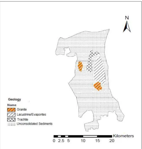
3.2.1.2 Geology of Kobo Valley

Figure 3.3 Geology of Kobo Valley (Source: Metaferia Engineering,2009)

3.2.2 General Hydrogeology

3.2.2.1 Hydrogeology of Ethiopia

Ethiopia has a complicated hydrogeological environment and complex groundwater regime. Until recently, many experts believed that extensive aquifers usable for large-scale exploitation of groundwater were unlikely to exist. This claim, which was almost a consensus, has recently been disputed due to a paradigm shift in methodology. There are indications that some aquifers in the count have large deposits of groundwater (Moges, 2012).

groundwater development. The Tertiary flood basalts can be major sources of groundwater, which under some circumstances are easy to tap (Ferriz and Bizuneh, 2003).

3.2.2.2 Hydrogeology of The Study Area

3.2.2.2.1 General

The valley and plain area are comprised of several low lying depositional areas distributed in the middle of the area extended from north to south. The mountain rises from 1500m to more than 2000 m and the plain is characterized by flat topography not greater than 1500m altitude. The plain area is formed by the accumulation of sediments from the surrounding scraps in an old lake bed. River drainage in the study area originates in from the western scraps where the youthful streams have cut deep gorges through the strata they cross and flow to the east across the plain to the Afar Depression through the narrow outlets in the eastern scraps. Due to low gradient, the streams form wide flood plain, alluvial flats and swamps as they reach the plain and deposit huge quantity of sediments. The soil type, as the geologic and hydrogeology report of the project, is dominantly alluvial sediment deposit from the escarpment of mountains. The soil is rich in organic and inorganic material for the production of crops (KGVDP feasibility report, volume II, Water Resource and Engineering, Regional Geology 1996).

3.2.2.2.2 Regional Setup

The regional hydrogological set up of the project area and its surrounding can be summarized as localized graben filling unconsolidated sediment composed of clay, silt, sand, gravel, boulders and pebbles above the Ashangi group volcanics which are intern underlain by Mesozoic sedimentary rocks.

3.2.2.2.3 Aquifer Thickness

The aquifer thickness varies over the valley. The thickness was determined from VES and drilling data.The material is considered as an aquifer if it is composed of layers of sand, gravel, pebbles and boulder. The lithological and electrical logs and the geophysical survey data of the sub surface material below the water table in each basin is analyzed to determine the thickness of the aquifer material. The sediment in Kobo-Arequaite-Gerbi sub-basin is mainly clay that less aquifer is expected. Water is hardly transmitted to wells at the required rate.

3.2.2.2.4 Aquifer Type

According to Metaferia Consulting Engineers report (2009), the groundwater aquifer type in the Kobo Valley development project is unconfined aquifer.

3.3 Climate and Rainfall

The principal feature of rainfall in the area is seasonal, poor distribution and variable from year to year. Rainfall distribution over the area is Bimodal, characterized by a short rainy season (Belg) and the long rainy season (Meher) that occurs in February-April and July-October respectively with a short dry spell from May to June (Feasibility Study Report for KGVDP, Volume II: Hydrology; CoSAERAR, 1999).

The position of Inter-Tropical Convergence Zone (ITCZ), seasonal variations in pressure systems and air circulation, results in the seasonal distribution of rainfall over the project area. This low pressure area of convergence between tropical easterlies and equatorial westerlies causes the equatorial disturbances to take place.

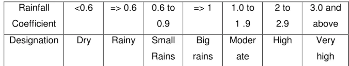
The distribution of rainfall over the highland areas is modified by orographic effects and is significantly correlated with altitude. Two rainy seasons have been experienced. The main rainy season often extends from end of June through end of September and the small rainy season from end of March to middle of April. The rest of the months are generally dry. The pattern of the seasonality of rainfall in the project area is determined by computing mean monthly rainfall ratio with that of rainfall module and compare with rainfall coefficient given by Gemechu classification as shown in the Table 3.1 below. The monthly rainfall of the study area for the concurrent selected 10 years is shown in Annex A.7.

Rainfall Coefficient

<0.6 => 0.6 0.6 to 0.9

=> 1 1.0 to 1 .9

2 to 2.9

3.0 and above Designation Dry Rainy Small

Rains

Big rains

Moder ate

High Very high

The mean annual rainfall of the watershed is estimated to be about 798.4 mm. As per Gemechu(1977)system of defining climatic or moisture regions, the basin is classified as dry sub-humid.

3.4 Drainage System

3.4.1 General

Kobo is a part of Kobo-Girana valley which comprises of Kobo, Girana and some part of the Raya valley. The major drainage system is associated with valley plains. The main river in the valley originates from the western mountains. The perennial rivers draining in to the valleys are the Hormat, Golina, Alawuha, Chereti and Gelana. There are also a number of intermittent streams which are draining westwards to the valley. The Kobo-Girana valley can be classified into seven major sub-basins and their respected locations are shwon in the Figure 3.4. These are the Waja-Golesha, Hormat-Golina, Kobo-Arequaite-Gerbi, Alawuha, Chireti, Gelana and the Hara sub-basins. Kobo Valley Development Project is a part of the first three sub basins, Waja-Golesha, Hormat-Golina and Kobo-Gerbi. The areal coverages of sub-basins in the Kobo-Girana valley are given in Table 3.2 below.

NAME AREA (km2) PERIMETER (km)

Hormat-Golina 794.95 122.95 Kobo-Gerbi 113.62 50.88 Waja-Golesha 556.30 113.63

Girana 450.86 90.07

Alawuha 661.84 127.30

Chereti 218.19 78.78

Hara 83.51 38.62

Table 3.2 Areal Coverages of Sub-Basins in Kobo Girana valley(Source:Metaferia Consulting Engineers,2009).

3.4.2 Waja Golesha Sub Basin

The Waja-Golesha sub-basin is drained by Gobu and Waja streams which disappear in Waja plain. There is one intermittent stream named Dikala stream which starts from the western ridge of Kobo Town and flows towards the Garalencha Mendefera before it disappears in the Chobe-Golesha plain.

3.4.3 The Kobo-Gerbi Closed Sub Basin

3.4.4 The Hormat Golina Sub Basin

The Hormat-Golina sub-basin constitutes the drainage systems of Hormat, Golina, Kelkeli and Weylet. Most of the flows of the rivers of this sub-basin too are lost in the plain before reaching their outlets through Golina River.

Hormat, Golina and Kelkeli are perennial rivers in general. However, during dry season, Hormat and Kelkeli lose their discharge in the plain before joining Golina that ultimately discharge through the Golina gorge to the Afar Depression. As it can be learnt from the aerial photo interpretation and from geophysical investigation, most of these rivers are fault and fracture controlled. In their upper course of the mountainous terrain, the slopes of these rivers vary from 4.2 to 6.9 %.

3.4.5 Groundwater Divide Line

The groundwater divide line helps to demarcate the extents of the sub basins in the study area. According to Metaferia Consulting Engineers (2009), the groundwater divide line is given in the Figure 3.5 below.

4. Data and Methodology

4.1 Data

In the study area there are around 100 water wells. Out of these 100 water wells 64 of them are currently functional and the study is based on these wells. In Ethiopia, controlling or monitoring the groundwater level is not done very well. Even if it is done, it is not really complete. An organized monitoring of groundwater was officially started in 2001 for few parts of the country. Kobo Girana Valley development project is one of the better monitored sites with regard to groundwater data in the country.

The main data required for this study are Geological data, Elevation of the study area, Hydro geochemical properties, aquifer thickness, sediment thickness, depth to groundwater table, and hydraulic permeability of the aquifers. The precipitation data for the Kobo area is obtained from National Meteorology Agency. The groundwater parameters are obtained from Ethiopian National Groundwater Database Association (ENGDA) under the Ministry of Water Resources. Some of the data are also obtained from Amhara Water Works Design and Supervision. The feasibility study of the Kobo Girana Valley Development Project is also a good source of data. The groundwater quality and aquifer data are shown in Annex 9 and 10 respectively. These data are collected until the year of 2009.

4.1.1 Data Preparation

Before the data are directly used for the intended purposes, they had to go through a certain procedures since they didn’t meet the requirements for ArcGIS software. The hardcopy of the maps (study area and others) had to be digitized and georeferenced. After the maps were georeferenced, they were converted to shapefiles so that ArcGIS can be effectively used. The projected coordinate system is UTM 37 N which represents the study area. The hydro geochemical and all aquifer parameters were made ready to be used in the Arc GIS software.

4.1.2 Data Cleaning

As Chapman (2005) said, error prevention is far superior to error detection and cleaning, as it is cheaper and more efficient to prevent errors than to try and find them and correct them later.

2005).Since we don’t have a huge data in this study, data cleaning softwareswere not used. The cleaning was done manually. The problems encountered are blank spaces, texts in numerical fields and big numbers. In general the data was not that noisy and it was easy to clean it.

4.1.3 Data transformation

Several methods in Geostatistical Analyst require that the data is normally distributed. When the data is skewed, it may be needed to transform the data to make it normal based on the aim we are achieving. In exploratory data analysis, the histogram and Normal QQ plot are used to explore the effect of different transformations. If the data is chosen to be transformed before creating a surface using geostatistics, the predictions will be transformed back to the original scale for the interpolated surface.

For Geostatistical analysis, based on the purpose we are thriving to achieve, data transformation or normalization may be needed. If we are just in need of surface predictions and map of prediction standard errors, the assumption of normal distribution of the data can be ignored on the classical kriging methods (ordinary, universal and Bayesian Kriging). On the other hand if the output surface is to generate quantile and probability maps, the assumption of normal distribution is necessary.

In this study, surface prediction is aimed; in order to produce the thematic maps and use them as an input for further investigations about the study area. Up on this aim (surface prediction), the assumption which uses normalization can be ignored since the classical methods of kriging don’t favour it.

4.1.4 Exploratory Data Analysis

Exploratory data analysis is the process of using graphs and other methods in order to look deep in to the data. It is useful to determine the different characteristics of the data into consideration. Before doing any geostatistical applications or predictions on the data, it is mandatory to do exploratory data analysis so that one can have a clear picture on the nature of the data and it compatibility for the intended purpose. Even the selection of the interpolation methods critically depends on the results of the exploratory analysis. In this study, the main exploratory analysis done includes statistics summary, histogram, Normal QQ plot, trend analysis and Voronoi. The exploratory analysis is done using both ArcGIS and Microsoft Excel.

4.1.4.1 Summary Statistics

measure of location or central tendency as a form of arithmetic mean, measure of statistical dispersion as standard deviation, a measure of the shape of the distribution like skewness or kurtosis and if more than one variable is measured a measure of statistical dependence such as correlation coefficient.

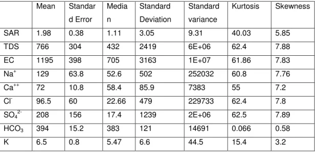
Mean Standar d Error Media n Standard Deviation Standard variance

Kurtosis Skewness

SAR 1.98 0.38 1.11 3.05 9.31 40.03 5.85 TDS 766 304 432 2419 6E+06 62.4 7.88 EC 1195 398 705 3163 1E+07 61.86 7.83 Na+ 129 63.8 52.6 502 252032 60.8 7.76 Ca++ 72 10.8 58.4 85.9 7383 55 7.2 Cl- _{96.5 60 22.66 479 229733 62.4 7.8}

SO42- 208 156 17.4 1239 2E+06 62.5 7.89

HCO3 394 15.2 383 121 14691 0.066 0.58

K 6.5 0.8 5.47 6.6 44.5 15.4 3.2

Table 4.1 Descriptive Statistics of groundwater parameters

The Table 4.1 shows the descriptive statistics of the nine groundwater parameters selected for this study. The summary includes the mean, standard error, median, standard deviation, variance, kurtosis and skewness.

The mean is influenced by the big number that is registered in the well TK3 which is an outlier. The standard error is also big except for SAR and Hydraulic Conductivity (K). Except for Sodium Adsorption Ratio (SAR) and Hydraulic Conductivity, all the other parameters have huge values for standard deviation and variance. Apart from this all parameters have a kurtosis value greater than 40 except from hydraulic conductivity and bicarbonate which has 15.4 and 0.066 respectively. In general, the kurtosis value is very big for the distribution to be normal.

Table 4.2 Correlation coefficient values of the groundwater quality parameters

The table above shows the correlation coefficient among the hydro geochemical parameters of the groundwater. It can be seen that the Sodium Adsorption Ratio (SAR) has almost a perfect correlation with TDS, Ec, Na, Ca, Mg, Cl and SO4. The correlation coefficient ranges from 86.7 to 93.3%. On the contrary, SAR has very small correlation with bicarbonate (HCO3) with a value of 6.5%.

Total Dissolved Solids (TDS) has a perfect correlation with Ec, Na+_{, Ca}++_{, Cl}- _{and SO}

42-. The

correlation ranges between 97.4 to 99.9 %. Similar to SAR, TDS has a very small correlation which is -5.6%. The negative sign shows that this very small correlation is negative.

In general, it can be seen that bicarbonate (HCO3-) has very small correlation with the other

groundwater chemical parameters.

4.1.4. 2 Histograms

Histogram is used to graphically show how the univariate data is distributed. A histogram is probably the most commonly used way of displaying data. Simply stated, a histogram is a bar chart with the height of the “bars” representing the frequency of each class after the data have been grouped into classes. The histogram graphically shows the centre of the data, the spread of the data, skewness of the data, presence of outlier and presence of multiple mode in the data. These features provide strong indications of the proper distributional model for the data.

In this study, Histograms are made for individual groundwater quality parameters like TDS, EC, SAR, Na, Ca, SO4, HCO3 and Cl using ArcMap software. Besides to these groundwater quality parameters, histogram is constructed for hydraulic conductivity or permeability of the aquifer. The figure showing the histogram for all parameters is given in Annex A.1.

It has been observed that, the values at bore hole TK3 are located at the extreme end of the histogram leaving other values to the left. This is an indication that the values recorded at the TK3 might be an error in the reading or just an extreme value. This might suggest that we have an outlier in the data. Apart from this, the skewness values are more than 1 or -1 in almost all of the histograms and this is an indication of the lack of normal distribution due to the presence of extreme values at well TK3. When the values at TK3 are removed, the histograms show normal distribution pattern than the previous.

When the extreme value at well TK3 is removed, the histogram shows a bell like structure on the plot for most of the groundwater parameters which is an indication of normal distribution of the data.

4.1.4.3 Normal QQ Plot

Normal QQ plot is done to asses if the data samples are whether normally distributed or not. If the data points fall on the line of the Normal QQ plot, it can be said that the data in consideration is normally distributed. Otherwise, it is not normally distributed.

For the groundwater parameters in this study, as shown in Annex II, the data points don’t fall on the straight line on the Normal QQ plot. This implies that the parameters in question are not normally distributed. This may be due to the extreme big values at well TK3. This fact is also shown in the Histogram and summary statistics analysis. Once the Outlier or extreme value is removed, most of the data points fall on the straight line of the Normal QQ plot. The Normal QQ plot for the groundwater parameters is shown in Annex A.2.

4.1.4.4 Trend Analysis