Array-database Model (SciDB) for Standardized Storing of Hyperspectral Satellite Images
Texto
Imagem
![Figure 1 Electromagnetic Spectrum [Shippert 2003].](https://thumb-eu.123doks.com/thumbv2/123dok_br/15759853.639448/17.893.162.763.636.797/figure-electromagnetic-spectrum-shippert.webp)
![Table 1 Hyperspectral Sensors and Data Providers [Shippert 2003].](https://thumb-eu.123doks.com/thumbv2/123dok_br/15759853.639448/18.893.140.777.400.1117/table-hyperspectral-sensors-data-providers-shippert.webp)
![Figure 2 Evolution of remote sensing spectroscopy with respect to spectral resolution [Belokon 1997]](https://thumb-eu.123doks.com/thumbv2/123dok_br/15759853.639448/20.893.254.661.124.669/figure-evolution-sensing-spectroscopy-respect-spectral-resolution-belokon.webp)
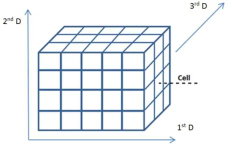
![Figure 3 Hyperspectral Cube [Manolakis and Shaw 2002].](https://thumb-eu.123doks.com/thumbv2/123dok_br/15759853.639448/21.893.157.763.127.573/figure-hyperspectral-cube-manolakis-shaw.webp)
![Figure 4 Energy Reflectance of the Electromagnetic Spectrum [Smith 2006].](https://thumb-eu.123doks.com/thumbv2/123dok_br/15759853.639448/23.893.172.744.135.518/figure-energy-reflectance-electromagnetic-spectrum-smith.webp)
![Figure 5 Reflectance Spectrum for different surfaces [Shippert 2003].](https://thumb-eu.123doks.com/thumbv2/123dok_br/15759853.639448/24.893.186.759.144.439/figure-reflectance-spectrum-different-surfaces-shippert.webp)

Documentos relacionados
In this dissertation, our purpose is to build different ensemble methods to compare and to analyse the results of accuracy obtained (on their classification of satellite images
Using the satellite CBERS2B/CCD, images were used to identify and quantify irrigated areas and then associate these areas with a database containing
Using a free software for satellite image analysis, the photointerpretation showed that the NS, NE and NW directions observed on the Pantanal satellite images are the same recorded
Comparing the results of hyperspectral imagery classification with the optimized classification system of hybrid images show that using DSM beside hyperspectral imagery
So we introduce the Correctness Coefficient (CC) method. Also, several procedures for subpixel accuracy assessment were introduced. The numbers of binary images are
The analysis of the dynamics of chotts and sabkhas based on medium resolution satellite images on two different dates (Landsat TM 1987 and TM 2009) specializes (mapping)
In this work, we carried out feature extraction using modified view based approach of original and thinned images and sub images of original and thinned images for
Mennis (2003) used the combination of dasymetric mapping, advanced three-class method and empirical sampling based on satellite images to model the population distribution
