Ocean Sci., 9, 477–487, 2013 www.ocean-sci.net/9/477/2013/ doi:10.5194/os-9-477-2013
© Author(s) 2013. CC Attribution 3.0 License.
Geoscientiic
Geoscientiic
Geoscientiic
Ocean Science
Open Access
MERIS-based ocean colour classification with the discrete
Forel–Ule scale
M. R. Wernand1, A. Hommersom2, and H. J. van der Woerd2
1Royal Netherlands Institute for Sea Research, Physical Oceanography, Marine Optics and Remote Sensing, P.O. Box 59,
1790AB Den Burg, Texel, the Netherlands
2Institute for Environmental Studies (IVM), VU University Amsterdam, De Boelelaan 1087, 1081 HV Amsterdam,
the Netherlands
Correspondence to:M. Wernand ([email protected])
Received: 13 July 2012 – Published in Ocean Sci. Discuss.: 31 August 2012 Revised: 27 March 2013 – Accepted: 11 April 2013 – Published: 2 May 2013
Abstract. Multispectral information from satellite borne ocean colour sensors is at present used to characterize nat-ural waters via the retrieval of concentrations of the three dominant optical constituents; pigments of phytoplankton, non-algal particles and coloured dissolved organic matter. A limitation of this approach is that accurate retrieval of these constituents requires detailed local knowledge of the specific absorption and scattering properties. In addition, the retrieval algorithms generally use only a limited part of the collected spectral information. In this paper we present an additional new algorithm that has the merit of using the full spectral in-formation in the visible domain to characterize natural waters in a simple and globally valid way. This Forel–Ule MERIS (FUME) algorithm converts the normalized multiband re-flectance information into a discrete set of numbers using uniform colourimetric functions. The Forel–Ule (FU) scale is a sea colour comparator scale that has been developed to cover all possible natural sea colours, ranging from in-digo blue (the open ocean) to brownish-green (coastal water) and even brown (humic-acid dominated) waters. Data using this scale have been collected since the late nineteenth cen-tury, and therefore, this algorithm creates the possibility to compare historic ocean colour data with present-day satel-lite ocean colour observations. The FUME algorithm was tested by transforming a number of MERIS satellite images into Forel–Ule colour index images and comparing in situ observedFUnumbers withFU numbers modelled from in situ radiometer measurements. Similar patterns andFU num-bers were observed when comparing MERIS ocean colour distribution maps with ground truth Forel–Ule observations.
TheFUnumbers modelled from in situ radiometer measure-ments showed a good correlation with observedFUnumbers (R2=0.81 when full spectra are used andR2=0.71 when MERIS bands are used).
1 Introduction
The application of optical satellite remote sensing tech-niques to monitor the radiation scattered back from the water column became a major breakthrough in the seven-ties for monitoring ocean, sea and coastal areas (IOCCG, 1998). Dedicated ocean colour instruments, like CZCS, Sea-WiFS, MERIS and MODIS-AQUA, have provided funda-mental new insights into the dynamics and role of oceanic plankton (e.g. Behrenfeld et al., 2006). Observations are now starting to span multiple decades, allowing a first glimpse at long-term variations in the plankton composition of the oceans, which are potentially related to global change (An-toine et al., 2005; Polovina et al., 2008).
local water constituents, or complex, with a need for detailed measurements of the specific absorption and scattering prop-erties of these in-water constituents (see, e.g. Tilstone et al., 2012). The derived water-quality parameters are the major products of ocean colour instruments, while the colour itself can be considered as a primary product.
Long before the development of diode arrays to measure spectral radiation, another method had been developed and tested which recorded the colour of natural waters. Towards the end of the nineteenth century, Forel and Ule (Forel, 1890; Ule 1892) proposed a method to classify the colour of the oceans, regional seas and coastal waters using a colour com-parator scale. The scale became known as the Forel–Ule (FU) scale and since then scale observations have been per-formed, generating hundreds of thousands of data points at global scale for more than a century. Recently, it was shown (Wernand and Van der Woerd, 2010a) that theFUscale can be used to characterize the colour of natural waters. More im-portantly, the analysis ofFUcolour variation in the North Pa-cific since 1930 has revealed significant variations at decadal timescales (Wernand and Van der Woerd, 2010b).
In this paper we describe a simple algorithm to couple his-torically collected ocean colour data, obtained over a long time span, with presently available satellite-derived ocean colour imagery for hindcasting long-term changes. This Forel–Ule to MERIS (FUME) algorithm converts MERIS observations of sea- and ocean colour to chromaticity co-ordinates and subsequently to a discrete Forel–Ule number. This will result in a new MERIS water quality product that can be used as a simple and straight-forward index of wa-ter colour in addition to the wawa-ter-quality paramewa-ters that are retrieved by inversion schemes. Based on the FUME prod-uct, ocean colour trends can be constructed, reaching back to over one hundred years. Distinct optical water types can now be classified according to the Forel–Ule scale and this makes it possible to enhance satellite derived products, such as chlorophyll (Moore et al., 2009). Ocean colour remote sensing techniques have traditionally been based on two opti-cal water types, known as “Case 1” and “Case 2” (Morel and Prieur, 1977). However, this classification is mainly based on the intrinsic composition, i.e. the role of algae (and related degradation products) in the generation of water colour.
Moore et al. (2009) proposed extending the optical wa-ter classification to eight cluswa-ters, based on an unsupervised classification of the NOMAD database of remote sensing re-flectance spectra. The reflection spectrum of each satellite pixel has a certain probability of belonging to each of the 8 clusters. Another classification method that can be tuned to local properties is proposed by Hommersom et al. (2011). In this work we go back to use the oldest classification of 21 pre-defined scales and use the relative colour difference (colour comparator scale) instead of absolute remote sensing reflectance to classify each pixel to only one representative FUnumber.
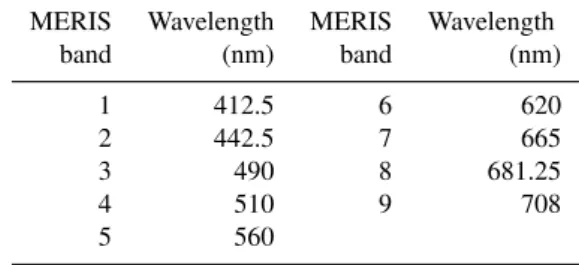
Table 1. Central wavelengths of the first nine MERIS spectral bands. All bands have a width of 10 nm, with the exception of band 8 (7.5 nm).
MERIS Wavelength MERIS Wavelength band (nm) band (nm)
1 412.5 6 620
2 442.5 7 665
3 490 8 681.25
4 510 9 708
5 560
2 Methods
In this section we introduce the MERIS satellite data, the algorithm to convert MERIS reflection data toFUnumbers and the ship-borne measurements for a first characterization of the FUME results.
2.1 MERIS products
MERIS is a 68.5◦field-of-view push-broom imaging spec-trometer (Rast et al., 1999) on the ENVISAT platform. It measures the solar radiation reflected by the ocean at a spatial resolution of 260 m×290 m in 15 spectral bands. The bands are programmable in width and position, at visible and near-infrared (NIR) wavelengths. MERIS provides global cover-age in 3 days with radiation reflected by the ocean that is atmospherically corrected to derive the normalized water-leaving reflectances, a MERIS Level 2 product (ESA, 2012). The atmospheric correction assumes that the water totally absorbs the NIR, but also includes a correction for those sediment loaded waters where this assumption fails. Nor-malized water-leaving reflectance (dimensionless) [ρW]N is
defined by Eq. (1) as follows: [ρW]N(λ)=
[LW]N(λ)
F0(λ)
, (1)
where [LW]Nis the normalized water-leaving radiance
(Gor-don and Voss, 1999) and F0 is the extraterrestrial solar
ir-radiance at wavelength (λ). In this analysis, data is lim-ited to the visible spectrum, covering the first nine MERIS bands with bandwidths of 10 nm, except for band 8 which has a bandwidth of 7.5 nm (Table 1). In the standard pro-cessing by ESA, a number of global products are derived together with [ρW]Nthat will be used to compareFU
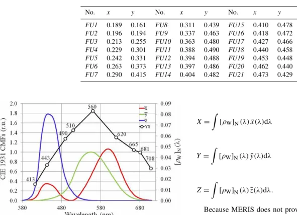
Table 2.Chromaticity coordinates (x,y) of theFUscale numbers as determined by Wernand and Van der Woerd (2010a).
No. x y No. x y No. x y
FU1 0.189 0.161 FU8 0.311 0.439 FU15 0.410 0.478 FU2 0.196 0.194 FU9 0.337 0.463 FU16 0.418 0.472 FU3 0.213 0.255 FU10 0.363 0.480 FU17 0.427 0.466 FU4 0.229 0.301 FU11 0.388 0.490 FU18 0.440 0.458 FU5 0.242 0.331 FU12 0.394 0.488 FU19 0.453 0.448 FU6 0.263 0.373 FU13 0.397 0.486 FU20 0.462 0.440 FU7 0.290 0.415 FU14 0.404 0.482 FU21 0.473 0.429
Fig. 1.The CIE 1931 2◦Colour Matching Functions forx¯ (red),
¯
y(green) andz¯ (blue) determined per nanometre. The black line shows a reconstructed spectrum (Yellow Sea) of MERIS reflectance measured at nine bands (open circles).
2.2 The FUME algorithm
The FUME algorithm converts the normalized water-leaving reflectance from nine MERIS bands into a discrete FU number in three steps. Step 1: calculation of the tristim-ulus values X, Y, Z by calculating the convolution of the colour-matching functions (CMFs) and the normalized water-leaving reflectance (CIE, 1932). Step 2: calculation of the (x,y)chromaticity coordinates by the ratio ofXorY tris-timulus values and the sum of the tristris-timulus values. Step 3: determination of theFUscale number by comparison of cal-culated (x,y) values to the unique chromaticity coordinates of the twenty-oneFUnumbers.
Step 1: tristimulus values are the amounts of three pri-maries that specify a colour stimulus of the human eye (Wyszecky and Stilles, 2000) and are noted asX,Y andZ
(CIE, 1932). The CIE 1931 standard colourimetric 2-degree CMFsx¯(red),y¯(green) andz¯(blue) are presented in Fig. 1. These serve as weighting functions for the determination of the tristimulus values of the MERIS normalized water-leaving reflectance [ρW]Nby Eq. (2a), (b) and (c):
X= Z
[ρW]N(λ)x(λ)¯ dλ (2a)
Y = Z
[ρW]N(λ)y(λ)¯ dλ (2b)
Z= Z
[ρW]N(λ)z(λ)¯ dλ. (2c)
Because MERIS does not provide full-spectral coverage, the reflection spectrum is first reconstructed by linear in-terpolation between bandn=1 (412.5 nm) and bandn=9 (708 nm) with a resolution of 1 nm. An example is shown as a black line in Fig. 1. Note that the linear interpolation atλi (nm) is always carried out between subsequent bands (n,n+1) with the condition (λn< λi< λn+1). The
tristim-ulus values forX,Y andZare obtained by a Riemann sum approximation of the integrals with1λ=1 nm resolution:
X=X708
i=413[ρW]N(λi) x(λ)1λ (3a)
Y =X708
i=413[ρW]N(λi) y(λ)1λ (3b)
Z=X708
i=413[ρW]N(λi) z(λ)1λ. (3c)
Step 2: subsequently, the chromaticity coordinatesx,yand
zare calculated from the ratio of each of the tristimulus val-ues and the sum of the valval-ues:
x= X
X+Y+Z y= Y
X+Y+Z z= Z
X+Y+Z. (4)
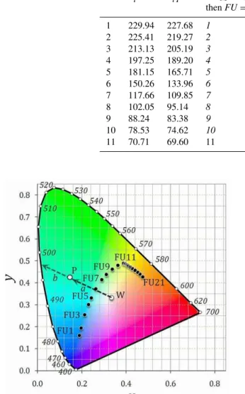
Table 3.AnglesαiofFUnumber in degrees (i=1 to 21) and the 20 boundary anglesαiT that are used in the discrete classification of ocean
colour.
i αi◦ αiT◦ IfαM> αiT i α◦i α
◦
iT IfαM> αiT
thenFU= thenFU=
1 229.94 227.68 1 12 68.49 67.93 12 2 225.41 219.27 2 13 67.36 65.98 13 3 213.13 205.19 3 14 64.60 63.35 14 4 197.25 189.20 4 15 62.11 60.37 15 5 181.15 165.71 5 16 58.62 56.64 16 6 150.26 133.96 6 17 54.65 52.09 17 7 117.66 109.85 7 18 49.53 46.75 18 8 102.05 95.14 8 19 43.96 41.82 19 9 88.24 83.38 9 20 39.67 36.98 20 10 78.53 74.62 10 21 34.28 21 11 70.71 69.60 11
Fig. 2.The chromaticity coordinates, based upon transmission mea-surements, of theFUscale colours 1 to 21 (black circles) and the white pointW(wherexW=yW=1/3). The outer curved boundary
is the spectral locus, with the corresponding monochromatic wave-lengths shown in nanometres.
between W and an arbitrary point P (a) and the distance fromW to the spectral locus (a+b), gives the colour sat-uration (a/(a+b))or the intensity of the colour atP. In this way, the chromaticity coordinates (xM, yM)for every MERIS
pixel can be calculated.
Step 3: in the next step the (xM, yM)is converted to aFU
number. The originalFUscale was created to make an ob-jective classification of natural waters (see for a review Wer-nand and Gieskes, 2011). In 21 glass tubes a variable mixture of three standard solutions (distilled water, ammonia, cop-per sulphate, potassium chromate and cobalt sulphate) were created to obtain the colour palettes of the scale. These
stan-Fig. 3. Chromaticity diagram with scale colours FU1 to FU21 shown as dots, relative to the white point that is set at the origin. As an example the angleαi(102.05◦, see Table 3), determining the
position ofFU8, is given.
dard solutions were recently reconstructed and their optical properties were measured in the laboratory with medium res-olution spectrometers (Wernand and Van der Woerd, 2010a). The calculated chromaticity coordinates of the originalFU scale are presented in Table 2 and graphically shown as a line of black dots, between the white point and the locus, in the chromaticity diagram of Fig. 2. The FUME algorithm first shifts the origin to the white pointW with chromaticity coordinatesxW=yW=1/3 (Fig. 3). Then it calculates the
angle (αM)between the vector to a point with certainFU
co-ordinates (xM,yM)and the positivex-axis (aty−yW=0),
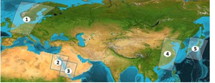
Fig. 4. Areas where MERIS data were extracted from ESA’s MERCI database.
Fig. 5.Left: MERIS true colour image (4 May 2006). Right: the springFUmap of the turbid North Sea showsFUvalues ranging from 3 to 9 (red circle near EnglandFU6). The Wadden Sea area within barrier islands north of Holland shows values betweenFU9 andFU18. The area within the red circle indicates a pixel value ofFU=14. The yellow line shows the transect extracted from the MERIS image and shown in Fig. 9.
All calculations were made with the atan2 function (four-quadrant inverse tangent) and the derived angles (in radians) were multiplied by 180/πto get the angles in degrees:
αM=arctan(yM−yWxM−xW)modulus 2π. (5)
Two examples are shown in Fig. 3.αi is the angle match-ing FU8. The yellow dot is derived from the normalized spectral reflectance of a MERIS-pixel and coordinates (xM−
xW= −0.15, yM−yW=0.1) and angle (αM). Finally, the
boundaries distinguishing the variousFUnumbers were de-fined. The colour transition angleαiT, under which a scale number transition takes place, was taken according to Eq. (6):
αiT =
(αi+αi+1)
2 . (6)
BothαiandαiT are presented in Table 3. TheFUnumbers for a given MERIS pixel M with chromaticity coordinates
xM–xW= −0.15 andyM–yW=0.1 (yellow point in Fig. 3)
can be determined as follows: first the angle (Eq. 5) is de-termined asαM=146◦and then is compared with a simple
MATLAB loop fori=1 to 21 values ofαiT given in Table 3. From this loopαM> αiT is true for the first time reaching the
Fig. 6. The winterFU map of the Red Sea, dated 22 (left) and 23 December 2003 (right) shows that open water of the northern part is mainly bluish FU1toFU2(in red circle FU2), and near coast values are aroundFU3. The southern part shows more green-ish coloured water (in red circleFU=8).
Fig. 7.The winter FU map of the Yellow Sea, acquisition date 11 February 2009 (left), and the summerFU map of the Sea of Japan, acquisition date 14 June 2004 (right). The Yellow Sea is mainly greenish brown withFU7up toFU17(FU9in the lower red circle andFU11in the upper red circle). The Sea of Japan, a “blue sea”, shows summer values of aroundFU2to FU3(in red circleFU2). East of Hokkaido phytoplankton abundance greens the water toFU10(FU9within the red circle to the east).
angleαiT =133.96 degrees, which corresponds to a discrete value ofFU=6 that is attributed to this MERIS pixel M. 2.3 Ship-borne measurements
The North Sea and the Wadden Sea (Hommersom et al., 2009) were optically sampled in 2006 (Fig. 5) and several lakes and rivers were sampled in 2001, 2006 and 2007. The surface radiance Lsfc, sky radiance Lsky and
incom-ing solar irradiance Es were measured simultaneously,
Fig. 8.Example of the pixel values of MERIS normalized water-leaving reflectance spectra of the North Sea (NS), Wadden Sea (WS), Yellow Sea (YS), Sea of Japan (SJP) and the northern and southern Red Sea (RS1 and RS2, respectively). Notice the similar-ity in the spectral shapes of the Wadden Sea spectra; WS is a MERIS normalized water-leaving reflectance spectrum and WS (GT) is the ground truth reflectance spectrum from ship-based measurements.
1999). Remote sensing reflectance was then calculated as
RRS=Lw/Es, where Lw is the water-leaving radiance (=
Lsfc−ρLsky)andEsis the downward irradiance just above
the sea surface (Mueller et al., 2003). To a good approxima-tion, [ρW]N≈π RRS(Lee et al., 1994).
To illustrate the potential use of the satellite derivedFU maps, databases containing globally collected ship-borneFU observations were consulted. From the oceanographic and meteorological database, archived by the United States Na-tional Oceanographic Data Centre (NOAA-NODC; Boyer et al., 2006), and from the ocean colour database at the Royal Netherlands Institute for Sea Research, FU observations were extracted. To create the maps,FUmeasurements were interpolated through an inverse distance weighted (IDW) technique (Watson and Philip, 1985) in an ARCGIS environ-ment. The IDW interpolation was carried out over 2 degrees with a grid size of 0.2◦.
3 Datasets
The FUME algorithm was applied to five MERIS images acquired over the areas shown in Fig. 4. These areas were chosen for their different sea colour properties (Wernand et al., 2013) and cover the North Sea (1), the Red Sea (2, 3), the Yellow Sea (4) and the Sea of Japan (5). The im-ages were extracted from ESA’s online database, the MERIS Catalogue and Inventory (MERCI, Brockman et al., 2005). MERIS Reduced Resolution (RR) geophysical products (Ta-ble 4) contain, among other products, a total of 14 spec-tral images of normalized band reflectances and the derived products for pigments (Algal-1, Algal-2, SPM and YS). A Reduced Resolution image has 4×4 less pixels than the
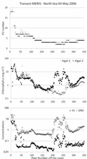
Fig. 9.Transect from the inner Wadden Sea to the central North Sea. The upper panel shows theFUvalues, the middle panel shows the two MERIS products for chlorophylla, and the lower panel shows the concentration of SPM (units in g m−3)and yellow substance (absorption in m−1at 442 nm).
same image in Full-Resolution, thus representing an area of 1040 m×1160 m.
To validate the FUME algorithm, a dataset of 53 simul-taneously collectedFUobservations and hyperspectral sub-surface and above-water spectra was consulted. This dataset was established in 2001 and contains observations and op-tical data of a wide range of coloured water types, such as river, lake, coastal and open sea, with the FU scale vary-ing fromFU3 (open sea) toFU21(lakes). In addition, one dataset was included from Hommersom et al. (2009) that was made close (2.5 h prior) to the MERIS image acquisition time on 4 May 2006.
Table 4.Reference to the acquired MERIS Reduced Resolution images.
Sea Area Product name Start time UTC
North Sea 1 MER RR 2PQBCM20060504 04-MAY-2006 10:11:24 Red Sea north 2 MER RR 2PQBCM20031222 22-DEC-2003 07:56:09 Red Sea south 3 MER RR 2PQBCM20031223 23-DEC-2003 07:26:02 Yellow Sea 4 MER RR 2PPBCM20090211 11-FEB-2009 02:27:39 Sea of Japan 5 MER RR 2PQBCM20040614 14-JUN-2004 01:07:24
Table 5.RGB values for the reproduction of theFUlegend.
FUno. R G B FUno. R G B
1 33 88 188 12 148 182 96 2 49 109 197 13 165 188 118 3 50 124 187 14 170 184 109 4 75 128 160 15 173 181 95 5 86 143 150 16 168 169 101 6 109 146 152 17 174 159 92 7 105 140 134 18 179 160 83 8 117 158 114 19 175 138 68 9 123 166 84 20 164 105 5 10 125 174 56 21 161 77 4 11 149 182 69
has not yet been recorded in the central archives. Therefore, we have chosen to show data from the same seasons in ear-lier years. For the Red Sea, 52 observations are available and were collected during the winters of 1895 to 1898. For the Yellow Sea, 2882FUobservations were collected during the winters of 1930 to 1999.
4 Results
4.1 MERISFUmaps
For all five MERIS images the reflectance values in bands 1– 9 per pixel were converted to chromaticity coordinates and intoFUnumbers using Eqs. (3) to (5). Converted images are further referred to asFUmaps. TheseFUmaps are presented in Figs. 5, 6 and 7. In these figures we have used the MERIS flags per pixel to identify land (grey), clouds (white) and the failure to collect observations or retrieve water-leaving re-flectances (black). The legend (RGB – red, green, blue – val-ues are given in Table 5) represents theFUcolours as close as possible. The [ρW]N spectral signatures at the locations
marked with a red circle in the maps are plotted in Fig. 8. The first FU map shown in Fig. 5, acquisition date of 4 May 2006, covers the North Sea, the Baltic and the Wadden Sea. The colour of the North Sea varies betweenFU3 and FU9. The colour within the left red circle situated between the Thames and Humber estuaries was estimated asFU6. The central North Sea shows values ofFU3toFU4with an
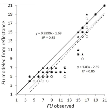
oc-Fig. 10a.Scatter plot of theFUnumbers modelled using full re-flectance spectra (black triangles) with trend line (dotted), and from the reflectance of MERIS bands (open circles) with trend line (in-termittent), versus in situ observedFUnumbers. The full black line is the 1:1 line. See Fig. 10b for the confusion matrix.
casionalFU2(very blue oceanic waters). The Wadden Sea, a large intertidal sea behind multiple barrier islands, north of Holland and Germany and west of Denmark, is dominated by sediment and outflow of humic-acid rich river water and has higherFUvalues, up toFU=18.
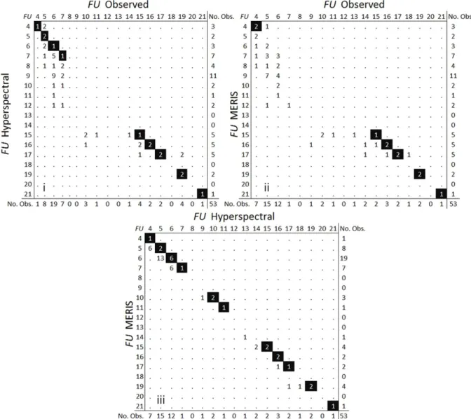
Fig. 10b.The confusion matrices of (i)FUmodelled hyperspectral data as a function of observedFUnumber, (ii)FUmodelled MERIS data as a function of observedFUnumber, and (iii)FUmodelled from MERIS spectral bands as a function ofFUmodelled hyperspectral data.
Figure 7 showsFU maps of the Yellow Sea (left) and the Sea of Japan (right) acquired on 11 February 2009 and 14 June 2004, respectively. The outflow of the Yangtze River (south of the red circle in the left image) shows highFU val-ues, betweenFU7up to real brownish colours ofFU19. Un-fortunately, the area close to the river outflow is flagged as a “no data area”. Within the red circle a value of FU9 is calculated. The Sea of Japan (right panel) shows values of FU2 toFU3 (within the red circle the value is FU2). Re-markable is the relative green area east of Hokkaido (FU9 marked by the red circle east) with values up toFU10. To verify our results the MERIS Level 2 chlorophyll product was consulted, which showed high concentrations of chloro-phylla (>2 mg m−3)east of Hokkaido and concentrations
between 0.1 and 0.5 mg m−3in the Sea of Japan.
4.2 Ground truth
The reflection spectrum at the match-up station in the Wad-den Sea (WS (GT)) is plotted in Fig. 8 and appears very sim-ilar in shape to the MERIS spectrum (WS). By extraction of the reflection at exactly all 9 MERIS bands and running the FUME algorithm, a value ofFU=15 was retrieved. The MERIS pixel at this location (red circle in the Wadden Sea) has a calculatedFUvalue of 14, which is in good agreement with the ground truth FU value considering possible adja-cency effects of tidal flats within the pixel.
Fig. 11.The Red Sea map based on 52FUin situ observations collected during the winters of 1895 to 1898. Within the northern red circle FU=2 and within the southern red circleFU=7. This colour boundary can also be observed 100 yr later in the MERIS map of Fig. 6.
Fig. 9. Within the first 30 pixels the waters are within or close to the Wadden Sea, characterized by very high loads of sedi-ment (>1 g m−3)and yellow substance (absorption>1 m−1
at 442 nm), corresponding toFUvalues above 7. In the next part (pixels 30–170), theFU values show a gradual gradi-ent from 7 to 3, reflecting a decrease in algal pigmgradi-ents (both Algal-1 and Algal-2 products) because both YS and SPM are rather constant in this interval. An interesting feature can be observed in the pixels (170–300) where the Case 2 wa-ter algorithm seems to fail (unrealistic high SPM and YS), likely due to additional scatter by cirrus clouds. Fortunately, theFUscale seems robust and corresponds rather well with the Algal-1 product.
Based on field measurements, a comparison between ob-served and modelledFUnumbers was made (Fig. 10). The correlation between observed and modelledFU numbers is around the 1:1 line (black line, Fig. 10a). To give additional insight into the results presented in Fig. 10a, confusion ma-trices were made from the rather sparse data and are pre-sented in Fig. 10b. For modelled hyperspectral data as a func-tion of observedFU(Fig. 10b-i), 51 % is within 1FUscale number; for modelled MERIS data as a function of observed FU(Fig. 10b-ii), 40 % is within 1FUscale number; and for the modelled MERIS data as a function of modelled hyper-spectral data (Fig. 10b-iii), 98 % is within 1FUscale num-ber.FUnumbers derived from the full spectrum and MERIS derivedFUcorrelate equally with in situ data (R2=0.85). The largest outliers were found in the 11–16FUmid-range. These are the green-yellowish water colours, which corre-sponds to∼500–600 nm visible light. The 11–16FUcolours are very close in the chromaticity diagram; therefore, small errors in the modelledFUcould induce a wrongFUindex. This problem may explain part of the outliers of Fig. 10a.
Comparing the MERIS winterFU maps of the northern and southern Red Sea in Fig. 6 with the winter IDW FU map of Fig. 11, similar patterns can be recognized despite a time gap of over a century between data acquisition. When we compare these maps, it seems that the colour of the Red Sea did not change significantly over time, although we can-not say anything about intermediate colour changes between 1899 and 2002. Within the red circles, the MERISFUmap (Fig. 6) showsFU2 for the northern location and FU8 for the southern location, while the IDWFUmap gives identical values at both locations.
TheFUmap for the Yellow Sea, based on 2882FUin situ observations collected during the winters of 1930 to 1999, is shown in Fig. 12. The Yellow Sea showsFUnumbers ofFU4 in open sea areas to values ofFU20in front of the outflow of the Yangtze River. Both the MERIS map of Fig. 7 and the IDW interpolation of Fig. 12 show similar colour patterns. The red circles on the MERIS map indicateFU9in the lower andFU11in the upper. In the IDW map, respectively,FU12 andFU14are indicated. A possible explanation of the bluing of the water (bluer colours show up in the 2008/9 map) is the reduced outflow of Yangtze water into the Yellow Sea
due to the hydroelectric Three Gorges Dam which became operational in 2003. The effect is a reduced upwelling and thus productivity, resulting in less green water (Chen, 2000; Gong et al., 2006).
5 Discussion and conclusions
In this paper an algorithm is presented that allows retrieval of the Forel–Ule sea colour from the MERIS satellite sen-sor. The Forel–Ule colour can be seen as the colour standard closest to the real colour of water. The elegance of our al-gorithm is that it converts multispectral observations to one simple number that is only dependent on a well-known uni-versal set of colourimetric functions. The classification of sea water is simplified by means of a numerical value between 1 and 21, instead of a classification by a normalized water-leaving spectral reflectance signature or the concentrations of the dominant optical constituents.
The approach is demonstrated by the processing of multi-spectral observations of oceans and coastal waters made by the MERIS ocean colour sensor toFUmaps that cover colour classes between indigo blue, green and brown. Five differ-ent seas were selected worldwide; these were processed to obtainFUmaps. The maps show very detailed patterns and gradients, mainly in the near coastal zones as expected by the more pronounced hydrographical gradients there. When the MERIS maps of sea and ocean colour distribution were com-pared with ground truth Forel–Ule observations mapped in the same season, similar patterns andFUnumbers were ob-served, even whenFUnumbers of more than a century ago were processed. This opens new ways to study the spatial and temporal evolution of the colour of the sea worldwide. The FUME algorithm can easily be adapted to data from other satellites that have enough bands in the visible part of the spectrum to properly derive the colour of the water.
Acknowledgements. Marieke Eleveld, Steef Peters and Reinold Pasterkamp from the Institute for Environmental Studies, Free University, Amsterdam, are thanked for their initiative to develop MATLAB routines that were used and adapted to generate satellite derived Forel–Ule maps. Menno Regeling is thanked for the Forel– Ule data collection in the North Sea (June 2001). Thanks are due to W. Gieskes (Dept. Ocean Ecosystems, University of Groningen, the Netherlands) for discussions and comments. MERIS data has been provided by the European Space Agency (ESA). We would like to thank J. Piera Fernandez for his suggestions to improve Fig. 3 and Fig. 10.
References
Antoine, D., Morel, A., Gordon, H. R., Banzon, V. F., and Evans, R. H.: Bridging ocean colour observations of the 1980s and 2000s in search of long-term trends, J. Geophys. Res. 110, C06009, doi:10.1029/2004JC002620, 2005.
Behrenfeld, M. J., O’Malley, R. T., Siegel, D. A., McClain, C. R., Sarmiento, J. L., Feldman, G. C., Milligan, A. J., Falkowski, P. G., Letelier, R. M., and Boss, E. S.: Climate-driven trends in con-temporary ocean productivity, Nature, 444, 752–755, 2006. Boyer, T. P., Antonov, J. I., Garcia, H. E., Johnson, D. R., Locarnini,
R. A., Mishonov, A. V., Pitcher, M. T., Baranova, O. K., and Smolyar, I. V.: World Ocean Database 2005, edited by: Levitus, S., NOAA Atlas NESDIS 60, US Government Printing Office, Washington, DC, 190 pp., 2006.
Brockmann, C., Block, T., Faber, O., Fokken, L., and Kock, O.: MERCI – MERIS Catalogue and Inventory, MERIS-ATSR workshop, ESA, ESRIN, 2005.
Chen, C.-T. A.: The Three Gorges dam: Reducing the upwelling and thus productivity in the East China Sea, Geophys. Res. Lett., 27, 381–383, 2000.
CIE: Commission Internationale de l’ ´Eclairage proceedings, 1931, Cambridge University Press, Cambridge, 1932.
ESA: MERIS Algorithm Theoretical Basis Documents, http: //envisat.esa.int/instruments/meris/pdf/ (last access: 7 Jan-uary 2012), 2012.
Forel, F. A.: Une nouvelle forme de la gamme de couleur pour l’´etude de l’eau des lacs, Archives des Sciences Physiques et Na-turelles/Soci´et´e de Physique et d’Histoire Naturelle de Gen`eve, VI, 25 pp., 1890.
Gong, G.-C., Chang, J., Chiang, K.-P., Hsiung, T.-M., Hung, C.-C., Duan, S.-W., and Codispoti, L. A.: Reduction of primary pro-duction and changing of nutrient ratio in the East China Sea: Ef-fect of the Three Gorges Dam? Geophys. Res. Lett., 33, L14609, doi:10.1029/2006GL025800, 2006.
Gordon, H. R. and Voss, K. J.: MODIS Normalized Water-leaving Radiance Algorithm Theoretical Basis Document, Vol. MOD 18, Version 4, 1999.
Heuermann, R., Reuter, R., and Willkomm, R.: RAMSES, A mod-ular multispectral radiometer for light measurements in the UV and VIS, in: SPIE Proc. Series, 3821, 279–285, 1999.
Hommersom, A., Peters, S., Wernand, M. R., and De Boer, J.: Spa-tial and temporal variability in bio-optical properties of the Wad-den Sea, Estuarine, Coastal and Shelf Sci., 83, 360–370, 2009. Hommersom, A., Wernand, M. R., Peters, S., Eleveld, M. A., van
der woerd Woerd, H. J., and de Boer, J.: Spectra of a shallow sea – unmixing for class identification and monitoring of coastal wa-ters. Ocean Dynamics, 61, 463–480, doi:10.1007/s10236-010-0373-4, 2011.
IOCCG: Minimum Requirement for an Operational Ocean-Colour Sensor for the Open Ocean, Report Number 1, http://www.ioccg. org/reports ioccg.html (last access: 7 January 2012), 1998. Lee, Z. P., Carder, K. L., Hawes, S. K., Steward, R. G., Peacock,
T. G., and Davis, C. O.: Model for the interpretation of hyper-spectral remote-sensing reflectance, Appl. Opt., 33, 5721–5732, 1994.
Mobley, C. D.: Light and Water: Radiative Transfer in Natural Wa-ters, Academic Press, San Diego, 1994.
Moore, T. S., Campbell, J. W., and Dowell, M. D.: A class-based approach to characterizing and mapping the uncertainty of the MODIS ocean chlorophyll product, Remote Sens. Environ., 113, 2424–2430, 2009.
Morel, A. and Prieur, L.: Analysis of variations in ocean color, Lim-nol. Oceanogr., 22, 709–722, 1977.
Mueller, J. L., Davis, C., Arnone, R., Frouin, R., Carder, K., Lee, Z. P., Steward, R. G., Hooker, S., Mobley, C. D., and McLean, S.: Above-Water Radiance and Remote Sensing Reflectance Mea-surement and Analysis Protocols. Ocean Optics Protocols for Satellite Ocean Colour Sensor Validation, Revision 4, Volume III: Radiometric Measurements and Data Analysis Protocols, NASA/TM-2003-21621/Rev4 III, 21–31, 2003.
Odermat, D., Gitelson, A., Brando, V. E., and Schaepman, M.: Re-view of constituent retrieval in optically deep and complex wa-ters from satellite imagery, Remote Sens. Environ., 118, 116– 126, 2012.
Polovina J. J., Howell, E. A., and Abecassis, M.: Ocean’s least pro-ductive waters are expanding, Geophys Res. Let., 35, L03618, doi:10.1029/2007GL031745, 2008.
Rast, M., Bezy, J. L., and Bruzzi, S.: The ESA Medium Resolution Imaging Spectrometer MERIS: a review of the instrument and its mission, Int. J. Remote Sens., 20, 1681–1702, 1999.
Tilstone, G., Peters, S. W. M., Van der Woerd, H., Eleveld, M., Rud-dick, K, Schoenfeld, W., Krasemann, H., Martinez-Vicente, V., Blondeau-Patissier, D., R¨ottgers, R., Sørensen, K., Jorgensen, P., and Shutler, J.: Variability in specific-absorption properties and their use in a semi-analytical Ocean Colour algorithm for MERIS in North Sea and Western English Channel Coastal Waters, Re-mote Sens. Environ., 118, 320–338, 2012.
Ule, W.: Die bestimmung der Wasserfarbe in den Seen, Kleinere Mittheilungen, A. Petermanns Mittheilungen aus Justus Perthes geographischer Anstalt, Gotha, Justus Perthes, 70–71, 1892. Van der Woerd, H. J. and Pasterkamp, R.: HYDROPT: A fast
and flexible method to retrieve chlorophyll-a from multispectral satellite observations of optically complex coastal waters, Re-mote Sens. Environ., 112, 1795–1807, 2008.
Watson, D. F. and Philip, G. M.: A Refinement of Inverse Distance Weighted Interpolation, Geoprocessing, 2, 315–327, 1985. Wernand, M. R. and Gieskes, W. W. W.: Ocean optics from 1600
(Hudson) to 1930 (Raman); Shift in interpretation of natural wa-ter colouring, Union des oc´eanographes de France, 2011. Wernand, M. R. and Van der Woerd, H. J.: Spectral analysis of the
Forel-Ule Ocean colour comparator scale, J. Europ. Opt. Soc. Rap. Public., 5, 10014s, doi:10.2971/jeos.2010.10014s, 2010a. Wernand, M. R. and Van der Woerd, H. J.: Ocean colour changes in
the North Pacific since 1930, J. Europ. Opt. Soc. Rap. Public., 5, 10015s, doi:10.2971/jeos.2010.10015s, 2010b.
Wernand, M. R., van der Woerd, H. J., and Gieskes, W. W. W.: Trends in ocean colour and chlorophyll concentration from 1889 to 2000, worldwide, PLOS ONE, accepted, 2013.