Stratigraphic Interpretation of Well-Log data of the Athabasca Oil Sands Alberta Canada through Pattern recognition and Artificial Intelligence

(1)

1

Stratigraphic Interpretation of Well-Log data of the

Athabasca Oil Sands Alberta Canada through Pattern

recognition and Artificial Intelligence

(2)

2

TITLE PAGE

Stratigraphic Interpretation of Well-Log data of the Athabasca Oil Sands of

Alberta Canada through Pattern recognition and Artificial Intelligence

Final Thesis

Master of Science in Geospatial Technologies by

Onyedikachi Anthony Igbokwe

Westfälische Wilhelms-Universität Münster (WWU) Institute for Geoinformatics (ifgi), Münster Germany

Main Supervisor Prof. Dr. Edzer Pebesma

Westfälische Wilhelms-Universität Münster (WWU) Institute for Geoinformatics (ifgi), Münster Germany

Co-Supervisors Prof. Dr. Jorge Mateu Universitat Jaume I (UJI), Castellón,

Dept. Lenguajes y Sistemas Informaticos (LSI), Castellón, Spain

Prof. Ana Cristina Costa Universidade Nova de Lisboa (UNL),

Instituto Superior de Estatística e Gestão de Informacão (ISEGI), Portugal

(3)

3

AUTHOR’S DECLARATION

I hereby declare that this thesis is my original work.

I also certify that, to the best of my knowledge, my thesis does not infringe upon anyone’s

copyright nor violate any proprietary rights and that any ideas, techniques, quotations, or any

other material from the work of other people included in my thesis, published or otherwise, are

fully acknowledged in accordance with the standard referencing practices

This thesis has not been submitted for any other degree program, and is submitted exclusively to the Universities participating in the Erasmus Mundus Master program in Geospatial Technologies.

………. Munster, 25th February, 2011

(4)

4

ACKNOWLEDGEMENTS

I wish to acknowledge first Dr. Tobias Rudolph who afforded me the opportunity to research in this area by allowing the use of the sample data and contributing an idea for the possibility of automating the stratigraphic interpretation of Athabasca Oil Sand.

I wish to thanks Juliana Exeler- A Ph.D Research student of the Institute of Geoinformatic University of Muenster Germany, who mediated for the provision of this data and her invaluable assistance in editing, proof reading and sharing ideas in many aspect during the course of this thesis.

I wish to acknowledge also my main supervisor and co-supervisors at Westfälische Wilhelms-Universität Münster (WWU), Institute for Geoinformatics (ifgi), Münster, Germany, Prof. Dr. Edzer Pebesma, Universidade Nova de Lisboa (UNL),Instituto Superior de Estatística e Gestão de Informacão (ISEGI), Portugal Prof. Ana Cristina Costa and Universitat Jaume I (UJI), Castellón, Dept. Lenguajes y Sistemas Informaticos (LSI), Castellón, Spain., Prof. Dr Jorge Mateu for their immense contribution through ideas and advice.

My thanks go also to my Erasmus Mundus colleagues Ermias, Chima, Maia, Teshome, and Neba for the friendship we shared together during this period.

I wish to acknowledge my parents for their prayers and support.

(5)

5

ABSTRACT

Automatic Stratigraphic Interpretation of Oil Sand wells from well logs datasets typically

involve recognizing the patterns of the well logs. This is done through classification of the well

log response into relatively homogenous subgroups based on eletrofacies and lithofacies. The

electrofacies based classification involves identifying clusters in the well log response that reflect

‘similar’ minerals and lithofacies within the logged interval. The identification of lithofacies

relies on core data analysis which can be expensive and time consuming as against the

electrofacies which are straight forward and inexpensive. To date, challenges of interpreting as

well as correlating well log data has been on the increase especially when it involves numerous

wellbore that manual analysis is almost impossible.

This thesis investigates the possibilities for an automatic stratigraphic interpretation of an Oil

Sand through statistical pattern recognition and rule-based (Artificial Intelligence) method. The

idea involves seeking high density clusters in the multivariate space log data, in order to define

classes of similar log responses. A hierarchical clustering algorithm was implemented in each of

the wellbores and these clusters and classifies the wells in four classes that represent the

lithologic information of the wells. These classes known as electrofacies are calibrated using a

developed decision rules which identify four lithology -Sand, Sand-shale, Shale-sand and Shale

(6)

6

LIST OF FIGURES

Figure 1. The major deposit: the Peace River Oil Sands, the Athabasca Oil Sands and the Cold

Lake Oil Sands Adapted from (C&C Reservior 2007)... 13

Figure 2 A schematic of the design of Artificial Intelligence in well-log interpretation... 23

Figure 3 – (A) SW-NE schematic structural cross section showing distribution of Athabasca, Wabasca and Peace River oil sand in the Lower Cretaceous Mannville Group (Hallam et al., 1989) ... 28

Figure 4 Lower Cretaceous stratigraphy of Alberta, showing unconformable relationship of the Cretaceous section to the underlying Paleozoic section. Adapted from (Keith et al., 1988)... 29

Figure 5 Depth-structure map drawn on pre-Cretaceous unconformity, Alberta, Canada. ... 29

Figure 6 Response of gamma ray to different depositional environment (Modified from Tsai-Bao Kuo. 1986)... 31

Figure 7 – N-S (A) and W-E (B) stratigraphic cross-sections of the McMurray Formation/Wabiskaw Member in the Athabasca Oil Sands surface mineable area. ... 33

Figure 8 An automated interpretation of gamma log... 34

Figure 9 Relative well locations of the sample data. ... 36

Figure 10 3D model of a sub marine fan ... 37

Figure 11 Interpretation of a gamma ray log. Adapted from Exeler, (2009)... 38

Figure 12 Azimuth and dip angles in a ripple structure deposited by channel flow... 38

Figure 13. Flow Chart of electrofacies determination ... 41

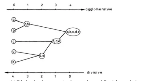
Figure 14 Distinction between Agglomerative and Decisive techniques ... 43

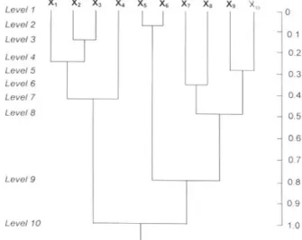
Figure 15 A simple dendrogram for hierarchical clustering... 44

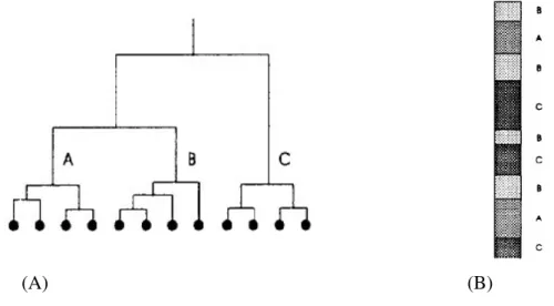
Figure 16 Showing of four hierarchical algorithms methods ... 47

Figure 17 Dendrogram showing clustering scheme resulting in four class. ... 49

Figure 18 Stages of Cluster analysis of log data: (a) dendrogram of zones according to hierarchical clustering of zones based on their similarities; (b) classification of zones ... 50

(9)

9 Figure 20 The dendograms of well A1,B2, and C3. ... 53

Figure 21 Box plots showing distributions of the gamma ray values within four electrofacies classes determined by clustering on log data... 56

Figure 22 Well log data with depth intervals for two selected wells. a) Well T20, b) Well U21 62

Figure 23 Profile of four electrofacies at Well T20 ... 62

(10)

10

LIST OF TABLES

Table 1 In-place reserve for Canada’s bitumen deposits (Alberta Energy and Utilities Board, 2006) ... 30

Table 2 Stratigraphic Nomenclature and Characteristics of Different Units in Athabasca

Wabiskaw-McMurray Succession, Northeastern Alberta... 55

Table 3 This shows the statistical values of the computed box plots indicating the values of the lower end of the whisker, the first quartile (25th percentile), second quartile (median=50th percentile), third quartile (75th percentile), and the upper end of the whisker... 57

(11)

11

1. INTRODUCTION

The geophysical wireline log measurement acquired from the drilling of densely distributed

wellbore in the Athabasca Oil Sands of Alberta, Canada requires expert geological knowledge

for its interpretation. It requires manual analysis which is time consuming especially when the

wellbores are numerous thereby making an automatic analysis more important in Oil and Gas

exploration. Pattern recognition methods are used to identify the patterns of the wireline log

reading from wellbore. This thesis explores the opportunity of automating the interpretation and

analysis of well log data of gamma ray logs using a statistical pattern recognition approach.

1.1. Problem Statement and Motivation

A crucial problem in oil and gas exploration industry is the interpretation of the measurement of

the physical properties of particular underground rocks such as density, electrical resistivity,

sound transmission, radioactivity etc. These measurements are called logs and are characteristic

of the various rocks penetrated by the drill. However, wellbore analyses from the massive

volume of data as a result of different types of surveys and continuous well logging are

constantly practices in the oil and gas exploration industry. The idea of efficient techniques to

process such large volume of data have brought about the concept of an automated technique to

refine the data (trace editing and filtering), select the desired event types (first-break picking) or

automated interpretation (horizon tracking) for effective geological data interpretation. These

have been proven to be particularly interesting to apply in stratigraphic interpretation as well as

correlation. Nikravesh and Aminzadeh (2003) explain how the mining and fusion of reservoir

data are utilized in the soft computing techniques for intelligent reservoir characterization. Most

existing computerized well-log interpretation systems deal with maintenance of a well-log

database and evaluation of formation fluid, but rarely with a stratigraphic interpretation (Wu and

Nyland 1987). Over the past two decades, geosciences have experienced developments and

application of numerous quantitative approaches ranging from spectral to cluster analysis.

Agterberg and Bonhan-Carter, (1990) and Agterberg and Griffiths, (1991) describes how these

approaches have found wide application throughout geosciences and have been used for process

simulation, modeling, mapping, stratigraphic analysis and correlation, classification and

(12)

12 The expert geological knowledge in the analysis and interpretation of the oil sand well logs are

of paramount importance. However, the manual analysis can be time consuming especially when

the well log data are obtained in a large number of densely distributed wellbores. Therefore, the

possibilities of automating the interpretation and correlation of these well-log datasets to build a

subsurface model are very helpful in Oil and Gas exploration. It is also possible that

computer-assisted correlations may suggest zonal matches of interest and originality that might not have

been considered during the manual analysis. Different approaches have been explained by

several authors ranging from statistical methods to Pattern recognition and Artificial Intelligence,

all leading towards an automated extraction of information from signals. The term ‘signal’ is

broadly interpreted to include well log data, waveforms, images and other survey data. This work

will utilize the approaches of pattern recognition and artificial intelligence in an attempt to

automatically interpret and correlate well-log datasets from Athabasca Oil Sands of Alberta,

Canada. This area has about 250,000 wellbores and obviously is a real challenge in performing

manual analysis.

Sequel to the above, the sample well data set of Exeler,(2009) work and the general geological

knowledge of Athabasca Oil Sands were utilized for the prototypical implementation of an

automated stratigraphic interpretation using well log data set within this Master thesis.

1.2. Oil Sand in Athabasca

The term Oil Sand can be defined as crude deposits which are substantially heavier (more

viscous) than other crude oils consisting of sand, bitumen, mineral rich clays and water.

Bitumen is a product of the oil sands that requires upgrading to synthetic crude oil or dilution

with lighter hydrocarbons to make it transportable by pipelines and usable by refineries. Hence,

the crude bitumen together with the reservoir rocks where it is found is known as Oil Sands

(C&C Reservior 2007).

The base of the Canadian Oil Sand Reservoir is located in the north-east Alberta which

comprises three major deposits, illustrated in (Figure 1): the Peace River Oil Sands, the

Athabasca Oil Sands and the Cold Lake Oil Sands. According to the Alberta Department of

Energy (ADE, 2006) the Oil Sands deposits were evaluated to contain approximately 1.7 trillion

(13)

13 recovered using current technology. The proven oil reserve in Alberta accounting up to 15% of

the world reserve is second after Saudi Arabia (ADE, 2006).

HILLS, (1974) explain that the Oil Sand formations of Northern Alberta represent a vast source

of fossil fuel whose exploitation is of major economic importance compared to the conventional

crude oils.

Figure 1. The major deposit: the Peace River Oil Sands, the Athabasca Oil Sands and the Cold Lake Oil Sands Adapted from (C&C Reservior 2007)

In Athabasca, the area of interest for development contains thick bitumen-saturated sands which

generally have good lateral continuity and excellent permeability. The geological formation that

contains this bitumen is explained in section 3.2. Recovery of these bitumen (reservoir sands)

(14)

warm-14 flotation (in areas where overburden thickness is less than 75 meters) and by in situ thermal

techniques like the steam-assisted gravity-drainage (SAGD) process especially in areas where

the Oil Sands are deep suited.

Generally the recovery factor for surface mining and in situ thermal techniques are estimated to

be between 80% and 60% respectively (C&C Reservior 2007). It is essential to note that around

250,000 wells have been drilled in this area since 1945 which have been cored and measured

with petrophysical wireline logging.

1.3. Objectives

The general objective of this thesis aims at recognizing the patterns of the available well log

dataset (Gamma ray data) to describe and interpret the stratigraphy by automating the

classification and possible correlation process. This is done by considering the coherent grid of

well logs from 21 wellbores made available for the study area. This spatial data may allow in

deriving a model of the subsurface by integrating the geological knowledge of the area. The

analysis will focus on determination of the electrofacies of the individual wells and delineating

the sandbodies which serve as the reservoir rock for the bitumen. In the first step, the

geophysical log data of each individual well will be examined, analyzed and partitioned, here

gamma ray logs, using the developed clustering algorithm. The clustering aims to classify the

data and subsequently depict different rock types. The difference of each gamma ray data will be

re-computed and clustered for each well in order to recognize all the hidden patterns of the log

data, which the original log data and the first clustering fails to recognized. In the second step,

the gamma ray log data limit of each clustered well will be computed. This will be based on the

similarity matrix index of each well. The optimal number obtained which is explained in section

5.2 will be utilized in determining the electrofacies of each individual wells and subsequently

construct the lithology of each well. The whole process will be automated so that all the

wellbores are clustered automatically and the electrofacies of each well will be generated. In the

third step, a set of decision rules will be generated based on the mean gamma ray and the

maximum value of gamma ray in each cluster. The idea is to automatically assign lithology

facies in each electrofacies classification. The electrofacies and the lithology will identify the

sand, shale and intermediate sediment. The spatial relations between the individual wells will be

(15)

15

1.4. Scope of the Research

The thesis investigates a pattern recognition approach utilizing clustering algorithms for the

interpretation of geological well log datasets. This approach tries to classify different rock types

in the subsurface leading to the determination of a refined geological stratigraphy that will

identify shale, sand and intermediate sediments from the well log dataset automatically. The

implementation focuses on the depositional environment of the study area and this can be applied

to different depositional environments in the future. It can be argued that the result of an

automatic subsurface model from well log cannot replace human expertise due to the complexity

of geological processes, but will definitely speed up the analysis process especially in large data

sets from numerous wellbore.

1.5. Research Hypothesis and Question

1.5.1. Hypothesis

The hypothesis of this study is stated as: Pattern recognition approaches based on utilizing

clustering algorithm can be used in classifying and interpreting stratigraphic column

geologically, which promotes synergy for well correlations.

1.5.2. Research Questions

In order to meet the hypothesis and objectives of this study, the following research questions

were set.

• _{Are the patterns from the well log data of the study area to recognizable?}

• _{How can these patterns be recognized and automatically be utilized in the subsurface}

stratigraphic interpretation?

• _{Does this form the basis for correlation?}

1.6. Thesis Structure

In this thesis the problem of pattern recognition of well log data utilizing clustering algorithm for

the identification, classification and interpretation are considered. The reminder of the thesis is

structured as follows:

The second section will provide an overview of related work in the field of well log cluster

analysis, interpretation and correlation. It will also discuss the techniques and methodology of

pattern recognition. In section three, the study area and general geological background will be

(16)

16 system and stratigraphy. Section four will explore the dataset provided for this thesis, it will

describe the well location and spatial distribution of the wells, considering the dimension and

resolution of the wells. In section five the methodological framework of the stratigraphic

interpretation of oil well log data will be described. It will elaborate on the steps of clustering

analysis and the computation processes. Section six will illustrate the prototypical

implementation of the described methods with the statistical programming language R. The

results will also be evaluated in this section. Lastly, the discussion and conclusion will be

(17)

17

2. RELATED WORKS

The recognition of signal patterns generated during wellbore measurements is paramount in

exploring for economically viable accumulations of hydrocarbon. Stratigraphic signals require

analysis of its large volume of data. This enables the development of an extensive knowledge of

its interpretation within reservoir distributions. Several techniques have been proposed and

developed to interpret these signals (well logs) computationally, as the basis for reservoir model

constructions from well log data. It comprises classification of logs, determination of

electrofacies and inter-well correlation of the identified facies.

2.1. Well Log Cluster Analysis

A well log can be described as a record of the characteristics of rock formation against depth (see

section 4.3 for further details). Cluster analysis starts with the partitioning of data into

meaningful subgroups, when the number of subgroups and other information about their

composition may be unknown. The methods range from those that are largely heuristics to more

formal procedure based on statistical model (Fraley and Raftery, 1998).

Euzen, et al.,(2010) utilizes a method in seeking high density areas (clusters) in the multivariate

space log data, in order to define classes of similar log responses thereby determining and

classifying electrofacies. This was applied to develop unconventional gas prospect in the Upper

Mannville incised valley fills of the Western Canadian Sedimentary Basin. Performing an

electrofacies zonation based on attempt to identify clusters of log values coming from similarity

level with the same characteristics has been carried out in the works of Wolff and

Pelissier-Combescure, (1982); Delfiner, et al., (1987); Lim, et al., (1997); Lee, et al., (2002) and Lim,

(2003). They attempt to utilize all available wireline log data set, which was against the

conventional norms of using only one log, often resistivity log or gamma ray log. These logs data

sets are corrected and are selectively reduced via a procedure known as principal component

analysis. The first principal component computed which is a dimensionless log containing the

largest common part of variances of the input logs was clustered. The clustering attempts to

reduce the input log to a set of clusters which are meaningful and each cluster can be related to a

specific geological facies.

Gill, et al., (1993) Partitioned a suite of well logs into geologically meaningful zones by a

proposed numerical multivariate clustering. Zones and logfacies were discriminated by

(18)

18 minimal. Lee, et al., (2002) proposed a hierarchical agglomerative clustering technique known as

Model-based clustering to classify log data. The author noted a better performance than

single-link (nearest neighbor) and k-mean clustering which often fail to identify groups that are either

overlapping or of varying sizes and shapes

An automated pattern classification of well log data through different neural and non-neural

techniques such as self-organize vector quantization to categorize lithological profile and

determine electrofacies have been proposed by (Hassibi, et al., 2003). Vector quantization is an

unsupervised clustering technique based on distance functions within Euclidean space.

2.2. Well log Correlation

After the clustering and electrofacies determination or zonation of well logs, logs can be

correlated to build a geological model. These correlations are generally done manually (Schaefer,

2005). However, different methodologies have been proposed to automate this process

(Gradstein et al., 1985; Tipper, 1988; Olea, 1994; Hassibi et al., 2003).

Conventional method that utilizes mathematical correlation in the space and frequency domains

is reviewed in (Hoyle, 1986). Olea (1994) developed a rule based Expert Systems for automated

correlation. The same approach was proposed by Lim et al., (1999) in their rule-based inference

program in correlating zones between wells. Wu and Nyland (1987) applied dynamic sequence

matching by coding sequence into lithofacies.

Exeler, (2009) Proposed a topological approach for the interpretation of geological well log data

by integrating geological knowledge and well topology into an automatic classification and

correlation process. Hassibi et al., (2003) performed similarity characterization of reservoir via

pattern recognition approach which delineates dominant reservoir compartmentalization. Lateral

continuity correlation of logs was performed by an Expert System.

2.3. The Theory of Pattern Recognition

Pavlidis, (1977) defines pattern recognition as involving the identification of particular structures

which a given object is composed of. These objects are inspected for “recognition” process

which turns into classification (Friedman and Kandel, 1999). Pattern class reflects a set of

patterns that have in common some similar characteristics. To recognize a pattern, one can use a

model such as self-organizing networks (Kohonen, 1997) or fuzzy c-means techniques (Bezdek,

(19)

19 to recognize the topology, patterns, or seismic objects and their distribution in a specific set of

information.

The science of pattern recognition is concerned with three major issues (Pao, 1989).

• _{The appropriate description of objects, physical or conceptual, in terms of representation}

space;

• _{The specification of an interpretation space; and}

• _{The mapping from representation space into interpretation space}

Furthermore, pattern recognition sciences can be exemplified as follows:

a. Classification: This tries to assign input values to one of a given set of classes. It

implements a procedure that learns to classify new instances based on learning from a

training dataset of instances with correct classes. Commonly known as supervised

classification. The corresponding unsupervised procedure is known as Clustering which

involves grouping of data into classes or finite set of categories according to their

similarity relations.

b. Regression: This assigns a real-valued output to each input

c. Sequence labeling: This assigns a class to each member of a sequence of values (for

example, part of speech tagging which assigns a part of speech to each word in an input

sentence); and

d. Parsing: This assigns an input sentence a parse tree describing the syntactic structure of

the sentence.

From a broad perspective, pattern recognition techniques can be classified into two major

categories—the conventional approach and the artificial intelligence (AI) based approach.

Conventional techniques are based upon two major methodologies known as statistical and

structural pattern recognition (Nandhakumar, and Aggarwal, 1985).

2.3.1. Statistical Pattern Recognition

A statistical Pattern Recognition scheme provides for the classification of the signal into one of a

finite number of classes for each of which a multivariate probability distribution function is

assumed to exist, especially when the various distribution functions of the classes are known.

The method tries, in most cases, to model the class distributions and also to find a discriminant

function that minimizes the classification error. Modeling class distribution is based by two

(20)

20 i. Supposing that the class distribution comes from a known family of distributions

ii. Letting the data from the class distributions.

These approaches are categorized under parametric and non parametric method as explained in

(Duda and Hart, 1996).

It is essential to note that a statistical classifier must be able to evaluate risk associated with

every classification which measures the probability of misclassification.

The Bayes classifier based on Bayes formula from probability theory minimizes the total

expected risk (Friedman and Kandel, 1999). The distribution function may be known a priori or

it may be estimated from a training datasets. A classifier uses the feature values evaluated for a

particular signal to assign the signal to a class. Typically, the classifier is designed with the

criterion of minimizing the Bayesian error probability, or a cost measure based upon it. There are

some exceptions to this which is termed template matching. Nandhakumar and Aggarwal, (1985)

explain how the data being examined and the template that is being used are considered to be

vectors, which utilizes a metric (e.g. the Euclidean norm) in measuring the similarity, or

distance, between the two vectors. Statistical Pattern Recognition techniques are domain

independent in that the algorithms can easily be transported to different domains provided that

some encoded heuristics are followed.

Wu and Nyland (1987) explain that stratigraphic interpretation begins with zonations and zone

correlation in which the statistical algorithms are utilized and the major interpretation is based

upon maximum cross-correlation of zones in two wells. This supports the explanations of Huang

and Williamson (1994) which affirm that the quantitative approaches applied in geosciences in

analyzing log datasets are statistical in nature. Its application has permitted systematic, rapid and

objective analysis and processing of dataset.

2.3.2. Structural Pattern Recognition

Structural Pattern Recognition schemes are based on defining primitives (substructure

relationships) and identifying allowable structures. It represents an attitude rather than a specific

set of procedures which involves the following processes (Nandhakumar and Aggarwal, 1985):

• _{identifying and extracting morphs}1_{(segmentation, symbol designation);}

1

(21)

21

• _{identifying relationships between morphs in allowable structures (defining the}

syntax/semantics);

• _{designing an algorithm for recognizing the occurrence of a structure of morphs in terms}

of the derived relationships (designing a parsing strategy)

It is essential to note that a signal may be considered to be made up of an arrangement of morphs

(-segements of specific shapes like parabolas, straight lines etc) and the final goal of a structural

pattern recognition is the detection of structures.

2.3.3. Artificial Intelligence

Artificial Intelligence (AI) is seen as a collection of advanced computing techniques developed

to solve problems that humans can easily solve but are very difficult for conventional computing

techniques (Baker, 1989) and also the development of computational models of intelligent

behavior, including both its cognitive and perceptual aspect (Duda and Shortliffe 1983). It

involves the description of abstract concepts (represented by several/ hierarchical levels of

abstraction) and the recognition of instances of the signals (Nandhakumar and Aggarwal, 1985).

Researchers from different disciplines have been attracted to this study. They have considered

the fascinating power of the brain formed by very simple cells called neurons in controlling body

action, processing signals, making decision, and information storage. A neuron can therefore be said to be a specialized cell capable of processing the incoming information and conducting itto the next neuron. Kandel, et al.,(1991) and Nicholls, et al., (1992) explained in details the processing phase. The idea of copying the brain and neuron forms the basis of AI and is pioneered by the works of McCulloch and Pitts, (1943); Pitts and McCulloh, (1947), Rosenblatt, (1958) and Hebb, (1949).

It is essential to note that Artificial-intelligence researchers have tried also to cast the visual

perception problems in the domains of symbolic representation, symbolic structures, and

symbolic processes to facilitate the symbolic representation of arbitrary objects and the

relationships among them. This has resulted to the broad division of Artificial Intelligence into

two basic categories:

a. Rule-based (expert) systems

(22)

22

2.3.3.1. Rule-based (expert) systems

This is commonly known as knowledge-based, which involves reasoning. Reasoning, however,

involves drawing inferences from information, provided that data are in an appropriate

representation scheme. The reasoning procedures work as programs manipulating data

syntactically to deduce new programs following pre-specified rules of inferences. Hence, the

computer programs formulated this way exhibit what is generally considered as intelligent

behavior. This type of computer software system is called a rule-based system (Startzman, et al.,

1987). This author also noted its successful application in many areas, including computer

configuration, diagnosis of infectious diseases, mineral deposits prospecting, log interpretation,

and drilling-mud consultation.

2.3.3.2. Adaptive (neural) system

Artificial neural systems, or neural networks, are physical cellular systems that can acquire,

store, and use experiential knowledge. The knowledge is in the form of stable states or mapping,

embedded in networks that can be recalled in response to the presentation of cues. Hence, unlike

a digital, sequential computer with a central processor that can address an array of memory

locations, neural networks store knowledge in the overall state of the network after it has reached

some equilibrium condition (stable state), thereby storing not in a particular location

(Mohaghegh, et al., 1996). Neural networks have pattern recognition and adaptability as its

proven strong points. The essence of pattern recognition is the concurrent processing of a body

of information, all of which are available at the same time (Mohaghegh, S., et al 1996)

The geological application of Artificial Intelligence introduced in the work of (Simann and

Aminzadeh, 1989) have recorded success to the numerous challenges posed in the quantitative

analysis and interpretation of geological data and had since been further developed.

Wu and Nyland (1987) state that a computerized well-log stratigraphic interpretation system

based on artificial intelligence can be seen as two steps, contact recognition and interval

identification which considers geologic environment for effective interpretation. The system

(well-log interpretation using artificial intelligence techniques) developed by Wu and Nyland is

(23)

23

Figure 2 A schematic of the design of Artificial Intelligence in well-log interpretation Adapted from (Wu and Nyland 1987)

In this study, Statistical Pattern recognition and Rule-based system (Artificial Intelligence)

methods will be used. This is because of the nature of the sample data.

Secondly, statistical pattern recognition allows a priori geologic knowledge to be inserted into

(24)

24

3. THE STUDY AREA

This section describes the sedimentary environment of deposition, the general geological setting,

and the sequence stratigraphic framework of Athabasca Oil Sand where the exploration is done

through drilling sizeable quantities of densely distributed wellbores. The output of the drilling

amounts to large datasets that requires quantitative analysis.

Sequel to the objective set for this thesis which explores the concepts of an automated

interpretation of well log data from Athabasca Oil Sand through pattern recognition, the detailed

knowledge of the geology is significant for the interpretation approach described in section 5.

3.1. The Sedimentary Environment and General Geological Setting

A sedimentary Environment describes the combination of physical, chemical and biological

processes associated with the deposition of a particular type of sediment. It also describes the

rock type formation after lithification if the sediment is preserved in the rock record.

The Sedimentary environment can be divided into various classes which includes alluvial fans,

rivers and flood plains, marginal-marine (deltas, alongshore sand bodies), and marine (shelf,

submarine fans, turbidite sequences) (see figure 10). According to Hassibi et al., (2003) deep

marine environments are mostly formed by turbidity flows and its facies especially those

comprising fan channels and lobes, constitute some important hydrocarbon reservoirs worldwide.

It is important to note that heterogeneities are bound to occur in turbidite reservoirs which can be

as a result of the lobes to the source material. The nature of sand lobes determines the vertical

and horizontal variations in the sequence thereby making sand continuity and lateral correlation

an important issue.

The Athabasca Oil Sands Area is located in the Western Canada Sedimentary Basin, north-east

Alberta Canada (Figure 1, Section 1.2). The area is one of the several bitumen-producing areas

that occur along the eastern margin of the western Canada Sedimentary basin (C&C Reservoir,

2007). The Western Canada Sedimentary Basin (WCSB) covers an area of 1, 400,000 Km2 and

stretches from the Proterozoic crystalline basement of the Canadian Shield in the north-east to

the Cordilleran fold-thrust belt in the south-west. According to Alberta Geological Survey,

WCSB can be divided into two distinct parts, reflecting sedimentation in two profoundly

different tectonic settings.

(25)

25 ii) The clastic rocks dominated overlying mid-Jurassic to Paleocene foreland basin

succession

The former was deposited on the stable craton adjacent to the ancient (dominantly passive)

margin of North America while the later was formed during active margin orogenic evolution of

the Canadian Cordillera. This explains the three phases of the geological history of the Western

Canada Sedimentary Basin (WCSB) according to (C&C Reservoirs, 2007) which includes the

following: :

1. Cratonic platform (Precambrian-Middle Jurassic)

2. Retro-arc foreland basin (Middle Jurassic-Eocene)

3. Intracratonic basin (Eocene-present).

During the Precambrian to Middle Jurassic, the WCSB lay on the western flank of the North

American continent as part of the cratonic platform. Price (1994) stated that the WCSB was

affected by block faulting and volcanism associated with subduction beneath an oceanic volcanic

arc lying outboard of the continental margin during the Lower Paleozoic period and in this phase

clastic detritus came mainly from the east. The Antler Orogeny in the USA was linked to the

basin’s extension and rapid subsidence in the late Devonian-Early Mississippian. In the middle

Jurassic, Columbian Orogeny occurred as a result of eastward subduction resulting in regional

angular unconformity. It is essential to note that the locus of maximum subsidence migrated

north-east as the accretionary prism prograded eastward onto the flank of the continental craton.

An episode of crustal extension in the Eocene in the Cordillera marked the transition to the

present-day intracratonic tectonic regime. From the Eocene onward, the WCSB was

progressively uplifted, with as much as 1 km of uplift occurring by the Quaternary (C&C

Resevior, 2007). The basin contains a wedge of Middle Proterozoic to Eocene sediments that

pinches out into the Canadian Shield and thickens to >6 km adjacent to the thrust front in SW

Alberta (Wright et al., 1994).

3.2. Petroleum System and Stratigraphy

The Pre-Cretaceous regional angular unconformity of Athabasca lies below the Lower

Cretaceous (Aptian-Albian) Mannville Group deposit (Fig. 3A). The north-northwest trending

regional valley was created as a result of the dissolution of salt in the Elk Point Group and

collapse of carbonates in the overlying Beaverhill Lake Group within the subcropping Middle

(26)

26 (Figures 3 and 4). This valley is commonly called the Main Valley which bordered to the west by

a carbonate-cored anticline, known as the Athabasca Anticline and served as a major feature in

the Athabasca area in the Early Cretaceous (figure 5). During a marine transgression in which the

Boreal Sea invaded the Alberta Basin from the north-west, sediments of the Lower Mannville

Group (Aptian McMurray Formation) were deposited in the erosional valley. At this moment,

the Alberta Basin was bounded on the west by the rising Cordillera and continental sediments

eroded from this mountain chain entered the Main Valley from the south, beyond the southern

terminus of the Athabasca Anticline (figure 5). Above the unconformity surface, fluvial

channel-fill sandstones of the lower McMurray Formation were directly deposited by the river flowing

northward along the valley axis.

As the sea level rises, the Upper Mannville Group (Wabiskaw Member of the Clearwater

Formation) was deposited above the McMurray Formation which was covered by upper

Clearwater marine shales. The great majority of bitumen in the Athabasca area is entrapped in

the McMurray/ Wabiskaw interval. The Clearwater shales are overlain by marine

shelf/shoreface, delta-front and delta-plain deposits of the Grand Rapids Formation, which

comprises the upper portion of the Mannville Group and consists of multiple prograding deltaic

cycles topped by marine flooding surfaces. (C&C Reservoir, 2007).

Figure 3A depicts the bitumen generation of Athabasca from the Devonian-Mississippian

Exshaw Shale, which occurs beneath the regional angular unconformity that underlies the

Mannville section. The Exshaw was deposited on an anoxic marine shelf containing Type II

kerogen with TOC values of 10-20% and hydrocarbon indices of 400-600. During the uplift and

uncapped episode in the mid-Tertiary, hydrocarbon expulsion ceased. However, most bitumen

trapped in the Athabasca migrated out of basin as oil and entered shallow stratigraphic and

structural traps in the Late Cretaceous-Paleocene Laramide deformation. The oil was

subsequently water-washed and biodegraded to form bitumen.

The occurrences of bitumen in three reservoir rocks of Athabasca have been identified in the

Lower Cretaceous McMurray, Wabiskaw Grand Rapids deposits and the Devonian

Grosmont/Nisku deposit. The heavy viscous oil is contained in a shallow stratigraphic-type trap

formed by the McMurray Formation and the overlying Wabiskaw Member of the Clearwater

(27)

27 The Lower McMurray fluvial succession is preserved mostly parallel with lows on the

sub-Cretaceous unconformity, and contains mainly bottom water. Figure 3 shows the development

such as the in-situ projects going on in these areas. Flach and Hein, (2001) described the Joslyn

Creek in-situ project which target bitumen in Lower McMurray braided river-sand reservoirs

where the reservoir comprise sand-dominated, channeland- bar complexes, having high

porosities and permeability, high interconnectivity and lacking internal barriers or baffles

The overlying Upper McMurray succession is a transgressive systems tract that contains some

of the richest bitumen reservoirs within the Athabasca deposit, hosted mainly within

amalgamated or stacked estuarine channel-and-point bar complexes. These reservoirs include

thick (up to 58-m) estuarine channel sands with no laterally extensive shale breaks.

In summary, the Cretaceous McMurray Formation of the Athabasca Oil Sands was deposited on

the eastern, low-accommodation side of the foreland-basin. Reservoirs, 10–90 m thick, occur in

tidally influenced meandering point-bar and tidal-bar deposits. The reservoir occurs at depths of

0 to 400 m a combination of structural-stratigraphic trap by viscous immobility, depositional

pinchout, and subtle anticlinal closure (C&C Resevior, 2007).

The sediments were mainly derived from exposed craton to the east and northeast with the

minimum sediment burial and early oil migration resulting in 30–35% porosity and multi-Darcy

permeability. The variation of the reservoir and the bitumen parameters are identical.

According to Norsk Geologisk Forening, microbial biodegraded bitumen of Athabasca varies

from 6–8º API gravity with greater than 1,000,000 cP viscosity, which can also vary by an order

of magnitude over 50 m vertical and 1 km laterally. However, the shale layers (mud plugs),

extensive tidal flat or muds on laterally accreting point bars posses a manageable challenge to

bitumen development. The oil source is likely Mississippian shale of the Exshaw Formation (see

Fig. 4) from the underlying passive margin succession, which reached maturity during foreland

basin compression. Work by others suggests that the Exshaw oil may have been generated and

(28)

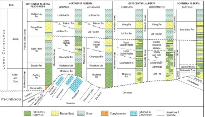
28 Figure 3 – (A) SW-NE schematic structural cross section showing distribution of Athabasca, Wabasca and Peace River oil sand in the Lower Cretaceous Mannville Group and their

(29)

29 Figure 4 Lower Cretaceous stratigraphy of Alberta, showing unconformable relationship of the Cretaceous section to the underlying Paleozoic section. Adapted from (Keith et al., 1988)

(30)

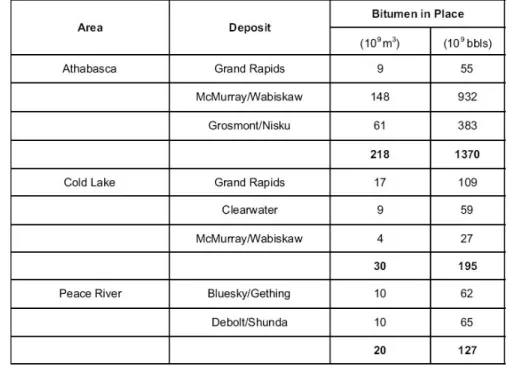
30 Table 1 shows the percentages of bitumen reserve represented as 68% and 32% respectively,

contained in the Lower Cretaceous sandstone of the Mannville Group and the underlying

Devonian carbonate of the Grosmont and Nisku formation. The Mannville Group of Athabasca

oil Area comprises, in ascending order, the Aptian McMurray Formation, the Albian Clearwater

Formation and the Albian Grand Rapids Formation. The McMurray is dominated by

fluvial/coastal-plain sandstones and the Clearwater by marine-shelf shales and was deposited

directly upon a Cretaceous angular unconformity underlain by Paleozoic carbonate rock (Figure

3) (C&C Resevior, 2007). Wabiskaw Member directly overlies the McMurray Formation which

comprises a thin interval of marginal-marine glauconitic sandstones and shales. Hence, in the oil

sand of the Lower Cretaceous Manville Group, 94% of the bitumen reserves occurred in the

McMurray/Wabiskaw deposit while the remaining 6% are found in the Grand Rapid reservoir.

Table 1 In-place reserve for Canada’s bitumen deposits (Alberta Energy and Utilities Board, 2006)

(31)

31 Figure 6 Response of gamma ray to different depositional environment (Modified from Tsai-Bao Kuo. 1986).

Athabasca deposit is hosted within fluvial, estuarine, and marginal marine deposits of the Lower

Cretaceous Wabiskaw-McMurray succession (Hein and Cotterill, 2006). Figure 6 shows

different response of gamma ray to different depositional environment. It essential to note that

different depositional environment have different characteristic log response and the higher the

gamma ray units the sandy the signature.

Flach and Mossop (1985) describe the stratigraphic pattern of the northern portion of the

Athabasca Oil Sand Area has the McMurray Formation divided into lower, middle and upper

members. The thickness of the lower member is between 0-60m with an overall fining-upward

profile and consists of medium- to coarse-grained sands, arranged in 5-10 m thick, fining-upward

packages, interbedded with carbonaceous mudstones and thin coals that are common near the top

(Figure 7). The middle members is approximately 40m thick and consist of channel facies and

(32)

32 argillaceous sand and shales that are local truncated by channel-fills. Some sand intervals near

the top of the upper member were interpreted as marine offshore bars (Figure 7B)

Figure 8 describes the detailed interpretation of a gamma log. Thus, this thesis will explore the

possibilities of recognizing the signature of the sand bodies (sand intervals) with different grain

size and also shale intervals (which are more laterally extensive) from the given gamma ray

datasets in order to investigate the connections. This will enable the complete stratigraphic

interpretation and correlation.

(33)

33 Figure 7 – N-S (A) and W-E (B) stratigraphic cross-sections of the McMurray

(34)

34 Figure 8 An automated interpretation of gamma log. Adapted from (Wu and Nyland 1987)

(35)

35

4. STUDY DATA

This section provides a brief description of the sample data available from the study area. These

sample dataset were used to test the electrofacies determination/ interpretation approach of this

thesis. The well logging techniques utilized in the wells of the study area are also described in

this section.

4.1. The Sample Data Set

The sample dataset available for this study are the well logs of Gamma ray, Dipmeter and

Azimuth. It is provided from 21 wellbores from the study area, with the down-hole penetration

(depth) varying between 75 and 101 meters. The depth values were adjusted to a common

reference level and hence remain a relative depth representation. The log of each wells are read

approximately at every 10cm down-hole in which the readings of gamma radiation, the azimuth

and the dip are recorded. However, for the purpose of this study, only the dataset of gamma ray

were utilized after an extensive discussion with an expert geologist from Shell International

Exploration and Production, The Netherlands.

4.2. Well Distribution

The sample data is unevenly distributed of the sample dataset in an area of about 15Km2(Figure

9). The distance between two adjacent wells varies to a large extent between 300 and 2000

meters. The sample dataset were georeferenced in a UTM projection based on WGS84, given the

well location in a metric Cartesian coordinate system (Exeler, 2009). It is essential to note that

the coordinates represented in this thesis are not original absolute coordinates, instead it shows

relative positions and the original coordinates were changed for anonymity reasons.

4.3. Well logging

A well log is simply described as a recording of characteristics of rock formation against depth.

It is carried out for reservoir characterizations where measurements of the physical properties of

surrounding rocks are with a sensor located in a borehole are recorded (Telford et al., 1990). The

principal aims of these tasks include the following

a. Identification of geological formations

b. Identification of fluid formation in the pores

(36)

36 Figure 9 Relative well locations of the sample data. Adapted from Exeler, (2009)

The geological investigation of formation thickness (Lithology), porosity, permeability,

saturation water and hydrocarbon usually combines about five well logging such as Electrical

resisitivity logging, Radioactive logging (Gamma ray and density logging), Auxiliary logging

(Includes sonic logging), Dipmater logging, Azimuth logging etc. (Telford et al., 1990). The

changes which are projected on a well log imply that well log signals are function of sedimentary

patterns. Figure 10 depicts a sedimentary pattern. It shows a 3D model that indicates the

development of a submarine fan and the variation of sedimentation in different location. For the

(37)

37 Figure 10 3D model of a sub marine fan. (Adapted from Shanmugam et al., 1988)

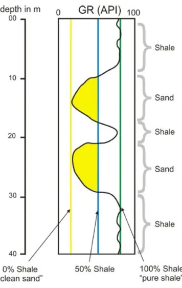
4.3.1. Gamma ray logging

Gamma radiation is used for qualitative evaluation of shaliness or clay content of a formation by

measuring the natural radioactivity of the formation adjacent to the wellbore. Shale emits more

gamma radiation than non shale sediments such as shale free- sandstones and carbonates because

its gamma ray reading is high, since the concentration of radioactive material is high. Gamma

ray logs are used in identifying lithologies, correlating formations and calculating volumes of

shale. It is recorded in a relative scale using American Petroleum Institute (API) units. Figure 8

(38)

38 Figure 11 Interpretation of a gamma ray log. Adapted from Exeler, (2009)

(39)

39

4.3.2. Dip and Azimuth

Dipmeter logging tools records high-resolution conductivity curves from multiple pads pressing

against the borehole wall (Baker, 1989). Dipmeter tools determine the structural dip and azimuth

in wells with an accuracy of plus or minus two. Dipmeter logs have a high vertical resolution of

3 to 5 cm with the depth of investigation is approximately 1 cm. Figure 12 describes the azimuth

(40)

40

5. METHODOLOGICAL FRAMEWORK FOR THE STRATIGRAPHIC

INTERPRETATION OF WELL LOG DATA

The stratigraphic interpretation procedures of the well log data applied to this thesis is described

in the flow chart of figure 13. The first two steps examine the individual wellbore. The

explanation of the processes and the logic behind applications is explained below.

5.1. Recognition of Lithofacies and Electrofacies

Recognition of lithofacies is a common practice in drilled wells where suitable well logs and

core samples are available. Pattern recognition techniques such as hierarchical and k-means

cluster analysis can be used for classifying well log data into discrete classes. The automation of

well log correlation using both multivariate statistical techniques including principal component

analysis (PCA) and rule based system for efficient and reliable pattern recognition for

well-to-well correlation can be established. Lim, (2003) used the first principal component log, since it

has the largest common part of variance of all available well log data.

The key to an automated interpretation of pattern is to explore the logic of human interpreters

and follow this logic in designing the computer software. Correlation (of wireline logging data)

is also based on the large set of subjective rules for pattern recognition that aims to represent

human logical processes. Following the foregoing, statistical pattern recognition methods was

utilized in this work. This is based on numerical computation procedures (mathematical

calculation) in identification of patterns.

The advantages of this approach are that (Nikravesh, et al., 2003; Lim, 2003).

• _{It can be applied in all depositional environments,}

• _{It can be more helpful for obtaining more reliable correlation results for complex}

geologic formation

• _{It has the capability of dealing with probability and uncertainty of data due to fuzziness}

The geological information that is meaningful can be derived by selecting, weighting and

combining a set of logs which give rise to a set electrofacies that can be correlated with

(41)

41 An electrofacies is defined as the set of log responses which characterizes a bed and permits it to

be distinguished from others (Serra and Abbott, 1982). In log-analysis applications, an

electrofacies is used typically as an indicator of lithology and depositional environment (Wolff

and Pelissier-Combescure, 1982; Anxionnaz, Delfiner, and Delhomme, 1990). Electrofacies

zonation is based on the attempt to identify clusters of log values coming from levels with

similar characteristics. The importance of electrofacies characterization in reservoir description

and management has been widely recognized as this kind of data partitioning is to simplify a

complex data set into some homogeneous and simple subgroups and to produce a better

correlation between dependents and independents within distinct subgroups for further

petrophysical properties regression (Lee and Datta-Gupta, 1999). The electrofacies

determination procedure which is based on cluster analysis of well logs used in this study is

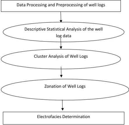
summarized by the flow chart in figure 13.

Figure 13. Flow Chart of electrofacies determination Data Processing and Preprocessing of well logs

Cluster Analysis of Well Logs

Zonation of Well Logs

Descriptive Statistical Analysis of the well log data

(42)

42

5.2. Cluster Analysis of well logs

The provided well data comprise the readings of gamma radiation, azimuth and dip taken at

about every 10cm of the total well depth. This makes the reading too detailed that sediment

classification has the tendencies of overlapping. However, samples with similar logs responses

need to be identified. This identification is done using a clustering algorithm that can operate on

log traces.

Cluster Analysis, also called data segmentation, relates to grouping or segmenting a collection

of objects (observations, individuals, cases, or data rows) into subsets or "clusters", such that

those within each cluster are more closely related to one another than objects assigned to

different clusters. The purpose of cluster analysis is to look for similarities/dissimilarities

between data points in order to group them into classes. In multi-dimensional space logs, the

distance between data points is a measure of their dissimilarities. Samples with similar log

responses will tend to form clusters, separated by areas with a lower density of points. The points

are close due to the similarity of log their response. The idea is to ascribe to each level of the

well the group or cluster to which it belongs. Statistical theory provides two types of approach

(Gnanadesikan, 1977).

One approach is “classification” (normally called “discriminant analysis”). The groups are

specified in a lithofacies database and then each depth level is assigned to the correct group by

use of an appropriate discriminant function. This method has a merit of being fully automatic as

the interpretation work is done once. Meanwhile, correct definition of the database is very

important for achieving good results

The second approach which was used here is to determine the clusters or groups from the data in

each well. This “clustering” has a merit of letting the data “speak for themselves” and reveals

their subtle differences. However, geologic interpretation of the cluster must be repeated each

time. There are two major methods of clustering algorithm used in identification of log responses

which usually can follow either a hierarchical or relocation strategy (one in which observation

are relocated among tentative clusters).

Relocation methods move observations iteratively from one group to another, starting from an

initial partition. The number of groups has to be specified in advance and typically does not

(43)

43 K-means clustering is the most common relocation method. Conversely, hierarchical clustering

which uses some heuristic criteria like single link (nearest neighbour), complete link (farthest

neighbour), average link or maximum-likelihood as explained in section 5.2.2.1 was utilized and

is described below. This have prove successful in earth sciences application and well log analysis

as recorded in the works Delfiner, et al.,(1987); Lim, et al., (1997) and Lim, (2003).

5.2.1. Hierarchical Clustering

This is an approach to clustering based on the representation of data as a hierarchy of clusters

nested over set-theoretic inclusion or measured characteristics. It is mainly used as a tool for

partitioning. However, the data are not partitioned into a particular cluster in a single step, but a

series of X partitions takes place, which may run from a single C cluster containing all objects to

clusters each containing a single object. Thus, when there are X cases this involves X-1 clustering

steps or fusions, exemplified into partitions as X cluster, X-1 cluster, X-2 clusters…..and Xth in

which all samples forms into one cluster. It can be said that at level Z, in the sequence, the

number of clusters, C = X – Z + 1. Thus, level one corresponds to X clusters and level X to one

(Duda and Hart, 1973). The key components of hierarchical clustering analysis is the repeated

calculation of distance measures between objects, and between clusters once objects begin to be

grouped into clusters. It is also not limited to a pre-determined number of clusters and can

display similarity of samples across a wide range of scale. Hierarchical Clustering is sub-divided

into two types- agglomerative and divisive methods. They construct their hierarchy in the

opposite direction possibly yielding different results. (Figure 14)

(44)

44

5.2.1.1. Agglomerative (bottom up, Clumping) Method

This procedures start with x singleton clusters which proceed by series of merging two nearest

clusters of the x objects into groups at each step. It is particularly common in the natural sciences

and will be utilized here.

5.2.1.2. Divisive (top bottom, Splitting)

This procedures start with all of the sample in one cluster which separate/ split a cluster in two

distant parts, starting from universal cluster containing all entities.

Hierarchical clustering may be represented by a two dimensional diagram known as dendrogram

or clustering tree (Figure 15) which illustrates the fusions or divisions made at each successive

stage of the analysis. Figure 15 shows a simple dendrogram of 10 samples, indicating at level

one a singleton cluster. At level two, samples X5 and X6 are grouped together to form a cluster

which stays together at all the subsequent levels. It is important to note that in order to measure

the similarity between clusters; the dendogram is usually drawn up to scale to show the similarity

between the clusters that are grouped, thereby making the similarity values to be mostly used in

determining if the groupings are natural or forced. Level one to eight may be considered natural

while between level eight and nine indicates that the clusters are forced due to large reduction in

similarity value (Figure 15)

Figure 15 A simple dendrogram for hierarchical clustering

Agglomerative clustering are commonly used than the divisive methods due to its computation

(45)

45 explain the software and the implementations. The steps behind the working principles of the

algorithm are shown below, based on the studies of Panigrahi and Sahu, (2004).

1. Read all input patterns

2. Normalize all input patterns by dividing each data point by the maximum value of the

corresponding attribute.

(1)

3. Assign each item to its own cluster, thus, if there are n samples in set C, there will be n

clusters.

i.e. if C = {X1,X2,X3……Xn} where Xi = {Xi}, I = 1,……p (p is the number of characters in

each sample)

then, C^= n ( 2)

4. If C^≤_{C ( no. of clusters required), stop.}

5. Find the nearest pair (most similar) of distinct clusters, Xi, and Xj, where Xi ≠ Xj, whose

merger will increase (or decrease) the criterion function as little as possible.

6. Merge Xi and Xj, delete Xj and decrease C^ by 1

7. Go to point 4

R software was utilized in this thesis and this automatically computes the above.

5.2.2. Computation

The details of the computation processes using R software, the implementations and the results

are discussed below.

Hierarchical clustering function hclust()is in standard R functions and is available without

loading any specific libraries. Hierarchical clustering requires dissimilarities as its input with

standard R having functions dist() to calculate many dissimilarity functions.

Hierarchical agglomerative cluster analysis starts by calculating the distance matrix in the matrix

of data. Below are the lists of the common distance functions in R with their respective

disadvantages

i. The Euclidean (square) distance

Stratigraphic Interpretation of Well-Log data of the Athabasca Oil Sands Alberta Canada through Pattern recognition and Artificial Intelligence