Spatial interference alignment under realistic scenarios

(1)

FEDERAL UNIVERSITY OF CEARÁ

DEPAR TMENT OF TELEINFORMATICS ENGINEERING

POSTGRADUATE PROGRAM INTELEINFORMATICS ENGINEERING

Spatial Interference Alignment under Realistic

Scenarios

Master of Science Thesis

Author

Paulo Garcia Normando

Advisor

Prof. Dr. Yuri Carvalho Barbosa Silva

Co-Advisor

Prof. Dr. Walter Cruz Freitas Junior

FOR TALEZA – CEARÁ

(2)

UNIVERSIDADEFEDERAL DOCEARÁ

DEPAR TAMENTO DEENGENHARIA DE TELEINFORMÁTICA

PROGRAMA DE PÓS-GRADUAÇÃO EMENGENHARIA DETELEINFORMÁTICA

Alinhamento de Interferência Espacial em

Cenários Realistas

Autor

Paulo Garcia Normando

Orientador

Prof. Dr. Yuri Carvalho Barbosa Silva

Co-orientador

Prof. Dr. Walter Cruz Freitas Junior

Dissertação apresentada à Coordenação do Programa de Pós-graduação em Engenharia de Teleinformática da Universidade Federal do Ceará como parte dos requisitos para obtenção do grau deMestre em Engenharia de Teleinformática. Área de concentração: Sinais e sistemas.

FOR TALEZA – CEARÁ

(3)

(4)

Abstract

Due to the rapid growth and the aggressive throughput requirements of current wireless networks, such as the 4th Generation (4G) cellular systems, the interference has become an issue that cannot be neglected anymore. In this context, the Interference Alignment (IA) arises as a promising technique that enables transmissions free of interference with high-spectral efficiency. However, while recent works have focused mainly on the theoretical gains that the technique could provide, this dissertation aims to go a step further and clarify some of the practical issues on the implementation of this technique in a cellular network, as well as compare it to other well-established techniques.

As an initial evaluation scenario, a 3-cell network was considered, for which several realistic factors were taken into account in order to perform different analyses. The first analysis was based on channel imperfections, for which the results showed that IA is more robust than Block Diagonalization (BD) regarding the Channel State Information (CSI) errors, but both are similarly affected by the correlation among transmit antennas. The impact of uncoordinated interference was also evaluated, by modeling this interference with different covariance matrices in order to mimic several scenarios. The results showed that modifications on the IA algorithms can boost their performance, with an advantage to the approach that suppresses one stream, when the Bit Error Rate (BER) is compared. To combine both factors, the temporal channel variations were taken into account. At these set of simulations, besides the presence of an external interference, the precoders were calculated using a delayed CSI, leading to results that corroborate with the previous analyses.

A recurring fact on the herein considered analyses was the dilemma of weather to apply the Joint Processing (JP)-based algorithms in order to achieve higher sum capacities or to send the information through a more reliable link by using IA. A reasonable step towards solving this dilemma is to actually perform the packet transmissions, which was accomplished by employing a system-level simulator composed by a large number of Transmission Points (TPs). As a result, all analyses conducted with this simulator showed that the IA technique can provide an intermediate performance between the non-cooperation and the full cooperation scheme.

Concluding, one of the main contributions of this work has been to show some scenarios/cases where the IA technique can be applied. For instance, when the CSI is not reliable it can be better to use IA than a JP-based scheme. Also, the modifications on the algorithms to take into account the external interference can boost their performance. Finally, the IA technique finds itself in-between the conventional transmissions and Coordinated Multi-Point (CoMP). IA achieves an intermediate performance, while requiring a certain degree of cooperation among the neighboring sectors, but demanding less infrastructure than the JP-based schemes.

Keywords: Interference alignment, wireless communications, multi-antenna systems.

(5)

Resumo

Devido ao rápido crescimento e os agressivos requisitos de vazão nas atuais redes sem fio, como os sistemas celulares de 4a _{Geração, a interferência se tornou um problema que}

não pode mais ser negligenciado. Neste contexto, o Alinhamento de Interferência (IA) tem surgido como uma técnica promissora que possibilita transmissões livres de interferência com elevada eficiência espectral. No entanto, trabalhos recentes têm focado principalmente nos ganhos teóricos que esta técnica pode prover, enquanto esta dissertação visa dar um passo na direção de esclarecer alguns dos problemas práticos de implementação da técnica em redes celulares, bem como compará-la com outras técnicas bem estabelecidas.

Uma rede composta por três células foi escolhida como cenário inicial de avaliação, para o qual diversos fatores realistas foram considerados de modo a realizar diferentes análises. A primeira análise foi baseada em imperfeições de canal, cujos resultados mostraram que o IA é mais robusto aos erros de estimação de canal que o BD (do inglês, Block Diagonalization), enquanto as duas abordagens são igualmente afetadas pela correlação entre as antenas. O impacto de uma interferência externa não-coordenada, que foi modelada por diferentes matrizes de covariância de modo a emular vários cenários, também foi avaliado. Os resultados mostraram que as modificações feitas nos algoritmos de IA podem melhorar bastante seus desempenho, com uma vantagem para o algoritmo que suprime um único fluxo de dados, quando são comparadas as taxas de erro de bit alcançadas por cada um. Para combinar os fatores das análises anteriores, as variações temporais de canal foram consideradas. Neste conjunto de simulações, além da presença da interferência externa, os pré-codificadores são calculados através de medidas atrasadas de canal, levando a resultados que corroboraram com as análises anteriores.

Um fato recorrente percebido em todas as análises anteriores é o dilema entre aplicar os algoritmos baseados em BD, para que se consiga alcançar maiores capacidades, ou enviar a informação através de um enlace mais confiável utilizando o IA. Uma maneira de esclarecer este dilema é efetivamente realizar simulações a nível sistêmico, para isto foi aplicado um simulador sistêmico composto por um grande número de setores. Como resultado, todas as análises realizadas neste simulador mostraram que a técnica de IA atinge desempenhos intermediários entre a não cooperação e os algoritmos baseados na pré-codificação conjunta. Uma das principais contribuições deste trabalho foi mostrar alguns cenários em que a técnica do IA pode ser aplicada. Por exemplo, quando as estimações dos canais não são tão confiáveis é melhor aplicar o IA do que os esquemas baseados no processamento conjunto. Também mostrou-se que as modificações nos algoritmos de IA, que levam em consideração a interferência externa, podem melhorar consideravelmente o desempenho dos algoritmos. Finalmente, o IA se mostrou uma técnica adequada para ser aplicada em cenários em que a interferência é alta e não é possível ter um alto grau de cooperação entre os setores vizinhos.

Palavras-chave: Alinhamento de interferência, comunicações sem fio e multi-antena.

(6)

List of Figures

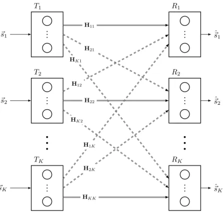
2.1 K-user MIMO Interference Channel. . . 9

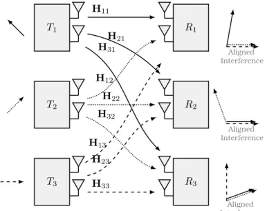
2.2 3-user MIMO Interference Channel when Interference Alignment (IA) is applied. . 10

2.3 Basic simulation scenario composed by a 3-cell cluster. . . 19

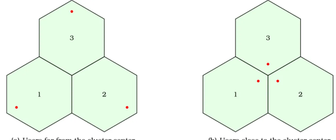
3.1 Simulation scenarios of channel imperfection analysis. Cluster with 3 cells with one mobile at each cell. . . 22

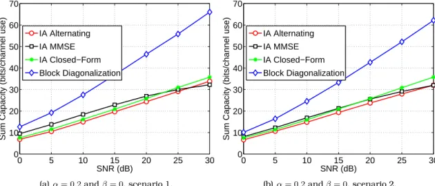
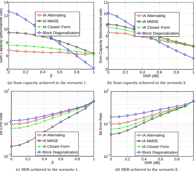
3.2 Sum Capacity as a function of the SNR for different combinations ofαandβ. . . 24

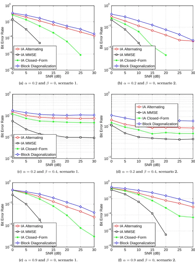
3.3 BER as a function of the SNR for different combinations ofαandβ. . . 25

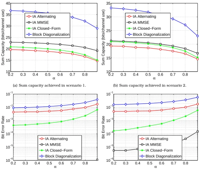
3.4 Impact ofαparameter on the algorithms performance for SNR= 15dB. . . 26

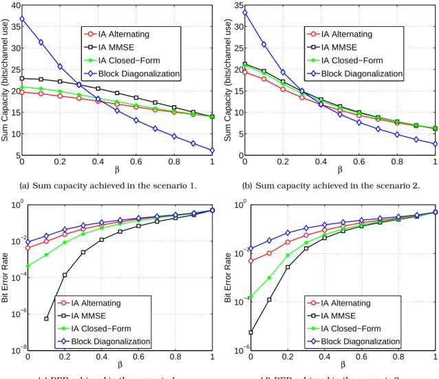
3.5 Impact ofβ parameter on the algorithms performance for SNR= 15dB. . . 27

3.6 Impact ofαparameter on the algorithms performance for SNR= 0dB. . . 28

3.7 Impact ofβ parameter on the algorithms performance for SNR= 0dB. . . 29

4.1 Receives inside the cluster perceiving an external interference, modeled as colored noise. . . 30

4.2 Simulation scenarios of external interference analysis. Cluster with 3 cells with one mobile at each cell. . . 34

4.3 Sum Capacity achieved by the algorithms versus External Interference level for different Signal to Noise Ratio (SNR) values at the border of the cell. . . 35

4.4 Sum Capacity versus SNR for different external interference values at the border of the cluster. At the left side, the results relate to the case in which users are distributed over all cells and at the right side, users are distributed respecting a distance of 2/3 of the cluster radius. . . 37

4.5 Bit Error Rate (BER) versus SNR for different external interference values at the border of the cluster. At the left side, the results relate to the case in which users are distributed over all cells and at the right side, users are distributed respecting a distance of 2/3 of the cluster radius. . . 38

4.6 Simulation with a Rank-1 external interference and nodes equipped with 4 antennas. The left side presents the Sum Capacity versus SNR while the right side presents the BER versus SNR, both for different external interference values at the border of the cluster. . . 41

4.7 Simulation with a Rank-2 external interference and nodes equipped with 4 antennas. The left side presents the Sum Capacity versus SNR while the right side presents the BER versus SNR, both for different external interference values at the border of the cluster. . . 42

(9)

4.8 Simulation with a Rank-4 external interference and nodes equipped with 4 antennas. The left side presents the Sum Capacity versus SNR while the right side presents the BER versus SNR, both for different external interference values at the border of the cluster. . . 43 4.9 Sum Capacity achieved by IA and BD algorithms as a function of the interference

level at the border of the cluster, with the external interference modeled with covariance matrices of different ranks. . . 44 4.10 Comparison of Sum Capacity achieved by IA, BD with users placed closer to the

edge of the cluster for different values of mobile speed. At the left side, the results concern the interference of 0 dBm at the cluster edge, while at the right side, the results are obtained considering 20 dBm of external interference. . . 48 4.11 Sum Capacity achieved by IA, BD with users placed closer to the edge of the

cluster for different values of external interference. At the left side the external interference was modeled with a rank-1 covariance matrix, while at the right side it was modeled with rank-4 covariance matrix. Considering the outdated channel with the solid lines and updated with dashed lines. . . 49 5.1 Multicell scenario composed by seven CoMP-cells. . . 51 5.2 CoMP-cell with its subregions for a hypothetic combination: core and periphery. 53 5.3 CoMP-cell with its subregions core and periphery for three different combinations. 53 5.4 Average throughput of the User Equipments (UEs) when each algorithm is applied. 55 5.5 Average throughput of the core UEs when each algorithm is applied for different

combinations of sectors performing the cooperation. . . 56 5.6 Average throughput of UEs when each algorithm is applied for different

combinations of sectors performing the cooperation. . . 57 5.7 Average throughput achieved by users in the core of the Coordinated Multi-Point

(CoMP) cell versus the load of the system for different schedulers and transmission schemes. . . 59

(10)

List of Tables

2.1 Simulation parameters of the 3-cell scenario . . . 19 4.1 Jakes’ channel parameters. . . 46 5.1 Simulation parameters of the multicell scenario. . . 51

(11)

List of Algorithms

2.1 Interference Alignment Closed-Form solution. . . 13 2.2 Interference Alignment via Alternating Minimization. . . 15 2.3 Interference Alignment with MMSE criterion. . . 17

(12)

Notation

Acronyms

3G ₃rd_Generation

3GPP ₃rd_{Generation Partnership Project} 4G _{4th Generation}

4-PSK _{4-Phase Shift Keying}

AWGN _{Additive White Gaussian Noise} BD _{Block Diagonalization}

BER _{Bit Error Rate} BS _{Base Station}

CoMP _{Coordinated Multi-Point} CPU _{Central Processing Unit} CSI _{Channel State Information} DoF _{Degree of Freedom}

FDD _{Frequency Division Duplexing} FDMA _{Frequency Division Multiple Access} FJP _{Full Joint Processing}

IC _{Interference Channel} JP _{Joint Processing} IA _{Interference Alignment} LAN _{Local Area Network} LTE _{Long Term Evolution} KKT _{Karush-Kuhn-Tucker}

MCS _{Modulation and Coding Scheme} MIMO _{Multiple Input Multiple Output}

MIMO-IC _{MIMO-Interference Channel}

MIMO-X _{MIMO-Cross Channel}

MMSE _{Minimum Mean Square Error} MSE _{Mean Square Error}

MRC _{Maximal Ratio Combining}

OFDMA _{Orthogonal Frequency Division Multiple Access}

PJP _{Partial Joint Processing} PSK _{Phase Shift Keying} PRB _{Physical Resource Block}

QAM _{Quadrature Amplitude Modulation}

(13)

QoS _{Quality of Service} SCM _{Spatial Channel Model} SER _{Symbol Error Rate} SNR _{Signal to Noise Ratio}

SINR _{Signal to Interference-plus-Noise Ratio}

SISO-IC _{SISO-Interference Channel}

SVD _{Singular Value Decomposition} TDMA _{Time Division Multiple Access} TP _{Transmission Point}

TTI _{Transmission Time Interval} UE _{User Equipment}

ZF _Zero-Forcing

(14)

Chapter

1

Introduction

1.1 Motivation

In the last decades the broadband services, bonded with multimedia applications, experienced a large growth and popularization. This increased the demand for very high data rates and Quality of Service (QoS). Associated to that, the people’s need to be connected every time and everywhere also increased. One of the keys to satisfy this necessity is through the employment of wireless communications systems, especially via the cellular based networks, since they allow the users’ mobility. In this context, these systems have undergone a fast expansion.

On another side, research on these communication networks has been focused on improving the transmission rates and creating systems with high spectral efficiency. Mainly guided by Shannon’s publication [1], that calculates the achievable channel capacity through some parameters of the systems, such as the transmission power and bandwidth. This chase for increasing the systems rate was intensified in the last decades. A good example is that the incoming 4th Generation (4G) systems must at least double the cell-edge throughput over the previous 3rd _{Generation (3G) networks [2]. Thus, seeking the performance improvement,} systems have changed their architecture, such as considering the Multiple Input Multiple Output (MIMO) approach.

However, a factor that has always limited the wireless communication systems performance is the interference. In these systems, all transmitters share the same medium to send the desired information to the receivers, which is an intrinsic wireless characteristic. Moreover, with the densification of these networks and the increasing demand for higher rates the importance of managing the interference has grown. Traditionally, the interference has been handled using basically three different approaches [3]:

i. Decoding the interference;

ii. Treating the interference as a noise;

iii. Interference avoidance.

(15)

1.2. State-of-the-art 2

methods limit the system performance. For the decoding case, there is a trade-off between improving the decode quality or the users’ data rate [3]. When the interference is neglected, it will clearly burden the data reception.

Nevertheless, the most common and important case of interference is when the interference has a similar strength to the desired signal. In this situation, the transmitters agree on transmitting through orthogonal resources, and in this manner the interference is avoided. So, a portion of the frequency or time, for instance, is divided among the neighboring transmitters, these methods are called Frequency Division Multiple Access (FDMA) and Time Division Multiple Access (TDMA), respectively. This method not only limits each transmitter performance but it also divides the available resources by the number of considered partitions. In order to reduce this performance loss, an approach similar to the frequency reuse can be applied, which performs the partition only for the closest transmitters [4]. However, this method may not be sufficient to provide the new throughput requirements, so, more refined techniques must be considered to handle the interference.

Therefore, combining the MIMO technology and the cooperation among the neighboring transmitters is a key to manage the interference and enable the system meet the required data rates. Aligned with this combination, the Coordinated Multi-Point (CoMP) architecture has been applied to achieve the aforementioned goals. One of the techniques that can be applied in this scenario is the Interference Alignment (IA), which is a novel method that claims that pairs of transmitters and receivers can perform transmissions free of interference and achieve the optimal multiplexing gain on MIMO systems [5]. Also, it was proven that by applying the IA technique, transmitters are able to send data with half of their channel capacity to his desired receiver, regardless of the number of users in aK-user Interference Channel (IC) network [6].

An example to perceive this gain is to consider the IC network composed by K pairs of transmitters and receivers. With a resource orthogonalization method, each pair is able to transmit at a rate equal to 1/K of the channel capacity. However, suppose that the medium adds a delay of one symbol duration to the interfering signals and two symbols to the desired signal. Then, if the transmitters send useful information and the receivers listen the channel just in the even time slots, then the communication of all pairs will become free of interference. This shows that in these networks, by applying a proper transmission method, the interference can be confined (aligned) in half of the dimension, remaining the other half to accomplish the transmissions free of interference. This, somehow, challenged the conventional wisdom about the throughput limits of wireless networks and made the technique arise as an important object of study in recent years. The following section briefly covers the state of the art in IA, but with no intention to exhaust the theme.

1.2 State-of-the-art

(16)

1.2. State-of-the-art 3

is just referred as IA.

The signal space alignment was introduced in [8], in which the impact of the interference on wireless networks was attempted to be characterized. This work showed that, when IA is applied, the achievable Degree of Freedom (DoF) of a MIMO-Cross Channel (MIMO-X) network, composed by two pairs of transmitters and receivers equipped with two antennas, are able to achieve four DoF, while the conventional methods achieve just three DoF. This gain could only be achieved by setting aside a part of the available dimension (time, frequency or space) at each receiver and forcing the interfering terms to be received in that partition.

Since this initial work, the interest on the characterization of other different networks via the DoF has increased, especially when the the IA technique is applied. Cadambe and Jafar (2008) [6] introduced the IA for the K-user IC with equal number of antennas at all transmitters and receivers, showing that this network can achieve up toK/2 DoF. Later this work was extend for an unequal number of antennas at each network node [9]. Similar IA schemes were proposed for X networks, where the useful signal is also transmitted in the crossed links for an arbitrary number of users [6].

Afterwards, some different algorithms were proposed to perform IA, some aiming at the perfect alignment, and others relaxing a little this constraint in order to obtain higher sum rates. The precoding design algorithm presented in [6] was extended to be accomplished in a distributed manner, and its convergence was proven in [10]. Results from these works established that these algorithms achieve the optimal Shannon capacity only at high Signal to Noise Ratios (SNRs) cases. In order to overcome this issue, an algorithm that tries to maximize the Signal to Interference-plus-Noise Ratio (SINR) instead of just performing the alignment was introduced in [11]. Both algorithms present a similar iterative framework, which enables them to find the appropriate precoder in different network configurations.

Still considering the objective of achieving the optimal gain on cases of finite SNRs values, an algorithm that minimizes the sum Mean Square Error (MSE) was introduced in [12]. By using the pricing concept, similarly as [13], these algorithms are also able to maximize several sum utilities, with different objectives, which enables the precoding design to follow a more egoistic approach (minimizing the interference that its own receiver perceives) or a more altruistic one (trying to avoid the interference that its transmitter causes on the unintended receivers). This precoding designing dilemma of compromising the beamforming gain at each intended receiver or mitigating the interference on the other receivers is also tackled in [14].

Several other works performed comparisons of the different proposed algorithms in several scenarios. The closed-form solution, an Minimum Mean Square Error (MMSE)-based algorithm, and another one that tries to minimize the interference that leaks at the receiver, had their performances compared within a two user X-network in [15]. The application of the technique in cellular networks was addressed by Suh and Tse (2008) [16] and by Sun, Liu, and Zhu (2010) [17], while [18] showed that IA almost doubles the throughput of MIMO Local Area Networks (LANs).

(17)

1.3. Open problems 4

increases. For instance, consider three transmitter-receiver pairs and let us assume each node is equipped with two antennas, then they can communicate with each other free of interference through IA. However, if the cooperation was performed with four pairs, the number of required antennas goes up to three, restricting the kind of devices that could be used.

At this point, IA has been shown to be a technique capable to mitigate the interference on several network configurations. Nevertheless, few works have approached the challenges of implementation in more realistic conditions. Most of the previous results on the literature were obtained considering ideal channels. One work that deviates from this focus is [20], which proposes an IA-based algorithm robust to Channel State Information (CSI) errors. The existence of an uncoordinated interference is considered in [21], however it limits itself to model the interference with just one dominant source.

The paper of Suh et. al. [2] is a relevant work that tackles some challenges of implementation, especially the extensive requirement of CSI to be exchanged over the network backhaul. Its main contribution was a new IA algorithm for downlink cellular systems that requires only intra-cell feedback. Furthermore, the work evaluates the proposed algorithms through a system level simulator that effectively performs the transmission between two cells while the surrounding cells are modeled as white Gaussian noise. This considered simulator could be improved, since even when IA is employed there is still uncoordinated interference, and more details are required for a more thorough systemic analysis. Nevertheless, the results of the paper aggregate relevant new information when compared with previous works.

Another work that tries to evaluate the technique in a more realistic scenario is [22], which analyzes some IA algorithms by using measurements of a real channel. Thus, by using the measurements, a 3-user frequency-selective SISO-Interference Channel (SISO-IC) is emulated, and the performance of IA schemes are compared with the method of interference avoidance that orthogonalizes the radio resource through frequency planning. This work provides pertinent results, however the presence of an external or uncoordinated interference can have a different impact on these two techniques, which is not taken into account in its isolated scenario.

Aiming to have a good picture of the IA technique behavior in real systems, recent works have focused on the system level performance evaluation. One example is the work that evaluates IA under different receive strategies through a 3rd _{Generation Partnership} Project (3GPP) compliant downlink Long Term Evolution (LTE) simulator [23]. The referred paper combines IA and other well established transmissions with a set of linear receivers, not worrying whether their design matches or not. For instance, the simulator can use the IA precoders with an Maximal Ratio Combining (MRC) reception, hence, in this case, the interference cancellation cannot be accomplished. This is a case in which the receivers are not able to perform complex computations.

Finally, it can be perceived that there are several research directions, but there are still some gaps on the discussed topics and some unresolved questions.

1.3 Open problems

Based on this brief review on the IA topic, it can be noticed that the research in this field has tackled different points and experienced a great advance. However several points are still unclear and deserve further investigations.

(18)

1.3. Open problems 5

those that proposed several precoding design algorithms, whose performances were evaluated basically in terms of the sum capacity, which translates the multiplexing gain, as well as the achievable DoF. Since the sum capacity achieved by the system is calculated just via the SINR perceived in each receiver, the transmissions are not effectively performed on the simulations of these works. Therefore, by simulating the transmission with different modulations and coding schemes the algorithms’ performances could also be analyzed through the Symbol Error Rate (SER) or Bit Error Rate (BER) results, which are metrics that can provide useful information on the reliability of the transmission links.

Besides IA, there exist other techniques that are able to mitigate the interference among cooperating transmitters. Most of them are based on the Joint Processing (JP) architecture, that requires coordination among all transmitters, which results on strong infrastructure requirements. In spite of this, these schemes are already considered on the new 4G networks. Therefore, another gap on the algorithms’ evaluation is that they have not been compared with other well-established techniques, such as the JP schemes.

Another issue on the evaluation of the technique is that the majority of the works considered perfect CSI knowledge at the transmitters to design the precoders. Nevertheless, there are basically two ways of gathering this information, namely by channel reciprocity and through feedback. The first one is based on the reciprocity principle that states that the transfer function of the direct channel (from transmitter to the receiver) at an instant is equal to the transpose of the reverse channel (from receiver to the transmitter). This is not valid, however, for Frequency Division Duplexing (FDD) systems, because these channels do not use the same frequency. The error can be minimized by using close frequencies in the downlink and in the uplink, but it cannot be avoided. The second manner is via feedback from the receivers, since they are able to easily estimate the channel. However the feedback transmissions are also susceptible to errors and delay, which may cause a significant impact on the final system performance. Thus, the consideration of perfect CSI knowledge for the precoding design may be not realistic.

On wireless communications, the obstacles are not equally distributed around the receivers, thus, the signal does not arrive from all directions, and some spatial directions may be enhanced. Also, at many receivers the space is insufficient to guarantee that the arriving signals are orthogonal at each antenna. Hence, another channel imperfection problem that was poorly addressed by past works is the correlation among antennas.

All the referred non-traditional methods to handle the interference require some kind of cooperation to mitigate it. Also, with the growth of the number of wireless systems, it can be difficult to employ such cooperation among a large number of transmitters. Hence, it is common to have coexisting networks that interfere with each other. Therefore, the consideration of the presence of an external interference is another realistic assumption, which was tackled in [2, 21]. However, due to the rather simple models that were used, there are some further unresolved issues in this topic.

(19)

1.4. Objectives and contributions 6

1.4 Objectives and contributions

The last two sections addressed the already studied and some unresolved issues on the IA topic. Thus, this work aims to provide useful evaluations of some algorithms, seeking to clarify how the technique will work in practical systems.

For this work, the cellular network is adopted as the main scenario where the IA algorithms will be employed and assessed. So, the first contribution of this work is the evaluation of the IA technique in this scenario. However, this evaluation is taken not just in terms of the sum capacity achieved by the system, but also through the BER results. Also, the comparison with one JP-based transmission scheme is accomplished, in order to better understand the actual gain that the technique could provide. In this manner, the assessment of the algorithms is not limited to the theoretical gains and it could provide more useful insights into how the IA technique could really perform in practice.

Therefore, aiming to go a step further on the comprehension of how realistic conditions will affect the technique’s performance, some channel imperfections are added in the simulator. First, an additive error in the CSI is considered for the precoding design. Then, correlation among the transmitter antennas is assumed. The JP-based transmission scheme is also compared with the IA algorithms.

Parallel to that, the presence of an uncoordinated interference is considered in the same simulator. This interference is modeled as a colored noise, and the rank of its covariance matrix is changed to mimic different kinds of interference. If there is just one dominant interference, the rank of the covariance matrix must be one, if there are two the rank must be two, and so on. This model can embrace several kinds of interference. In this scenario, some changes were made to the IA algorithm in order to take into account this external interference. Also, a modification of one IA algorithm is proposed, in order to try a better alignment of the internal and external interference. As a matter of fairness, the JP-based algorithm is also modified to account for the uncoordinated interference at the precoding design.

In order to also evaluate the impact of temporal channel variations on the IA technique, the channel is generated using the Jakes’ model, which allows to assess the impact of the delayed channel on the algorithms’ performances. So, this channel imperfection and the uncoordinated interference can be combined in this set of simulations.

Although the previous analyses tackle some important factors that are present in real systems, the analysis was performed at a not too realistic scenario, assuming a simulated system composed of just three transmitters, while in practice this number is much larger. Furthermore, the transmission considered only one modulation scheme and no coding. For the purpose of assessing IA in a scenario closer to practice, this work additionally performs system level simulations in a larger network. In this scenario, not only the IA algorithms are compared but some schedulers are evaluated as well.

1.5 Outline

After briefly presenting the current context of Interference Alignment research, this dissertation is further divided into five chapters, whose contents are as follows:

(20)

1.5. Outline 7

is analyzed. So, it starts by presenting the model of the additive error in the CSI and the correlation among transmission antennas. It finishes by presenting the analyses of the simulations results;

◮ _{Chapter 4}_{: The analyses of how the external interference affects the IA algorithms are} performed in this chapter, so, the model of the uncoordinated interference is shown and some algorithms’ modifications are presented. The channel variations are also considered in this chapter, then the Jakes’ model is discussed and the impact of the delayed channel knowledge is studied here;

◮ _{Chapter 5}_{: The IA technique evaluation ends in this chapter by performing the} assessment in a system level simulator. Similar to the previous analysis the IA algorithms are compared with JP-schemes of transmission in a more elaborated simulator. In this simulator, some scheduling policies are also evaluated.

(21)

Chapter

2

Interference Alignment

This chapter begins presenting the system model used through almost all the work. From this system model the basic concepts of Interference Alignment (IA) are discussed, followed by the presentation of the algorithms based on the technique. And the chapter is closed by showing the simulator framework used in the forthcoming analysis.

2.1 System Model

The MIMO-Interference Channel (MIMO-IC) is composed by a set of transmitters and receivers that are organized in pairs, meaning that each transmitter desires to send information to its respective receiver, as illustrated in Figure 2.1. Thus, the interference is composed by the union of all signals arriving at the receivers that were not sent by their correspondent transmitter. This model can perfectly emulate the scenario chosen to evaluate the IA technique, a cellular network, since there is a link between each user and Base Stations (BSs).

So, hereafter theK-User MIMO-IC network is considered, where each of theKtransmitters is equipped with NT antennas and wants to send S streams to a specific receiver that is

equipped withNRantennas. Then, data is precoded and transmitted, resulting in the following

received signal:

yk=HkkVkdk+ K X

j=1,j6=k

HkjVjdj+nk, (2.1)

whereHkj ∈ CNR×NT denotes the channel between transmitterj and receiver k, Vk ∈CNT×S

and dk ∈ CS×1 denote, respectively, the precoder and the vector of symbols of the k-th

transmitter, finally,nk ∈CNR×1 is the white Gaussian noise vector with varianceσn2. In order

to recover the original data streams, the received signalyk ∈CNR×1 is processed by applying

the receive filterUH

k ∈CS×NR at the receiver side.

Given the system variables, the Signal to Interference-plus-Noise Ratio (SINR) of thej-th stream of thek-th user in the network is given by:

SINR=γ_k[j]= |u [j]H

k Hkkv

[j]

k |2 S

P d=1

K P i=1|

u_k[d]HHkiv_i[d]_|2_{− |}_u[j]H

k Hkkv

[j]

k |2+||u

[j]H k ||2σ2n

, (2.2)

(22)

2.2. Interference Alignment Concept 9

.. .

T1

~s1

.. .

T2

~s2

.. .

TK

~sK

.. .

R1

ˆ

~s1

.. .

R2

ˆ

~s2

.. .

RK

ˆ

~sK

H11

H21

HK1

H22 H12

HK2

HKK

H2K

H1K

..

.

..

.

Figure 2.1:K-user MIMO Interference Channel.

2.2 Interference Alignment Concept

The main idea behind this novel technique is to align, at each receiver, multiple interference signals in a subspace with dimension smaller than the number of interferers [2]. This is a very general idea, in the sense that the signals can be aligned in any dimension, including time, frequency, or space. Also, it can be viewed as a cooperative and altruistic approach since the transmitters may neglect the performance of their own link to allow other users to perfectly cancel interference [21].

Thus, what the IA technique does is to design the precoders and the receiver filters so that the interference can be canceled at every receiver. Hence, the generic IA problem can be written as:

UH_kHkjVj= 0,∀j6=k (2.3)

rank UH_kHkkVk=S. (2.4)

Note that a space of dimension S is required to confine the interference at each receiver. Nevertheless the analytical solution of this system of equations is known for just a few scenarios. In the following two very important concepts are addressed, which help to understand how the technique works and its possibles gains.

2.2.1 Degree of Freedom

In the context of communication networks, capacity is a measurement of the maximum amount of data that may be transferred on the network. The exact capacity for most wireless networks is unknown, thus, the best way to assess the capacity limit is through approximations. Specifically, for a single Multiple Input Multiple Output (MIMO) transmitter-receiver pair, it can be described as a function of the Signal to Noise Ratio (SNR) as:

(23)

whereηis called multiplexing gain, which represents the number of streams that can be sent in (almost) parallel channels. In [5] it was shown that this gain can achieve, with the right processing, a multiplexing gain equal to the minimum between the number of transmit and receive antennas.

The termo(log(SN R))becomes negligible at high SNR in relation to thelog(SN R), thus the following relation can be defined:

η, _lim

SNR→∞

C(SNR)

log(SNR), (2.6)

which represents the ratio between the linear scale of the capacity and the logarithm of the SNR. For the multiuser case this increasing factor is called Degree of Freedom (DoF). When a network presents such behavior it is common to say that it achieved the optimal multiplexing gain.

This concept was the main study object of the first IA works, and before them it was shown that a fully connected K-user Interference Channel (IC) network achieves only one DoF [6]. However, by applying the IA technique, K/2 DoF can be reached. Therefore, most works focused on finding the achievable DoF of several network configurations, which made this concept very important on IA studies. Consequently, it is worth to highlight three points of view about this concept:

i. A network hasηdegrees of freedom if and only if the sum capacity of the network can be expressed asηlogSNR+o(logSNR);

ii. It provides a good capacity approximation at the high SNR regime;

iii. The degrees of freedom of a network may be interpreted as the number of resolvable (interference-free) signal space dimensions.

This last interpretation is illustrated by the example exposed in Figure 2.2, which shows the application of IA in a 3-user MIMO-IC network. In this example, the interferences signals are aligned in one direction, at each receiver. Therefore, each user has one dimension free of interference for the transmission of the desired signal. Thus, it is said that this system can achieve3/2DoFs.

T1

T2

T3

R1

R2

R3

H11

H21 H31

H22 H12

H32

H33 H13

H23

Aligned Interference

(24)

2.2.2 Feasibility

From the DoF concept, lots of works derived the theoretical gains that IA could provide on different kinds of networks. However, the technique cannot be randomly applied in a network and expect that the interference will be completely eliminated. There are some conditions regarding the configurations (number of antennas, streams transmitted, etc.) that must be respected. As an example, considering IA along the spatial domain, as the number of cooperating transmitters increases, the number of antennas required to accomplish the alignment also increases. In this regard, the relation between the number of users, antennas and transmitted streams was derived in [19], which is referred to as the feasibility conditions to achieve IA. These conditions play an important role on the choice of scenario to which the technique can be applied.

From the generic IA problem in (2.3), it can be perceived that the interference is eliminated by choosing the right precoders and receiver filters, through the solution of the system of equations. These systems can present one solution, infinite solutions and no consistent solution, but how they are classified depends on the number of variables and equations involved. If there are more independent equations than variables, the system has one or more solutions. So, to know if the IA problem has any solution it is just necessary to count the number of independent equations and variables involved. These numbers are intrinsically dependent on the configuration of the network, how many antennas each node is equipped with, how many pairs are cooperating to accomplish the alignment and etc. Then, in order to determine for each scenario whether the IA algorithms could be applied, the number of equations and variables are accounted for as follows.

Considering the system model adopted in this work, both the equations and variables involved in the system can be counted. Thus, in order to know the number of equations that effectively participate of the solution, the IA problem can be rewritten as:

u[_km]HHkjv[_jn] = 0,_∀j₆=k and_∀m, n_{∈ {}1,2,_{· · ·} , S_} (2.7)

wherev[_jn] andu_j[n] are then-th column of thej-th precoder and receive filter, respectively. Consequently, assuming that each user has the same number of streams si = S, the

number of equations present in the system is:

Ne=

K X

j,k=1

j6=k

sisj =

K X

j,k=1

j6=k

S2= (K2₋K)S2. (2.8)

Counting the number of variables is not as direct as the number of equations. Some of the variables are not useful on the solution of the problem and it is necessary to be careful not to include them into the count. For instance, considering the transmitterk that applies the Vk∈CNT×S precoder, the first thought is to consider its dimension as the number of variables.

However, consider a square matrixB, obtained from removing theNT −S last lines of theVk

matrix. Then, the vector space generated byVkBis the same spanned by Vk. Consequently,

there are onlyNT−Suseful variables in each precoding filter. If the same process was applied,

then the same conclusion can be taken for the receiver filter, thus onlyNR−Suseful variables

(25)

2.3. Interference Alignment Algorithms 12

is given by:

Nv=

K X

i=1

si(NT +NR−2si) =

K X

i=1

S(NT+NR−2S) =KS(NT+NR−2S). (2.9)

Finally, in order to know if the network configuration is feasible for the IA technique, considering a symmetric system, the number of variables has to be equal or greater than the number of equations. Thus, the following rule can be derived:

NT +NR−(K+ 1)S≥0 (2.10)

The most analyzed configuration is the 3-user channel, where the nodes are equipped with two or four MIMO antennas. Considering the 2_×2 case, the feasibility rule in (2.10) will show that each user is able to send just one stream. Also, this rule shows that if four users are considered then two antennas per node are not sufficient to solve the IA problem. If the number of antennas is increased by two, i.e. 4_×4 case, the number of streams each user is able to send increases just by one. So, this shows that, as the number of interferers increases, the number of antennas required to perform the technique grows faster, which can be a problem for the technique.

2.3 Interference Alignment Algorithms

This section presents the algorithms based on IA that will be evaluated in this work. All of them enable the network to achieve the previously mentioned DoF if the feasibility conditions are respected. Also, the first two algorithms aim at the perfect/pure interference alignment, while the last one relaxes this constraint in order to improve the direct channel.

2.3.1 Closed-Form Solution

The first algorithm presented here is the IA closed-form solution for the 3-user case of MIMO-IC. This algorithm can be very useful for the comprehension of the IA concept, since the alignment can be seen in a more explicit way than in the other algorithms. The 3-user case solution is calculated by solving the following system of equations, that represents the alignment of the interfering signals at each receiver:

span(H12V2) =span(H13V3), (2.11) span(H21V1) =span(H23V3), (2.12) span(H32V2) =span(H31V1), (2.13)

where span(A)corresponds to the subspace generated by the columns ofA. These conditions can be even more restrictive when rewritten as:

span(H12V2) =span(H13V3), (2.14)

H32V2=H31V1, (2.15)

(26)

So, ifV2andV3were written as function ofV1, then the system is given by:

span(H12H−321H31V1) =span(H13H−231H21V1), (2.17) V2=H−321H31V1, (2.18) V3=H−231H21V1. (2.19) Then, the solution forV1is any subset ofS eigenvectors of the following matrix:

E=H−₃₁1H32H₁₂−1H13H−₂₃1H21. (2.20) This way there are CS

2S = ₂_S

S

ways to choose the precoder of the first transmitter, and all of the solutions accomplish the perfect interference alignment at each receiver. It turns out that this precoding design guarantees that the interference is aligned for each user. Hence, in order to completely eliminate the interference and revert the channel effect, then a Zero-Forcing (ZF) receiving filter may be applied at each receiver. Therefore, the receiver matrices must be calculated respecting the following relation:

UH₁[H12V2 H13V3] = 0, UH₂[H21V1 H23V3] = 0, UH₃[H31V1 H32V2] = 0,

(2.21)

since the precoders already aligned the interferences, then the relation becomes:

UH₁[H12V2] = 0, UH₂[H21V1] = 0, UH₃[H31V1] = 0.

(2.22)

Note that the direct channels are never used in this algorithm, and thus how much the direct signal lies inside the null space cannot be controlled. Also, if a different subset of precoders are chosen, then the algorithm may perform differently. So, each different subset of the eigenvectors ofE yields a distinct IA solution. Hence, in order to boost the closed-form solution performance, the set of precoders that maximizes the minimum of the SINRs may be used. For a reasonable number of antennas (e.g. , 2 or 4), performing this choice is not too costly, since the exhaustive search will be done among two or four choices. This algorithm is labeled as IA closed-form strategy and it is summarized in Algorithm 2.1.

Algorithm 2.1Interference Alignment Closed-Form solution.

i. Using (2.20) calculate theEmatrix;

ii. AssignS eigenvectors ofEforV1;

iii. Use (2.18) and (2.19) to obtainV2 andV3;

iv. Calculate the receiver matrices of each user,UH

k , according to (2.22) .

2.3.2 Interference Alignment via Alternating Minimization

(27)

in [6] and presents a lot of advantages over the closed-form solution. First, it can be applied to several network configurations, as long as the feasibility conditions are respected, which provides more flexibility to the technique. Also, it can be performed in a distributed manner, i.e., it is not necessary to have a Central Processing Unit (CPU) where all the estimates of the network are concentrated to design the precoders. So, this is an indispensable algorithm to the analyses performed in this work.

The IA via alternating minimization is not accomplished by directly solving that system of equations. It is based on the concept of subspaces, for which the available dimension at each receiver can be split in two subspaces. The first one is where the desired signal is decoded and the other is where the interference must be confined. Thus, what this algorithms makes is to adapt the interference subspaces and the precoders to accomplish the interference alignment. Thus, considering this subspace approach, the function that translates the IA objective and must be minimized is:

JIA=

K X k=1 E Φ H k K X

j=1,j6=k

HkiVisi 2 F . (2.23)

whereΦk is an orthonormal basis for the interference subspace.

Considering the independence of the signals, the instantaneous objective function is:

JIA=

K X k=1 K X j=1

j6=k

tr ΦH_k HkjVjVHj HHkjΦk, (2.24)

which can be seen as the power of the leaked interference. Also, the precoders must satisfy the power constraints.

This function can be minimized through an alternating optimization approach, by choosing the precoders and interference subspace as:

Φopt_k =νSmin     K X j=1

j6=k

HkjVjVHj HHkj   

, (2.25)

and

Vopt_k =νminS     K X j=1

j6=k

HH_kjΦjΦHj Hkj   

, (2.26)

where ν(_·)S

min is a function that returns a matrix whose columns are the eigenvectors

corresponding to theS smallest eigenvalues of the input matrix.

Translating into words, at the first step, users try to adapt their interference subspace towards the direction of interference caused by the other transmitters. On the second step, by knowing the subspaces of all users, each transmitter tries to change its precoder to project, onto these subspaces, the interference caused at the other users. Thus, these two steps are alternately performed until the algorithm converges. Convergence that can be proved by showing that at each iteration the objective function decreases. It is important to remember that although the convergence to a minimum can be proved, the interference alignment is just accomplished when the feasibility conditions are respected.

(28)

that the initial precoders can be randomly initialized. It is important to highlight that a maximum number of 60 iterations is considered for the simulations, which was verified to be almost always enough to provide good alignment in the 3-user case, while for 5 or 7-user scenarios 260 and 800 iterations are required, respectively.

Algorithm 2.2Interference Alignment via Alternating Minimization.

i. Initialize the set of precoders;

ii. Find the interference subspace, PK

j=1,j6=k

HkjVjVHj HHkj, of each user;

iii. Assign the orthonormal basis of the interference subspace as the S dominant eigenvectors of the interference subspace, according to (2.25);

iv. Calculate PK

j=1,j6=k

HH

kjΦjΦHj Hkj for each user;

v. Assign the precoders as the S dominant eigenvectors of the matrix calculated in the previous step, according to (2.26);

vi. Repeat from stepiiuntil convergence.

Besides the already mentioned flexibility of this algorithm, another interesting feature is that it provides orthogonal precoders, which are especially attractive when the Channel State Information (CSI) is quantized.

2.3.3 IA-MMSE

In order to have a broader picture of the IA technique, here an IA algorithm that uses the Minimum Mean Square Error (MMSE) criterion at the reception is presented. Its solution tries to balance the goals of aligning and eliminating the interference at the receivers with the need of keeping the signal level well above the circuit noise [21]. Similar to the IA alternating algorithm, the IA MMSE uses an alternating optimization framework to find the precoders and receive filters. Also, the MMSE approach is flexible in the same manner of the alternating algorithm, and it must still satisfy the feasibility conditions.

The MMSE criterion seeks to minimize the error in the reception, thus, the Mean Square Error (MSE) is related to the difference between the decoded and transmitted symbols, which can be written as:

MSEk = K X

k=1

E_kUH_k yk−dkk2. (2.27)

Replacing the received signalyk from (2.1) in (2.27) yields:

MSEk = K X k=1 E U H k 

HkkVkdk+ K X

j=1,j6=k

HkjVjdj+nk  ₋dk

2 . (2.28)

Hence the MMSE optimization problem to be solved is given by:

min

{Vk};{Uk}

K X

k=1 tr

 UH_k

 

K X

j=1

HkjVjVHj HHkj+σkI  Uk



₋2R_tr UH_k HkkVk (2.29)

subject to tr(VHj Vj)≤Pj; ∀j={1, . . . , L}, (2.30)

whereR_{·}corresponds to the real part of a number.

(29)

to find a solution. The Lagrangian of this optimization problem is written as:

L₌

K X

k=1 tr

 UH_k

 

K X

j=1

HkjVjVHj HHkj+σkI  Uk



₋2R_tr UH_k HkkVk

+

K X

j=1

µj tr VHj Vj−Pj,

(2.31)

where µj is the Lagrangian multiplier for the precoder j. Hence, the Karush-Kuhn-Tucker

(KKT) conditions are:

∇L₌₀ (2.32a)

µj tr VjHVj−Pj= 0, ∀j (2.32b)

tr V_jHVj≤Pj, ∀j (2.32c)

µj≥0,∀j (2.32d)

In order to solve this problem, it is assumed that the set of precodersVj is initially fixed

andµj ≥0, which satisfies the KKT conditions (2.32b)-(2.32d). The gradient of the receiver

filter,Uk, can be calculated from the first KKT condition, resulting in:

Uk =  

K X

j=1

HkjVjVHj HHkj+σn2I  

−1

HkkVk. (2.33)

Likewise, fixing the receive filters allows the derivation of the precoders from the first KKT condition. The precoderVj is then given by

Vj= K X

k=1

HH_kjUH_kUkHkj+µjI !−1

HH_jjUH_j . (2.34)

However, unlike the receive filters, the other KKT conditions are not automatically satisfied. Hence, the equality and inequality cases in (2.32d) must be checked. First, ifµj = 0, then

the other conditions are satisfied and the optimal precoder is directly found from (2.34). If µj > 0, it implicates that tr VHj Vj = Pj, and the Lagrange multipliers µj must be found.

Unfortunately, even ifVj were replaced from (2.34) in (2.32b), a closed form solution for µj

cannot be found. On the other hand, it can be observed that the power of the precoder is monotonically decreasing as a function of the Lagrangian multiplier. Therefore, the bisection method can be applied to find the Lagrange multiplier and finally calculate the precoder from (2.34).

Note that, similarly to the Alternating Minimization algorithm in Section 2.3.2, this non-trivial coupled optimization problem can be solved by an iterative framework where a set of variables are fixed while the other one is calculated, repeating the process for each variable. The MMSE-based IA algorithm is summarized in Algorithm 2.3.

It is expected that the MMSE-based algorithm outperform the Alternating Minimization algorithm, since it accounts for the impact of the thermal noise. On the other hand, the IA MMSE algorithm does not provide orthogonal precoders as the Alternating Minimization algorithm. Moreover, the MMSE-based algorithm is much more complex because it requires solving two optimization problems at every iteration.

(30)

2.4. Block Diagonalization 17

Algorithm 2.3Interference Alignment with MMSE criterion.

i. Initialize the precoder matricesVj with the closed-form solution; ii. Calculate the receive vectors,Uk ,using (2.33);

iii. Solve µj by replacing (2.34) on the power constraint of transmitter j, then update Vj

according to (2.34) with solvedµj; iv. Repeat from stepiiuntil convergence.

the precoder is fixed, then the received filter is calculated and vice-versa. At each iteration the MSE always decreases, which ensures that the algorithm will converge to at least a local minimum. Some preliminary simulations were performed and the IA MMSE algorithm achieves a very good performance with only 32 iterations, assuming it is initialized with the closed-form solution.

This initialization method has a large impact on the complexity of the algorithm, since if the precoders are randomly initialized, the algorithm needs more than 100 iterations to converge. On the other hand, this initialization can be performed just for the three-user case, since the closed-form solution is only known for this case. Also, the distributed manner that this algorithm may be applied is no longer possible.

2.4 Block Diagonalization

Previously, the algorithm discussion was started by describing the closed-form solution of IA, which is the purest form to achieve the interference alignment goal. Then, a more flexible algorithm was introduced that can be implemented in a distributed form. Finally, the IA goal is relaxed and an MMSE-based algorithm is applied. All these three algorithms cover some relevant issues regarding wireless networks, and assessing them could provide some insights on the IA performance. Nevertheless, with the purpose of grasping how good the IA technique can perform, it is still necessary to have a benchmark for them.

On current cellular networks, Joint Processing (JP)-based transmission schemes are already considered. These schemes presume a cooperation among the transmitters to avoid the interference, similarly to the IA technique. However, they require not only the information about the channel matrices of the network, but they also need the knowledge of all the data that will be sent at each transmitter. This demands much more from the infrastructure than the IA technique. Hence, it is most likely that these schemes are able to achieve better performance than IA, which can be considered as a goal for IA performance.

At the JP-based schemes there is cooperation among the different transmitters, where each one participates on the transmission of all users of the network. Then the network can be treated as if there were just a single virtual MIMO transmitter. So, as all transmitters will send useful information to all receivers, the channel model shown in Section 2.1 can be rewritten as:

yk = K X

j=1

HkMjdj+nk

=HkMkdk+ K X

j=1,j6=k

HkMjdj

| {z }

Interference

+nk,

(2.35)

where Hk = [Hk1 Hk2 · · · HkK] is the matrix comprised by concatenation of the channel

matrices of all transmitters to the desired userk. AndMkis the modulation matrix associated

(31)

2.4. Block Diagonalization 18

Diagonalization (BD) [24].

Accordingly, the block diagonalization process is accomplished with a cascade of two precoding matrices,Bk, that removes the intra-cell interference, andDk, which is responsible

for parallelizing the transmission. Hence, the block diagonalization precoding matrix is Mk=BkDk.

The first step to accomplish Block Diagonalization is to eliminate all multi-user interference, hence the constraint HkMj = 0 for k 6= j is imposed. This means that the

interference parcel of (2.35) will be forced to zero. Thus, consider the matrixHke , formed by the concatenation of the interfering channel matrices, that spans the interference subspace of userkand is written as:

e

Hk= [H1· · ·Hk−1 Hk+1· · ·HK]. (2.36)

and its Singular Value Decomposition (SVD) is defined as:

e

Hk =Uek h

e

Λk 0 i h

e

V(1)_k Ve_k(0)iH, (2.37)

then,Bk is constructed by choosing theLk columns of Ve(0)k , which form the orthogonal basis

for the right null space of Hke . This will automatically eliminate the interference, and the received signal is resumed to:

yk=HkBkDkdk+nk. (2.38)

It is worth to highlight that for the network configuration used in this work, that is composed by pairs of transmitters and receivers equipped with equal number of antennas, the nullity of theHek matrix isNR, assuming the linearly independence of the channels. This

results in a null space of dimension ofLk =NR, which corresponds to the number of available

dimensions to parallelize the streams transmission. In the 3-user case, with two antennas per node, this algorithm allows each pair to send two streams free of interference, while IA is able to send just one. This gain over IA is explained by the full coordination performed by the BD algorithm. Furthermore, in the following analysis it is expected that in terms of sum capacity this algorithms could be seen as an upper bound.

Now the data streams must be parallelized, which can be performed through another SVD. Consider the definition ofHef f,k as:

Hef f,k=HkBk=UkΛkVHk , (2.39)

then the parallelize precoder matrix can be chosen as Vk and the decoder will be UHk . To

obtain an optimum transmission, theVk matrix can be scaled with a power control matrix,

P12

k, that can be calculated through the water-filling algorithm with the singular valuesΛk.

This whole process on designing the preceoders can be summarized as:

Mk=BkDk=

e

V(0)_k (1:Lk)

VkP 1 2

k. (2.40)

and the reception is performed just by the application of theUH_k matrix.

(32)

2.5. Simulation framework 19

2.5 Simulation framework

First it is important to highlight that the simulation scenarios of this work are always based on cellular networks. So, in order to emulate the current networks, here the2_×2and 4_×4 MIMO antenna configurations are considered. It should be mentioned that, currently, the4×4MIMO antenna configuration can be seen as a baseline while the8×8MIMO antenna configuration is the maximum accepted for special systems [25]. Moreover, at the2_×2MIMO case IA is able to handle only three cooperative transmitters (see Section 2.2.2). Since the BD algorithm will also be employed, the simulation framework is composed by a Coordinated Multi-Point (CoMP) cluster composed by three cells, shown in Figure 4.2.

1 2

3

Figure 2.3:Basic simulation scenario composed by a 3-cell cluster.

At this CoMP cluster, there is a BS placed in the center of each cell. Furthermore, each cell contains a receiver/user, that can be placed respecting different distributions. The transmission power available to the transmission of each BS is calculated in order to match a specific value of SNR at the border of the cell. Thus, the location of the users and the SNR parameter can be varied in order to provide different SINR cases. The transmissions are performed using the 4-Phase Shift Keying (4-PSK) modulation scheme with no codification. Finally, a summary of the common parameters used in the simulations are highlighted in Table 2.1

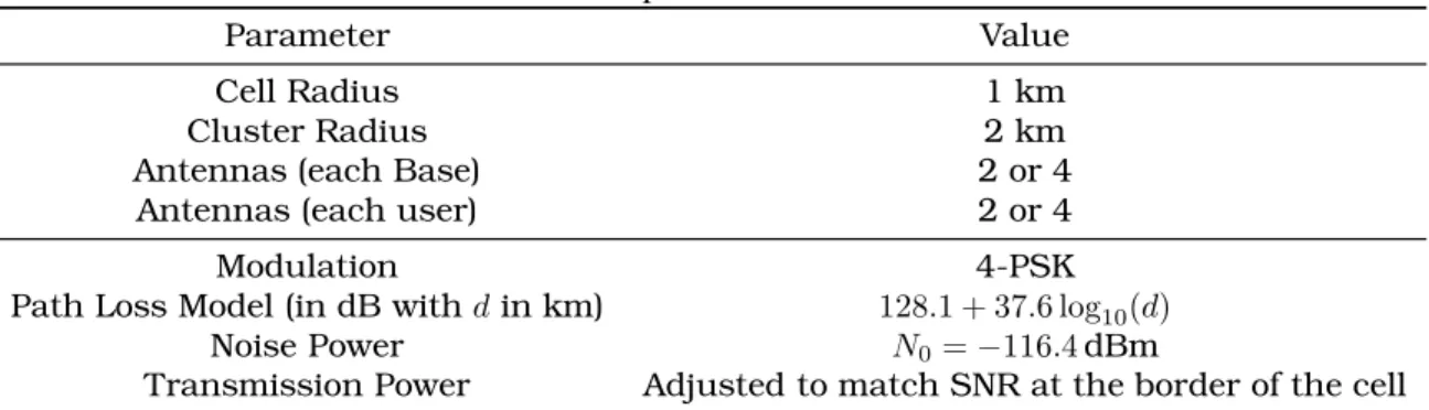
Table 2.1:Simulation parameters of the 3-cell scenario

Parameter Value

Cell Radius 1 km

Cluster Radius 2 km

Antennas (each Base) 2 or 4

Antennas (each user) 2 or 4

Modulation 4-PSK

Path Loss Model (in dB withdin km) 128.1 + 37.6 log10(d)

Noise Power N0=−116.4dBm

Transmission Power Adjusted to match SNR at the border of the cell Since this is a CoMP cluster, it is assumed that there is a fast backhaul that enables the data exchange among the base stations. It is important to remember that some IA algorithms, such as the IA Alternating, can be performed on distributed architectures, while others, like the Closed-Form solution, require a CPU. This architecture analysis is left for future work and it is considered that all transmitters have the estimates required to calculate the precoders and receiver matrices, unless otherwise stated. Regarding the external interference, its model is left to be presented in chapter Chapter 4.

(33)

2.5. Simulation framework 20

average Bit Error Rate (BER) achieved by the system can be computed in order to grasp the error robustness of the algorithms. Complementary to that, a metric that can translate the maximum rate that the system can achieve is the sum capacity. The SINR of each stream decoded at each receiver can be calculated by (2.2), and then the capacity formula can be applied:

C= log2(1 +SIN R). (2.41)

(34)

Chapter

3

Channel Imperfection Analysis

This chapter begins the performance evaluation and the comparison of the previously presented algorithms. Moreover, two kinds of channel imperfection are considered in order to emulate a more realistic scenario. Thus, the influence of correlation between the transmitter antennas and the assumption of imperfect Channel State Information (CSI) knowledge are included on the modeling of the channel coefficients. Next section presents how these imperfections were modeled in this dissertation.

3.1 Imperfection Models

The channel model applied to simulate the correlation among antennas is the Kronecker channel model, which has a simple analytic treatment [26]. The characterization of this model separates the correlation at the transmission and at the reception, which is a quality that fits well with this work’s purpose. Then, the Multiple Input Multiple Output (MIMO) channel from transmitterj to receiverkis modeled as:

Hkj =

1

p

tr{Rr}

R_r1/2Hw_kjR_t1/2T _∀j, k_{∈ {}1, . . . , K_}, (3.1)

whereHw_kj _{∼ CN}(0,I). The receive and transmit correlation matrices are denoted by Rr and

Rt, respectively. The correlation at the reception is not considered here, then the receive

correlation matrix is assumed to be an identity matrix. The transmit correlation matrix has its elements calculated from a single parameterα, and is given by [27]:

Rt(m, n) =|α||m−n| form, n∈ {1, . . . , NT}, (3.2)

whereNT is the number of transmit antennas. This model is widely used in the literature and

industry and represents the correlation between elements of a uniform linear antenna array, whereα= 0and_|α_|= 1correspond to no correlation and rank 1 channel, respectively [28].

For the imperfect channel modeling, it simply considered the addition of noise to the actual channel matrices. Thus, the channel matrices used at the precoding design stage will be given by [28]:

Hw_kj =p1−β2_H˜w

kj+βEkj, (3.3)

(35)

3.2. Channel Imperfection Results 22

varying from zero to one. That is,β = 0corresponds to perfect channel knowledge and β = 1 corresponds to no CSI knowledge at the transmitter.

When taking both channel correlation and CSI error into account, the full channel model is then given by

Hw_kj=p1₋β2_H˜w

kj +βEkj

·R1_t/2. (3.4)

3.2 Channel Imperfection Results

In order to assess the impact of channel imperfections on the performance of the Interference Alignment (IA) algorithms, two variations were considered on the cellular network scenario first presented in Section 2.5. These variations were chosen to provide cases on which the receivers do not perceive too much interference from the unintended transmitters and the other case where this interference is much stronger. Thus, in the first case the three users are placed far from each other respecting a distance of 70% of the cell radius from its respective transmitter, as shown in Figure 3.1(a). In the other case, illustrated in Figure 3.1(b), the users are near to each other respecting the same distance to the center of the cell, so that the pathloss that users experiment in both cases is the same. It is important to say that in this analysis the nodes are equipped with two antennas, hence, when they are employing IA algorithms, each transmitter-receiver pair sends one stream. However, when the Block Diagonalization (BD) scheme is employed the pairs are able to send two streams each.

1 2

3

(a) Users far from the cluster center.

1 2

3

(b) Users close to the cluster center.

Figure 3.1:Simulation scenarios of channel imperfection analysis. Cluster with 3 cells with one mobile at each cell.

The algorithm comparison starts by showing how their performance, in terms of the sum capacity, behaves when the Signal to Noise Ratio (SNR) is varied, under different cases of channel imperfections. Figures 3.2(a) and 3.2(b) present these performances when the CSI is perfectly known,β= 0and the correlation among the antennas is very weak,α= 0.2. First, all the algorithms present an almost linear gain with the scaling of the SNR, on both scenarios, which means that all of them were able to mitigate the interference and are just limited by noise. As expected, the BD algorithm achieves the highest sum capacity, at both scenarios, since it can send more streams than the IA-based schemes. Regarding the comparison among the IA algorithms, it can be perceived that those that apply the Zero-Forcing (ZF) filter at the reception, IA closed-form and IA alternating, present a slightly worse performance than the IA Minimum Mean Square Error (MMSE), this happens because their objective is just to accomplish the interference alignment, they do not care about the direct channel. Also, the IA closed-form is better than the alternating due to the choice of the best set of precoders.