FEDERAL UNIVERSITY OF CEARÁ
DEPARTAMENT OF TELEINFORMATICS ENGINEERING
POSTGRADUATE PROGRAM IN TELEINFORMATICS ENGINEERING
MARCIEL BARROS PEREIRA
PARTICLE SWARM OPTIMIZATION AND DIFFERENTIAL
EVOLUTION FOR BASE STATION PLACEMENT WITH
MULTI-OBJECTIVE REQUIREMENTS
MASTER OF SCIENCE THESIS
ADVISOR:PROF. DR. FRANCISCO RODRIGO PORTO CAVALCANTI CO-ADVISOR:PROF. DR. TARCISIO FERREIRA MACIEL
MARCIEL BARROS PEREIRA
PARTICLE SWARM OPTIMIZATION AND DIFFERENTIAL
EVOLUTION FOR BASE STATION PLACEMENT WITH
MULTI-OBJECTIVE REQUIREMENTS
Dissertação submetida à Coordenação do Programa de Pós-Graduação em Engenharia de Teleinformática, da Universidade Federal do Ceará, como requisito parcial para a obtenção do grau deMestre em Engenharia de Teleinformática.
Área de Concentração:Sinais e Sistemas.
Orientador:Prof. Dr. Francisco Rodrigo Porto Cavalcanti Co-orientador:Prof. Dr. Tarcisio Ferreira Maciel
UNIVERSIDADE FEDERAL DO CEARÁ
DEPARTAMENTO DE ENGENHARIA DE TELEINFORMÁTICA PROGRAMA DE PÓS-GRADUAÇÃO EM ENGENHARIA DE
TELEINFORMÁTICA
Dados Internacionais de Catalogação na Publicação Universidade Federal do Ceará
Biblioteca de Pós-Graduação em Engenharia - BPGE
P493p Pereira, Marciel Barros.
Particle swarm optimization and differential evolution for base station placement with multi-objective requirements / Marciel Barros Pereira. – 2015.
73 f. : il. color. , enc. ; 30 cm.
Dissertação (mestrado) – Universidade Federal do Ceará, Centro de Tecnologia, Departamento de Engenharia de Teleinformática, Programa de Pós-Graduação em Engenharia de Teleinformática, Fortaleza, 2015.
Área de concentração: Sinais e Sistemas.
Orientação: Prof. Dr. Francisco Rodrigo Porto Cavalcanti. Coorientação: Prof. Dr. Tarcisio Ferreira Maciel.
1. Teleinformática. 2. Planejamento de redes celulares. 3. Otimização heurística. I. Título.
MARCIEL BARROS PEREIRA
PARTICLE SWARM OPTIMIZATION AND DIFFERENTIAL EVOLUTION FOR BASE STATION PLACEMENT WITH MULTI-OBJECTIVE REQUIREMENTS
Dissertação submetida à Coordenação do Programa de Pós-Graduação em Engenharia de Teleinformática, da Universidade Federal do Ceará, como requisito parcial para a obtenção do grau de
.
Sinais e Sistemas. 15/07/2015.
BANCA EXAMINADORA
Prof. Dr. Francisco Rodrigo Porto Cavalcanti (Orientador)
Universidade Federal do Ceará
Prof. Dr. Tarcisio Ferreira Maciel (Coorientador)
Universidade Federal do Ceará
Prof. Dr. Emanuel Bezerra Rodrigues Universidade Federal do Ceará
Prof. Dr. Francisco Rafael Marques Lima Universidade Federal do Ceará
Área de Concentração: Aprovada em:
ACKNOWLEDGEMENTS
To all people who have collaborated and helped me in the development of this thesis.
First, I would like to express my gratitude to my supervisor Professor Dr. Fran-cisco Rodrigo Porto Cavalcanti for encouraging me to engage in the master’s course and for supporting, teaching and guiding me during the supervision of my studies. I am grate-ful to my co-supervisor Professor Dr. Tarcisio Ferreira Maciel for the incentive, support, advices and encouragement to participate in a research project during my master.
To all my colleagues and friends enrolled to Wireless Communications Research Group – GTEL/UFC – which discussions, advices, suggestions and friendship were essen-tial to the development of this work.
I am grateful to the GTEL group itself for welcoming me during my studies, for the infrastructure granted, and for the scholarship and travelling inancial support. To the Postgraduate Program in Teleinformatics Engineering – PPGETI/UFC – for travelling inancial support that helped me to attend to a conference during my studies. Also, I am indebted to Fundação Cearense de Apoio ao Desenvolvimento Cientíico e Tecnológico – FUNCAP – for scholarship support.
ABSTRACT
T
heinfrastructure expansion planning in cellular networks, so called Base Station (BS) Placement (BSP) problem, is a challenging task that must consider a large set of aspects, and which cannot be expressed as a linear optimization function. The BSP is known to be a NP-hard problem unable to be solved by any deterministic method. Based on some fundamental assumptions of Long Term Evolution (LTE)-Advanced (LTE-A) networks, this work proceeds to investigate the use of two methods forBSPoptimization task: the Particle Swarm Optimization (PSO) and the Differential Evolution (DE), which were adapted for placement of many new network nodes simultaneously. The optimiza-tion process follows two multi-objective funcoptimiza-tions used as itness criteria for measuring the performance of each node and of the network. The optimization process is performed in three scenarios where one of them presents actual data collected from a real city. For each scenario, the itness performance of both methods as well as the optimized points found by each technique are presented.RESUMO
O
planejamento de expansão de infraestrutura em redes celulares é uma desaio que exige considerar diversos aspectos que não podem ser separados em uma função de otimização linear. Tal problema de posicionamento de estações base é conhecido por ser do tipo NP-hard, que não pode ser resolvido por qualquer método determinístico. Assumindo características básicas da tecnologia Long Term Evolution (LTE)-Advanced (LTE-A), este trabalho procede à investigação do uso de dois métodos para otimização de posicionamento de estações base: Otimização por Enxame de Partículas – Particle Swarm Optimization (PSO) – e Evolução Diferencial – Differential Evolution (DE) – adaptados para posicionamento de múltiplas estações base simultaneamente. O processo de otimização é orientado por dois tipos de funções custo com multiobjetivos, que medem o desempenho dos novos nós individualmente e de toda a rede coletivamente. A otimiza-ção é realizada em três cenários, dos quais um deles apresenta dados reais coletados de uma cidade. Para cada cenário, são exibidos o desempenho dos dois algoritmos em ter-mos da melhoria na função objetivo e os pontos encontrados no processo de otimização por cada uma das técnicas.CONTENTS
List of Figures 11
List of Tables 12
Acronyms 13
Nomenclature 15
1 Introduction 18
1.1 Motivation . . . 18
1.2 State of the Art . . . 19
1.2.1 Network Planning Issues . . . 20
1.2.2 Heuristics for Base Station (BS) Placement (BSP) optimization . . . 20
1.3 Objectives and Major Contributions . . . 21
1.4 Thesis Organization . . . 21
1.5 Scientiic Production . . . 22
2 Base Station Placement Modelling 23 2.1 Fundamentals . . . 23
2.1.1 System Capacity . . . 25
2.1.2 Base Station Load . . . 26
2.2 Optimization Problem Formulation . . . 26
2.2.1 Inserting New BSs. . . 27
2.2.2 Runtime Analysis . . . 28
2.3 Fitness Functions . . . 29
2.3.1 Function 1: Network Index. . . 29
2.3.2 Function 2: Capacity Maximization with Load Balancing . . . 30
2.4 Summary of Base Station Placement Modelling . . . 31
3 Spatial Optimization Techniques 32 3.1 Particle Swarm Optimization . . . 32
3.1.1 Fundamentals . . . 32
3.1.2 Mathematical Representation . . . 33
3.1.3 Improvements in PSO topology . . . 35
3.1.4 Simulation Chain . . . 35
3.2 Differential Evolution Optimization . . . 36
CONTENTS 10
3.2.2 Mathematical Representation . . . 37
3.2.3 Simulation Chain . . . 39
3.3 Summary of Optimization Techniques . . . 39
4 System Model 40 4.1 Multi-cell Scenario . . . 40
4.1.1 Grid Layout . . . 40
4.1.2 Stochastic Geometry . . . 40
4.1.3 Based on Real Data . . . 41
4.2 UE Trafic Positioning and Representation . . . 42
4.2.1 Randomly Heterogeneous User Equipments (UEs) Deployment . . 43
4.2.2 Grid UEs Deployment With Trafic Density . . . 44
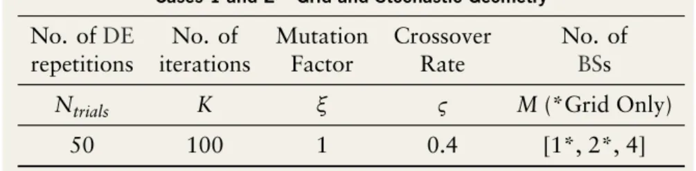
4.3 Simulation Cases . . . 46
4.4 Fitness Functions . . . 47
4.5 Environment Parameters . . . 47
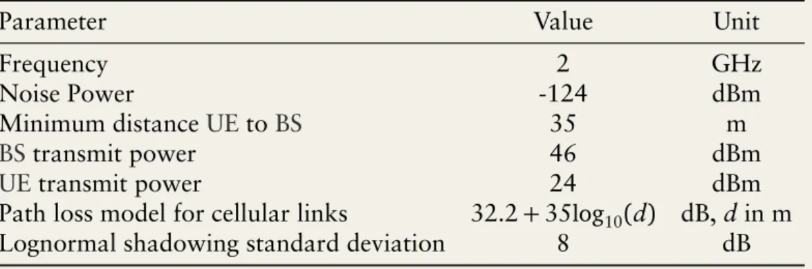
4.5.1 LTE Parameters . . . 48
4.5.2 Trafic Model . . . 49
4.6 Optimization Techniques Parameters. . . 49
4.6.1 PSO Parameters . . . 50
4.6.2 DE Parameters . . . 50
4.7 Network Performance Metrics. . . 51
4.8 Summary of System Model . . . 51
5 Results 52 5.1 Case 1 – Grid layout . . . 52
5.1.1 Fitness Function . . . 52
5.1.2 Performance Results . . . 54
5.1.3 Optimized Points . . . 57
5.1.4 Summary of Optimization in Case 1 . . . 58
5.2 Case 2 – Stochastic Geometry . . . 59
5.2.1 Performance Results . . . 59
5.2.2 Network Performance Metrics . . . 61
5.3 Case 3 – Real Data Based. . . 65
6 Conclusion and Future Work 68
LIST OF FIGURES
1.1 A multi-tier network composed with different kinds of cells . . . 19
2.1 Network index functions . . . 30
3.1 Update of individuals in PSO . . . 34
3.2 Recombination process in DE . . . 38
3.3 DE optimization process lowchart . . . 38
3.4 Update of individuals in DE . . . 38
4.1 Layouts for BS initial deployment regions. . . 42
4.2 Variation of population densityλ according to each neighbourhood . . . . 44
4.3 Trafic demand estimation and BS positions for City 1 . . . 45
4.4 Diagram of UEs deployment . . . 46
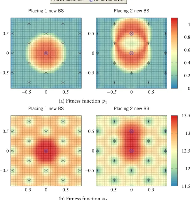
5.1 Fitness functionsφ in Grid layout . . . 53
5.2 Cumulative Distribution Functions (CDFs) of number of iterations until ind best solution in DE – Grid layout . . . 55
5.3 PSO and DE performance for 8, 16 and 32 individuals – Grid layout . . . 56
5.4 PSO performance – Fitness functions φ in Grid layout. . . 57
5.5 DE performance – Fitness functions φ in Grid layout . . . 58
5.6 CDFs of number of iterations until ind best solution in DE when number of new BS = 1 – Stochastic Geometry layout . . . 60
5.7 CDFs of number of iterations until ind best solution in DE when number of new BS = 2 – Stochastic Geometry layout . . . 60
5.8 PSO and DE itness performance for 8 individuals placing 1, 2 and 4 new BSs – Stochastic Geometry . . . 61
5.9 PSO and DE itness performance for 16 individuals placing 1, 2 and 4 new BSs – Stochastic Geometry . . . 62
5.10 PSO and DE itness performance for 32 individuals placing 1, 2 and 4 new BSs – Stochastic Geometry . . . 62
5.11 PSO and DE network performance for placing 4 new BSs with 8 and 16 individuals – Stochastic Geometry . . . 63
5.12 PSO and DE network performance for 32 individuals placing 1, 2 and 4 new BSs – Stochastic Geometry . . . 64
5.13 Fitness φ2∗versus Iteration in Case 3 . . . 66
5.14 Capacity improvementversusIteration in Case 3 . . . 67
LIST OF TABLES
4.1 Large-scale fading model parameters for urban-micro environment. . . 48
4.2 Large-scale fading model parameters for urban-macro environment . . . . 48
4.3 Parameters for LTE throughput (Simulation Cases 1 and 2) . . . 49
4.4 Parameters for PSO optimization – Simulation Cases 1 and 2 . . . 50
4.5 Parameters for PSO optimization – Simulation Case 3 . . . 50
4.6 Parameters for DE optimization – Simulation Cases 1 and 2 . . . 50
5.1 Parameters for Simulation Case 1 – Grid Layout . . . 52
5.2 Fitness results and best points found by PSO in 50 trials . . . 54
5.3 Mean number of iterations until DE ind best solution . . . 54
5.4 Fitness results and best points found by DE in 50 trials . . . 55
5.5 Parameters for Simulation Case 2 – Stochastic Geometry (SG) layout . . . 59
ACRONYMS
1G 1st Generation
2G 2nd Generation
3G 3rd Generation
3GPP 3rd Generation Partnership Project
4G 4th Generation
5G 5th Generation
AWGN Additive white Gaussian noise
BS Base Station
BSP BSPlacement
CDF Cumulative Distribution Function
CoMP Coordinated Multi-Point
dB Decibel
DE Differential Evolution
DL Downlink
EE Energy Eficiency
eNB Evolved Node B
GA Genetic Algorithm
GPS Global Positioning System
HCPP Hardcore Point Process
HetNet Heterogeneous Network
ISD Inter-site Distance
LOS Line of Sight
LTE-A LTE-Advanced
LTE Long Term Evolution
MC-eNB Macro-Cell Evolved Node B (eNB) MIMO Multiple-Input Multiple-Output
MMSE Minimum Mean Square Error
mmW Millimeter Wave
ACRONYMS 14
NP-hard Non-deterministic Polynomial-time hard
PC Personal Computer
PC-eNB Pico-CelleNB
PCP Poisson-cluster Process
PDF Probability Density Function
PL Path Loss
PPP Poisson Point Process
PSO Particle Swarm Optimization
QAM Quadrature Amplitude Modulation
QoS Quality of Service
RATs Radio Access Technologies
SC-eNB Small-CelleNB SG Stochastic Geometry
SINR Signal to Interference-plus-Noise Ratio
SISO Single-Input Single-Output
SNR Signal to Noise Ratio
UE User Equipment
NOMENCLATURE
x Spatial position ofUEs andBSs, page 23
PL Path Loss, page 24
MUE Number ofUEs, page 24
NBS Number ofBSs, page 24
R Distance betweenBSandUE(m), page 24
GTX Gain of transmitter antenna (dB), page 24
GRX Gain of receiver antenna (dB), page 24
pmn Received power (dBm), page 24
W Matrix of received power (dBm), page 24
wm Received power of a singleUEfrom allBSs (dBm), page 24
PTX Transmission Power (dBm), page 24
ψ Received power from servingBS(dBm), page 24
SINR Signal to Interference-plus-Noise Ratio (SINR) sensed by user (dB), page 25
N0 Environment power noise (dBm), page 25
C User capacity, page 25
BW System Bandwidth, page 25
Ctotal Sum of Capacities from all users, page 25
ℓ Throughput limit forBS, page 25
τ Maximum offered capacity for users, page 25
load Trafic demand forBS, page 26
ACRONYMS 16
L Number of newBSs, page 28
S Solution for theBSPproblem, page 28
x Ratio ofBSload and maximum throughput, page 29
N(xn) Fitness function considering network ratiox, page 30
J Jain’s Index, page 31
M Number of individuals forPSOandDE, page 32
xi Positions ofPSOindividuals, page 33 ⃗
vi Velocities ofPSOindividuals, page 33
x∗
i Particle bestPSOindividual, page 33
x∗
g Global bestPSOindividual, page 33
ϕ∗ Random perturbation inPSOupdate, page 34
cgB Acceleration coeficient for global best position inPSO, page 34
cpB Acceleration coeficient for individual best position inPSO, page 34
K Number of iterations, page 35
vi Donor vector inDE, page 37 xi Target vector inDE, page 37
ς Crossover rate, page 37
ui Trial vector inDE, page 37
ξ Mutation factor, page 37
Rearth Earth radius, page 41
λ Density of points – Poisson processes, page 41
φi Latitude, page 41
λi Longitude, page 41
NOMENCLATURE 17
φ Fitness function for optimization, page 47
1. INTRODUCTION
T
hischapter introduces the main motivations of this work in Section1.1followed by a review of the state of the art of theBSPproblem in Section 1.2, where I present the evolution of network planning strategies. I list the objectives, major contributions of this work and thesis organization in Sections1.3 and1.4, respectively. Finally I present my scientiic production during the master course in Section1.5.1.1 Motivation
The continuous development of wireless communications systems, since early gen-erations to advanced technologies, has made possible the growth of such volume of mobile services hard to be imagined half a century ago. Thanks to the development of Electronics and Telecommunications Engineering in the past 40 years, with the exponential growing of electronic hardware computational power and more eficient usage of wired and wire-less channels, it seems there is no boundaries for the worldwide, personal and eficient mobile communications, allowing people to be in contact with each other effortlessly.
However, as new mobile communication services become available, the usage of these services begin to grow rapidly. Recently, the amount of Internet accesses from smartphones and tablets considering only mobile applications overtook Personal Com-puters (PCs) Internet usage in the United States [1]. The increase of smartphone usage is expected to be about 35%per year [2] , but there is a question: are the operators ready to support this growing with current technology?
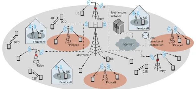
For next wireless networks generations, i.e., 5G, wireless networks are expected to be a mixture of network tiers of different sizes, transmit powers, backhaul connec-tions, several Radio Access Technologies (RATs) that are accessed by an unprecedented number of smart and heterogeneous wireless devices [3]. Thus, the heterogeneity and in-creasing number of network nodes, shown in Figure1.1, will make it dificult to perform infrastructure planning.
CHAPTER 1. INTRODUCTION 19
Picocell Relay
Macrocell
UE
Picocell Picocell
Femtocell UE
Femtocell UE
Femtocell UE UE
D2D Relay D2D
UE D2D
Mobile core network
User broadband connection
Relay D2D
Internet
Figure 1.1: A multi-tier network composed with different kinds of cells
the most important design tasks because it represents capital expenditure for operators, so that ideally it must be done as to improve user’s satisfaction proportionally. There is still room for studying theBSPlacement (BSP) problem because each mobile communications generation proposes different set points of requirements.
1.2 State of the Art
In early wireless network generations, it was established the radio planning had to start from the predictions of coverage to estimate the number of base stations to cover a given area [4], so 1st Generation (1G) and 2nd Generation (2G) planning design were more oriented to coverage, but with the evolution of mobile technologies the rapidly growing usage of broadband made the data rates experienced by the users in the network become increasingly important [5], i. e., the infrastructure expansion planning in 3rd Gen-eration (3G) was more oriented to capacity, leading to high throughput. The paradigm for 4thGeneration (4G) cellular networks was lead towards a high-data rate, low-latency and packet-optimized radio access technology [6], resulting in an improvement of experi-enced data-rates by two and three times on Uplink (UL) and Downlink (DL), respectively compared to the previous generation and the use of lat architecture with radio-related functionalities located in theBS[7]. This results in attainment of multiple services with demanding data-rates, such as high quality video streaming for mobile devices. Finally, besides improvement on data rates, it is expected an alignment for 5th Generation (5G) networks with Energy Eficiency (EE).
CHAPTER 1. INTRODUCTION 20
attain success in the market, operators normally use strategic and operative software tools for designing, planning and optimizing wireless networks, which are money-savers for their business. Nevertheless, while operators keep providing wireless access services, the technologies change demands repetition of network planning tasks based on new requirements. Thus, it is very common to observe two or three different technologies supported by an operator at the same time in order to satisfy many users’ requirements simultaneously. Finally, the plan of deployingLTE 4Gnetworks to satisfy the increasing of trafic demands translates into a continuous need forLTEcell sites planning [9].
1.2.1 Network Planning Issues
The BSP optimization task depends on a set of variables, such as trafic density, channel condition, interference scenario, number ofBSs, etc. [10] deines the cell planning problem as searching for a subset of base stations’ positions{BSo} ⊆ {BS∗}that satisies desired criteria, where{BS∗}corresponds to all possible conigurations forBSs. Because of the relation and combination between these variables, BSP is an Non-deterministic Polynomial-time hard (NP-hard) problem [11] for which it is not possible to ind a poly-nomial time algorithm in the theory of computational complexity. Instead of perform-ing exhaustive combination of all possibilities as solution of this problem, many works suggested strategies using specially evolutionary and heuristic algorithms. A general op-timization algorithm is implemented to optimizeBSplacement in a very realistic scenario containing a large set of variables. However, this large number of attributes makes al-gorithms’ runtime very long. On the other hand, limiting the set of variables produces coarse results. Furthermore, the optimization problem can be formulated with various objectives, for example: capacity enhancement, network lifetime maximization, power and node number minimization [12].
1.2.2 Heuristics forBSPoptimization
Some applicable heuristic methods for theBSPproblem are described below: • Particle Swarm Optimization (PSO):It was introduced by [13] in 1995 as an optimization
CHAPTER 1. INTRODUCTION 21
various UE distribution. These works considered network planning for the irst placement ofBSs. PSOhas also been tested on wireless network optimization, such as sensor’s coverage [17].
• Differential Evolution (DE): It was presented to scientiic community by the year of 1995 in the First International Competition on Evolutionary Optimization by Price and Storn [18]. The strength of the algorithm lies in its simplicity, speed and robustness [19]. Also, DEwas veriied in wireless sensors network optimization in [20] with the goal of inding the best operational mode for each sensor in order to minimize energy consumption.
1.3 Objectives and Major Contributions
The objectives of this work are described as follows:
• Present theBSPtask as an optimization problem;
• AdaptPSO and DE to the BSP problem for the placement of a single or multiple bases and evaluate their performance by measuring their itness;
• Apply these heuristic methods in a real-based scenario consisting on real informa-tion ofBSs’ position and trafic estimates derived from population data;
As main contribution, this work validates the use of PSOandDEas suitable tech-niques forBSPoptimization. The speciic objectives are:
• Deinition of itness functions for optimization process based on network aspects in Chapter2;
• Modelling of many wireless network scenarios in Chapter4;
• ComparePSOandDEperformance for those layouts in Chapter5.
1.4 Thesis Organization
CHAPTER 1. INTRODUCTION 22
shown in Chapter5for all scenarios described previously in Chapter4. The summary of simulation results and further expectations of this work is exhibited in Chapter6.
1.5 Scientiic Production
The following work was submitted and accepted for a conference during the Master period.
2. BASE STATION PLACEMENT MODELLING
E
evaluatingtheBSP optimization problem requires mathematical modelling in or-der to verify the practicability of obtaining an exact solution using a close expression or either applying an optimization technique. This chapter exhibits mathematical devel-opment for modelling this problem regarding a region composed of sets ofBSs andUEs with two dimensional positions.2.1 Fundamentals
Wireless propagation radio channels confront several issues. In fact, the wireless signals suffer severe attenuation in links betweenBSs and UEs caused by dissipation of the power radiated by the transmitter as well as effects of the propagation channel. The modelling of attenuation on received signal strength in the receptor can be assumed as
physicalorstatistic: the second one takes empirical approaches, measuring propagation characteristics in a variety of domains and developing these models for a class of particular environments [21]. From these statistical representations, attenuation depends on many parameters which can be split in two parts: thepath lossandshadowing, described below:
• Path Loss (PL)is the ratio of transmitted pT and receivedpR power, which can be given in linear scale or in Decibel (dB) scale (2.1):
PL= pT
pR → PLdB=10log10PLdB. (2.1)
Because most mobile communication systems operate in complex propagation en-vironments that cannot be accurately modelled by free-space path loss or ray trac-ing, many path loss models have been developed over the years [22] to predicting channel effects in many environments. These theoretical and measurement-based propagation models indicate that average received signal strength decreases with the distance R between transmitter and receiver [23]. The value of R depends on the absolute distance between spatial positions from sets of MUEs and NBSs, where eachUEmandBSncontain spatial positions represented byUEm(x)andBSn(x), re-spectively, such thatx= [x1x2]in a two-dimensional plane. The distance between these nodes is given byRmn, which denotes their absolute distance as shown in (2.2):
CHAPTER 2. BASE STATION PLACEMENT MODELLING 24
Given an empirical pathloss model and the distance Rmn between each UEm and
BSn, thePLmncan be obtained by any general expression (2.3):
PLmn=pathloss(Rmn). (2.3)
• Shadowing(χ) is caused by obstacles between the transmitter and receiver that at-tenuate signal power through absorption, relection, scattering, and diffraction [22]. This effect was also veriied empirically and is often modelled as a log-normal ran-dom variable with mean µχ and standard deviationσχ, deined for each empirical scenario.
Eventually, experimental models depend on deinitions of the environment characteristics, such asBSantenna heights, average building height, distance between buildings, etc. Such information will be detailed in Chapter4.
Considering the downlink scenario, theBSs andUEs are the transmitter and receiver nodes, respectively, from which eachBSnhas transmission powerPTXn , orPBSn . Also, other attributes are deined for downlink case in order to model the links betweenBSs andUEs, such as antenna gainsfor transmitter GTX
n , or GBSn , and receiver GRXm , or GUEm , given in dB, which depend on the radiation pattern of these antennas. With possession of these attributes, the received powerpmnat theUEmfromBSn is estimated by:
pmn=PBSm +GBSm +GUEn −PLmn+χmn. (2.4)
From received power values, pmn, the matrix W presents signal strengths from all links betweenUEs andBSs (2.5):
W=
p11 p12 · · · p1N p21 p22 · · · p2N ... ... ... ...
pM1 pM2 . . . pMN
=
w1
w2 ... wM
, (2.5)
where row vectorswm= [pm1pm2 · · · pmN]collect the received powers for UEm from all
BSs.
The highest value in each vectorwm is the maximum received power forUEm. As-suming the maximum received signal strength corresponding to power received from the servingBS, the other values inwmare interpreted as interfering signals from all remaining bases. Considering the following statement:
CHAPTER 2. BASE STATION PLACEMENT MODELLING 25
ψm=max(wm), (2.6)
if each BS uses all network spectrum resources and all links between BSs and UEs are assumed as active in the network, theSINR is obtained as follows (2.7), given ψm and
wm converted from dB to linear scale:
SINRm= ψm
N
∑
n=1pmn−
ψm+N0
, (2.7)
whereN0denotes the Additive white Gaussian noise (AWGN) power noise. The expres-sion ∑N
n=1
pmn−ψmis the sum of the powers received from allBSs minus the power incoming from the servingBS, thus resulting in the sum of the interference contributions, since the network model assumes a fully loaded system, in which all links are active. Finally, from Shannon equation [24], the capacityCfor this coniguration is denoted by:
Cm=BW·log2(1+SINRm) bps, (2.8)
whereBWdenotes system bandwidth. A general expression assumesBW=1 and returns capacity in bits per second per Hertz (bps/Hz).
2.1.1 System Capacity
The capacity shown previously (2.8) is evaluated for a single user under the prop-agation characteristics described in Section2.1. Supposing the network has fully loaded links betweenUEs andBSs, which are presumed to potentially serve all these users in its full demand, the theoretical total capacity that could be sensed by users is interpreted as the sum of single capacities forUEs (2.9):
Ctotal= M
∑
m=1
Cm. (2.9)
Although the amount of capacity sensed by users considers only theirSINRs (2.8), in a multicellular scenario theBSs have a maximum trafic which can be offered to connected UEs. It means that the provided capacity for users is limited by the sum of the maximum allowed trafic of allBSs. Assuming eachBShas a throughput limit ofℓn, the maximum capacityτoffered for users becomes:
τ=
N
∑
n=1
CHAPTER 2. BASE STATION PLACEMENT MODELLING 26
Thus, the total offered capacityτmight be higher or lower than the sum of sensed capac-itiesCtotaldepending on the network planning. The choice of trafic model impacts on the network evaluation by means ofBSs overload. Adopting a full buffer trafic characterized by a ixed number of users in the cell and the buffers of the users’ data lows always hav-ing unlimited amount of data to transmit/receive [25] require full dimensioning of users’ demand.
2.1.2 Base Station Load
The measurement ofBSs’ load depends on the amount of trafic demanded by each BS, associating users with bases that provide the strongest power for them. From (2.6), the maximum value of wm is equivalent to its received power, therefore, the position where the highest value is found corresponds to the index ofBSthat services theUEm.
Considering the subset ofM∗UEs as{UE
1,UE2,· · ·,UEM∗}nthat are connected only toBSn and assuming their capacities as{C1,C2,· · ·,CM∗}n, the expected load for a single BSis:
loadn= M∗ ∑
m=1
Cm. (2.11)
The measurements on theBSload capture a more speciic characteristic of network in terms of BSs’ overload. For example, the offered capacity, τ, can be equal to users’ demand,Ctotal, but existing anyBS, BS
n, where the loadloadn is higher than its offered throughput,ℓn. From the evaluation of BSs loads, a measurement of overload of bases can be asserted and regions where users are affected by high trafic load can be mapped.
2.2 Optimization Problem Formulation
The optimization problem consists of inding a solution with either maximum or minimum measurement [26] for a itness or objective function. A mathematical optimiza-tion problem has the following form [27]:
minimize f0(x)
subject to fi(x)≤bi, i=1,· · ·,m.
(2.12)
The vectorx corresponds to theoptimization variable and the function f0 : IRN → IRis theobjective function, the functionsfi: IRN →IRare constraint functionsandb1,· · ·,bm correspond to limits for constraints.
CHAPTER 2. BASE STATION PLACEMENT MODELLING 27
Polynomial-time hard (NP-hard), which cannot be solved by algorithms in polynomial time. Furthermore, if objective or constraint functions are not linear and not known to be convex, the general non-linear programming problem shown in (2.12) requires alternative optimization algorithms, which is the case of capacity-based objective functions.
2.2.1 Inserting NewBSs
The problem formulation starts by modelling the positioning of a new BS in the environment. Rewriting the received power matrix (2.5) when inserting one newBSas:
W=
p11 p12 · · · p1N p1N+1
p21 p22 · · · p2N p2N+1 ... ... ... ... ...
pM1 pM2 . . . pMN pMN+1 =
w1 p1N+1
w2 p2N+1 ... ... wM pMN+1
= w∗ 1 w∗ 2 ... w∗ M , (2.13)
where the column N+1 contains powers obtained when setting a single new BS. The expressions forSINRand capacity shown in (2.7) and (2.8) differ only in theψvalue due to the changing on the interference originated from inserting new bases. The maximum received powerψmfrom (2.6) becomes:
ψ∗m=max pm1,pm2,· · ·,pmN,pm,N+1
,
ψ∗m=max w∗ m
. (2.14)
Although the placement of a new baseN+1 increases total offered throughput by τ+ℓN+1, the users’ sensed sum of capacities would increase or diminish due to interference effects.
When using capacity-based functions as itness, the optimization problem isNP-hard, since the individual users’ capacities (2.11) depends on theSINRs, which is a non-linear function ofBS’ positionsx. The placement of a single newBScan determine an approxi-mate optimal positionxa prioriby using one of the following methods:
• Exhaustive Search by disposing random points in the map and test each one on the itness function, for which precision varies with the number of trials for inding minimum or maximum.
• Grid Method by creating a grid set of points and testing all of them. The precision depends on the length of data set, i.e., on the grid spatial resolution.
CHAPTER 2. BASE STATION PLACEMENT MODELLING 28
size of the search space and the desirable precision, the solution can be obtained with a good accuracy with relatively low number of tests, e.g., thousands of points.
Now assuming the placement of Lnew bases, (2.13) can be rewritten considering multipleBSs as shown below:
W=
p11 p12 · · · p1N p1N+1 · · · p1N+L
p21 p22 · · · p2N p2N+1 · · · p2N+L ... ... ... ... ... ... ...
pM,1 pM2 . . . pMN pMN+1 · · · pMN+L =
w1 p1N+1 · · · p1N+L
w2 p2N+1 · · · p2N+L ... ... ... ... wM pMN+1 · · · pMN+L
= w∗ 1 w∗ 2 ... w∗ M . (2.15)
The placement ofLnewBSs will increase the offered throughput toτ+∑Ll=1ℓN+l, corresponding to a potentially substantial improvement on the network throughput. On the other hand, the amount of interference ∑N+L
n=1 pnm−ψm will be greater, causing the users’ sensed capacity to be lower, thus decreasing the Quality of Service (QoS) of net-work.
In the case of placingLnew bases, the search for nearly optimal solutions increases exponentially withL, because it is necessary to test every combination ofLpossible new solutions.
2.2.2 Runtime Analysis
Consider both approximate methods for searching optimal points described in2.2.1 and ignoring the complexity of evaluating the itness function, assume that inding the optimal position for inserting one single base requires testingKcandidate positions. Now, assumingS(1)as the solution for placing this one new base, consider as true the following statement:
S(1)⊇ {x1}. (2.16)
Then, expanding this solution to placeLbases leads to:
S(2)⊇ {x1,x2}
S(3)⊇ {x1,x2,x3} ...
S(L)⊇ {x1,x2,· · ·,xL}.
CHAPTER 2. BASE STATION PLACEMENT MODELLING 29
Since the irst solutionS(1)is obtained after testingKpoints, the search of solutionS(L) requires testing KL sets of points to ind the solution[x
1 x2 · · · xL]. Depending on the calculation time for measuring itness, this growing of the number of required operations makes it dificult to use the exhaustive search technique. Moreover, due to the fact that variations in the set of positions forBSs affect theSINRvalues, the optimal points might be different for any solution.
2.3 Fitness Functions
Fitness functionsare used to compare different solution sets or make optimization processes converge to a global value. The itness functions are composed by some objec-tive criteria that evaluate the performance of: 1) only newBSs or 2) the entire network. The combination of measurements on demanded capacity of usersCtotaland overload of basesloadnresults into the deinition of our itness functions: theNetwork Index, which aims to maximize performance ofBSs without overloading them, and thecapacity max-imization with load balancing, whose objective is balancing BSs load and maximizing users’ sensed capacity simultaneously. These itness functions are described in following subsections.
2.3.1 Function 1: Network Index
Assuming each BS has a maximum throughput ℓn, the amount of resources that can be shared for all connectedUEwill be limited even if the sum of capacities of users is greater thanBS maximum throughput. The metric called network ratio xn deined here establishes a factor to measure the overload ofBSand it equals the ratio between theBS load described in (2.11) and its throughput limitℓn(2.18):
xn= ∑M∗
m=1Cm
ℓn ,
xn= loadn
ℓn · (2.18)
Based on the domain of variablexn∈[0,∞), let us make the following assessments:
• Case 1: Whenxn<1, the sum of throughputs of users is lower than theBS’s through-put maximum, thus, the requirements of users will be fully served, but the base has not been demanded on its limit yet;
CHAPTER 2. BASE STATION PLACEMENT MODELLING 30
demands;
• Case 3: In the case ofxn=1, theBShas assigned all its capacity for all users, fulilling their requirements.
For a wireless network, the aim is the optimization of positions for nodes in order to make each BS close tocase 3 operation because the amount of available resources is equal to users’ demands. Thus, the objective function must map xn so resulting on its highest value whencase 3is achieved. DeiningN(xn)as objective function, it is designed to have imageN(x)∈[0,1], with maximum atx=1 and minimum at 0 and∞in order to focus optimization towards case 3. Moreover, the mapping of these cases to itness values results in the continuous functionη1= N(xn) suitable to represent the effects of overload as:
N(xn) =xnα·e(1−xnα) , α∈IR : α≥2. (2.19)
Figure2.1exhibits the network index functions (2.19) emphasizing that the variation ofα parameters affects the sensitiveness for very low or large values ofx. The itness function has no unity for its values.
P493p Pe
obj
0 0.5 1 1.5 2 2.5 3
0 0.2
0.4
0.6
0.8
1
Network Ratiox
Fitness
η1(x), α=2 η1(x), α=2.5
η1(x), α=3 η1(x), α=4
Figure 2.1: Network index functions
2.3.2 Function 2: Capacity Maximization with Load Balancing
The capacity maximization with load balancing metric targets the increase of the mean throughput of all users, based on total capacity, Ctotal, (2.9), while balancing the BSs load,loadn, (2.11).
CHAPTER 2. BASE STATION PLACEMENT MODELLING 31
Index JforBSs loads (2.20) is given as:
J=
∑N
n=1loadn
2
N·∑Nn=1loadn2
. (2.20)
The variableloadn∈[0,∞]results inJ∈[1/N,1]. Moreover, the valueJ=1 means that allBSs have the same load demand.
Now supposing the set of MUEs which has mean throughput equals to:
C= C
total
M , (2.21)
thus, combining theJvalue with the users total throughput mean demandC(2.22):
η2=J·C. (2.22)
2.4 Summary of Base Station Placement Modelling
3. SPATIAL OPTIMIZATION TECHNIQUES
M
anyoptimization problems focus on maximization or minimization of itness func-tions, but the optimization using classical approaches may be onerous if the search space of the utility function is hard to be modelled mathematically. As discussed in Sec-tion2.2.1, for the BSP problem, each new point inserted in the search space affects the overall performance parameters for all network nodes. Even for inding a nearly opti-mal solution, thisNP-hardproblem requires an exhaustive combinatorial search, which makes the simulation time grow very quickly depending of the number ofBS positions for combination.Under these conditions, some heuristic-based methods for inding nearly-optimal solutions might be considered, since they present good results without a very high com-putational cost.
This chapter presents two methods of inding good near optimal solutions: Par-ticle Swarm Optimization (PSO) and the Differential Evolution (DE), both inspired by biological and sociological motivations and able to take care of optimality on rough, discontinuous and multi-modal surfaces [19].
3.1 Particle Swarm Optimization
3.1.1 Fundamentals
The Particle Swarm Optimization (PSO) is a population-based stochastic algorithm for optimization inspired by social-psychological principles [29]. PSOdiffers from other evolutionary algorithms because it uses all population members from the beginning of a trial until its end. The principle ofPSOis based on the idea that these population individ-uals move within the solution space inluencing each other with stochastic changes, while previous successful solutions act as attractors [30]. Thus, the interactions of individuals with each other result in incremental improvement of the quality of problem solutions over time.
CHAPTER 3. SPATIAL OPTIMIZATION TECHNIQUES 33
inluenceandpersistence; and considering some random perturbation.
3.1.2 Mathematical Representation
When representing problem in a IR2 space, each particle Pi in PSO contains two vectors with same dimension as the search space. The position of particle is represented by a vectorxi (3.1a) while its velocity is represented by⃗vi (3.1b) ; both attributes relates to the same iterationk. Given current position and velocity of a particle, PSOperforms the movement of individuals by updating position withxi[k+1]in the next iterationk+1 obtained by adding currentxi[k]and⃗vi[k]in iterationk(3.2):
Pi
x
i= [x1x2]i, (3.1a)
⃗
vi= [v1v2]i, (3.1b)
xi[k+1] =xi[k] +⃗vi[k]. (3.2)
Assuming a random deployment of individuals and a random selection of their velocities as initial conditions, the update of positions and velocities depends on the be-haviour of particles regarding the itness function within the search space. Two major factors affect the optimization process:
• Persistence, which considers the best position reached by a single individualPi, the
best particlerepresented byx∗
i. The persistence on the particlePi is:
persistence= x∗i −xi[k],
thus, this parameter measures how far is the position ofPito the best position found byPSO;
• Social Inluence, which relates to the best position ever found by the entire set of particles, called also global best and represented as x∗
g. The social inluence on particlePi is represented by:
social inluence=x∗g−xi[k],
so this attribute calculates distance of the position of Pi and the best position ever found by the group of particles.
CHAPTER 3. SPATIAL OPTIMIZATION TECHNIQUES 34
Thus, one has
⃗
vi[k+1] =⃗vi[k] +ϕi∗· x∗i −xi[k]
+ϕ∗g·x∗g−xi[k]. (3.3)
Moreover, (3.3) can be verbally read as:
NEW VELOCITY = CURRENT VELOCITY + PERSISTENCE + SOCIAL INFLUENCE. (3.4)
Therefore, the update of positions assumes new velocities obtained in every optimization iteration.
Theϕ∗
i andϕg∗parameters determine the strength of random perturbations towards global and individual best positions P∗ind
i e P∗global [31], also called acceleration
coefi-cients. Each of these perturbations can be rewritten as a product of the formϕ∗=c·ϕ, wherecis a known scalar andϕ is a uniform random variable between 0 and 1. Each in-luence attribute is scaled with constantscgB andcpB, respectively. The update of velocity in (3.5) is represented by:
⃗
vi[k+1] =vi[k] +cpB·ϕi· x∗i −xi[k]+cgB·ϕg·x∗g−xi[k]. (3.5)
The effect of individuals update in PSO for a 2-dimensional search space is shown in Figure3.1.
Global Best Particle Next Iteration
Particle Best
Current Particle
x ∗ −g
x[ik ]
⃗
vi[k
]
x∗
i −xi[k
]
⃗ vi[k
+1]
ϕ
∗ ·g x
∗ −g x[ik
]
ϕ∗i · x ∗
i −xi[k
]
xi[k]
x∗
g
x∗
i
xi[k+1]
CHAPTER 3. SPATIAL OPTIMIZATION TECHNIQUES 35
3.1.3 Improvements in PSO topology
Some studies proposed improvements in PSO by including an inertia weight for velocities and updating both social inluence and persistence parameters, as shown below:
1. Inertia coeficient: As proposed in [32], the inclusion of a decreasing coeficient for velocities’ update is effective for reducing the inertia of the particles. This character-istic stabilizes the position of individuals in late iterations. Assuming Kiterations, and given initial w0 and inal wK values for inertia, w[k] for each iteration k are equal to:
w[k] =w0+ k
K·(wK−w0). (3.6)
That variation in inertia coeficient affects exploration, when individuals are lead to search towards new unexplored regions, and exploitation, when they take ad-vantage of positions where good itness values were found previously.
2. Variation in Social Inluence and Persistence: The work of [33] assumes also a temporal variation for social and individual attributes,cgBandcpB. This concept emphasizes local or global search in different periods of optimization, similar to the idea of variation in acceleration discussed previously. Given initial and inal values forcgB andcpB as{c0,cK}, the variation of both coeficients is performed by:
c[k] =c0+ k
K·(cK−c0). (3.7)
Regarding these two improvements, a general update for velocities inPSObecomes:
⃗
vi[k+1] =w[k]·⃗vi[k] +cpB[k]·ϕi· x∗i −xi[k]
+cgB[k]·ϕg·x∗g−xi[k]. (3.8)
3.1.4 Simulation Chain
CHAPTER 3. SPATIAL OPTIMIZATION TECHNIQUES 36
Algorithm 1PSOalgorithm
1: Set up initiallyMparticlesPi,i=1, . . . ,M 2: Deinew0,wK,cpB andcgB
3: for allParticlesPi do 4: Setxi andvi 5: end for
6: SetP∗ind←P
1 andP∗global←P1 7: forKiterationsdo
8: Compute accelerationwk←w0+ (k/K)·(wK−w0)(3.6) 9: for allParticlesPi do
10: compute itnessηi,η∗indandη∗global forP
i,P∗indandP∗global 11: ifηi ≷η∗ind then
12: P∗ind←P i 13: end if
14: ifηi ≷η∗global then
15: P∗global←P
i 16: end if
17: persistence←ϕ·(Pi−P∗ind) 18: social inluence←ϕ·(Pi−P∗global)
19: ⃗vi←wk·⃗vi+cpB·persistence+cgB·social inluence(3.8) 20: xi←xi+⃗vi (3.2)
21: end for 22: end for
3.2 Differential Evolution Optimization
3.2.1 Fundamentals
Differential Evolution (DE) is a stochastic parallel search method for maximization or minimization of itness functions [34]. DE was originally designed to handle opti-mization of real-valued functions based specially on the use of a differential operator to create new individuals for following generations, which is an advantage compared to the classical Genetic Algorithm (GA), designed for discrete search spaces.
This technique performs a parallel search in aN-dimensional region usingMsingle entities, with the same dimension of the search space, as population for each generationk, attempting to replace all points in search spaceSby new positions at each generation [35]. A general formulation for optimization of theDE-based is to indx∗ given the objective functionf:X⊆IRN→IR, i. e.:
x∗∈X|f(x∗)≷f(x) ∀x∈X, (3.9)
CHAPTER 3. SPATIAL OPTIMIZATION TECHNIQUES 37
3.2.2 Mathematical Representation
Similar to other evolutionary algorithms, DE starts the searching process with M
individuals whose positions are represented byxi. Thus, for aIR2search space:
xi= [x1x2]i. (3.10)
AssumingKgenerations for the optimization process, each trial performsMutation, Re-combinationandSelection, as described below:
• Mutation expands the search space by giving ways for generating new individuals. For all x individuals in each iteration k, the process chooses four of them xi, xr1, xr2 andxr3, withi̸=r1̸=r2̸=r3. The individualxi is calledtarget vector and the individualxr1is added to the weighted difference betweenxr2andxr3given by:
vi=xr1+ξ·(xr2−xr3), (3.11)
whereξ is themutation factorandvi is thedonor vector for thek-th iteration.
• Recombination incorporates solutions that resulted in successful itness performance previously. This process generates thetrial vectorui from a combination of target, xi, and donor vectors, vi. Each vector position is denoted by j. Giving ς as the probability that elements of donor vector replace elements of the target vector – the
crossover rate– and givingφ[j]as a uniform random variable, we have:
ui[j] =
vi[j],
xi[j],
φ[j]≤ςORj=ι,
φ[j]> ςANDj̸=ι, (3.12)
whereιis a discrete random variable∈[1,2,· · ·,N]which avoiduito become equal toxi– at least one value of the donor vectorviwill be propagated to its offspringui. Figure3.2shows how recombination process works: the trial vector will be illed by elements of either the target or donor vectors, if conditions are satisied (3.12). • Selectioncompares the itness values provided by thei-th trial and the target vectors.
If the trial vector results in better itness, the individual that provides the target vector is replaced by the trial vector as shown:
xi=
ui, ifη(ui)≤η(xi),
xi, otherwise.
(3.13)
CHAPTER 3. SPATIAL OPTIMIZATION TECHNIQUES 38 · · · · · · · · · · · · · · · · · · · · · · · · · · · · · · · · · · · · · · · · · · · · · · · · · · · · · ·
x[1] u[1] v[1]
x[2] u[2] v[2]
x[3] u[3] v[3]
j=ι
· · · u[j] v[j]
φj≤ς
φj> ς
x[j] u[j] v[j]
x[N] u[N] v[N]
Figure 3.2: Recombination process inDE
optimization criterion is reached or until at mostKgenerations are simulated, as shown in Figure3.3. Assuming a 2-dimensional search space, the update of individuals by these three processes is graphically shown in Figure3.4.
Initialization Mutation Recombination Selection
until bestηorKgenerations
Figure 3.3: DEoptimization process lowchart
ui
ξ·∆
φ
2
≤
ς
φ1≤ς
φ1,2
≤ς
∆=xr2
−xr3
xr1
v(v1,v2) i
x(x1,x2) i
(x1,v2) (v1,x2)
xr2
xr3
Figure 3.4: Update of individuals inDE
CHAPTER 3. SPATIAL OPTIMIZATION TECHNIQUES 39
3.2.3 Simulation Chain
A generic simulation chain forDEis shown in Algorithm2by providing the muta-tion factor,ξ, and crossover rate,ς.
Algorithm 2DEalgorithm
1: Deineitness targetη∗, mutation factorξ, crossover rateς 2: Set up initialtarget vectorsx
3: for allIndividualsxi do
4: Set positions and get their itnessηi 5: end for
6: Get best itnessηbestof allηi 7: whileηbest≷η∗ do
8: Choose random integersi̸=r1̸=r2̸=r3 9: donor vector
10: vi←xr1+ξ·(xr2−xr3)(3.11) 11: for allPositionsjdo
12: Compute random integerι and random scalarφ 13: Get thetrial vector
14: ifφ≤ςorj=ι then 15: ui[j]←vi[j](3.12) 16: end if
17: ifφ > ςandj̸=ι then 18: ui[j]←xi[j](3.12) 19: end if
20: end for
21: Compute itnessη(ui)andη(xi) 22: ifη(ui)≷η(xi)then
23: xi←ui 24: ηbest←η(ui) 25: end if
26: end while
3.3 Summary of Optimization Techniques
4. SYSTEM MODEL
C
hoosing a proper system model is relevant to perform a fair comparison of op-timization techniques and to simulate how these methods could work using real environment data. There are some techniques to generate a real-based region, which placement ofUEs andBSs not only looks like actual deployment from operators, but also presents similar properties, such as coverage probability. This chapter discusses the gen-eration of environments with differentBSplacement layouts and trafic characteristics.4.1 Multi-cell Scenario
The multi-cell scenario is composed by sets of BSs and UEs distributed over the coverage area and can be generated by many ways, given strategies for placingBSs and modellingUEtrafic. This section discusses three methodologies for deployingBSs: grid layout,stochastic geometryandbased on real data.
4.1.1 Grid Layout
The grid layout is widely used to represent a cellular network, which is composed byBSs distributed in a hexagonal lattice with ixed distance from each other, as shown in Figure 4.1a. The recommendation in [36] adopts a distance equals 500m between BSs (Inter-site Distance (ISD)) and urban-microcell fading environment for path loss and shadowing.
4.1.2 Stochastic Geometry
Stochastic Geometry (SG)can represent the randomness of an actual wireless work allowing to study the average behaviour over many spatial realizations of a net-work whose nodes are placed according to some probability distributions [37]. This network randomness is particularly veriied when working with Heterogeneous Net-works (HetNets). In this scenario, due to the increasing number of nodes, network ele-ments are placed to satisfy ad-hoc requireele-ments.
CHAPTER 4. SYSTEM MODEL 41
BSs because it requires a minimum distanceRfor deploying nearby bases. Indeed, theBS locations appear to form a more regular point pattern than thePPPbecause of repulsion between points [39].
APPPis composed by a setΠof points from which any subsetB⊂Πis composed by Poisson random variables, as follows:
Π={xi,i=1,2,3,· · · } ⊂Rd if, and only if B⊂Πis a Poisson variable, (4.1)
whereRdis thed-dimensional search space.
An HCPP is a repulsive point process where no two points of the process coexist with a separating distance not smaller than a predeined hard core parameterR:
Π={xi,i=1,2,3,· · · } ⊂Rd if, and only if xi−xj
≥R;∀xi,xj∈Π. (4.2)
The deinition of regions withPPPandHCPPpoints require deinition of densityλ forUEs andBSs, usually given in number of points per area unity. Figure4.1bshows the BSs deployment deploying according to aHCPPprocess withR=70m.
4.1.3 Based on Real Data
The real scenario is based on real information ofBSpositions found in some databases such as Brazilian Telecommunications Regulatory Agency (ANATEL) database [40], which gives data from operators in Global Positioning System (GPS) coordinates. Figure 4.1c shows an example ofBSs existing in a Brazilian city.
The evaluation of fading properties requires conversion of distance dependent pa-rameters originally given inGPScoordinates to meters in order to evaluate the distances between points, such as Haversine (great circle) method [41]. Given two points with latitudeφ1,φ2and longitudeλ1,λ2, let∆φ=φ2−φ1 and∆λ=λ2−λ1:
a=sin2
∆φ 2
+cos(φ1)·cos(φ2)·sin2
∆λ 2
,
c=2·asin pa.
Thus, the distance between these two pointsdis given by:
d=Rearth·c, (4.3)
CHAPTER 4. SYSTEM MODEL 42
All scenarios described in subsections4.1.1,4.1.2and4.1.3are shown in Figure4.1, which Grid andSG BSlayouts are described in meters while actual data is represented in GPScoordinates.
−4 −2 0 2 4
−4 −2 0 2 4
(a) Grid layout
−4 −2 0 2 4
−4 −2 0 2 4
(b) Stochastic Geometry: HCPP
−38.65 −38.6 −38.55 −38.5 −38.45 −38.4 −3.85
−3.8 −3.75 −3.7
Latitude
Longitude
BSpoints
(c) Actual Data – City 01
Figure 4.1: Layouts forBSinitial deployment regions
4.2 UE Trafic Positioning and Representation
CHAPTER 4. SYSTEM MODEL 43
heterogeneity of trafic demand in speciic locations of network. In other words, theUEs deployment represents the trafic inside the region of interest. In order to perform this modelling, for the following methods supposing a set ofmUEs with positionsUEm(x),x is the spatial location ofUEand the trafic associated toUEm will be denoted byγm.
For a set of N BSs, assuming the throughput demanded by each BS, n, as Cm,n, and supposing M∗ users connected to that base, the total required throughput can be interpreted as:
Cm,n= M∗ ∑
m=1
Cm. (4.4)
Thus, for user required throughputγm:
Cm,n= M∗ ∑
m=1
γm. (4.5)
4.2.1 Randomly Heterogeneous UEs Deployment
In this technique, all user points are assumed as demanding trafic of the same kind. Thus, high trafic regions can be interpreted as those where a larger amount ofUEpoints can be found. Using this methodology, the evaluation of outage or satisfaction analysis is done by assessing singleUEs performance.
The placement of users non-uniformly distributed is deined by setting up regions whose probability ofUEbe inserted inside differs from each other. The set ofUEm(x)has a probability to be inserted depending onx position.
Since the users’ required throughputs are equal to all points, i.e.,γm=γ∗, (4.5) can be rewritten as:
Cm,n=
M∗ ∑
m=1 γ∗,
Cm,n=M∗·γ∗, (4.6)
which is basically the number of connected UEs scaled to the throughput γ∗. The gen-eration of this kind of environment assumes multiple subregions with varying density of users. Assuming the global environment as R, a region Rk contains particular aspects in terms of trafic demand or user density such that Rk⊂R. The regionRk contains nk
users, so the density of usersλkcan me denoted by:
λk= area(Rk)
nk