Network effects, conformism and misbehavior in Brazilian classrooms

(1)

UNIVERSIDADE FEDERAL DO CEAR ´A

FACULDADE DE ECONOMIA, ADMINISTRAÇ ÃO, ATU ÁRIA E

CONTABILIDADE

PROGRAMA DE P ÓS-GRADUAÇ ÃO EM ECONOMIA

MESTRADO ACADˆEMICO

LUAN FALC ˜AO DANIEL SANTOS

NETWORK EFFECTS, CONFORMISM AND MISBEHAVIOR IN BRAZILIAN

CLASSROOMS

(2)

(3)

LUAN FALC˜AO DANIEL SANTOS

NETWORK EFFECTS, CONFORMISM AND MISBEHAVIOR IN BRAZILIAN CLASSROOMS

Disserta¸cão apresentada ao Programa de Pós-Gradua¸cão em Economia da Universi-dade Federal do Ceará como requisito par-cial para a obten¸cão do T´ıtulo de Mestre em Economia.

Orientador: Prof. Dr. José Raimundo de Araújo Carvalho Júnior

FORTALEZA

(4)

Dados Internacionais de Catalogação na Publicação Universidade Federal do Ceará

Biblioteca Universitária

Gerada automaticamente pelo módulo Catalog, mediante os dados fornecidos pelo(a) autor(a)

S236n Santos, Luan Falcão Daniel.

Network Effects, Conformism and Misbehavior in Brazilian Classrooms / Luan Falcão Daniel Santos. – 2016.

79 f. : il. color.

Dissertação (mestrado) – Universidade Federal do Ceará, Faculdade de Economia, Administração, Atuária e Contabilidade, Programa de Pós-Graduação em Economia, Fortaleza, 2016.

Orientação: Prof. Dr. José Raimundo de Araújo Carvalho Júnior.

1. Peer Effects. 2. Conformism. 3. Networks. 4. Local-average Model. I. Título.

(5)

LUAN FALC˜AO DANIEL SANTOS

NETWORK EFFECTS, CONFORMISM AND MISBEHAVIOR IN BRAZILIAN CLASSROOMS

Disserta¸cão apresentada ao Programa de Pós-Gradua¸cão em Economia da Universi-dade Federal do Ceará como requisito par-cial para a obten¸cão do T´ıtulo de Mestre em Economia.

Aprovada em

BANCA EXAMINADORA

Prof. Dr. José Raimundo de Araújo Carvalho Júnior(Orientador)

Universidade Federal do Cear´a

Prof. Dr. Diego de Maria Andr´e Universidade Federal do Rio Grande do

Norte

Prof. Dr. Victor Hugo de Oliveira Silva

(6)

(7)

(8)

(9)

Resumo

Para entender de que forma as networks afetam o comportamento dos

in-div´ıduos, em espec´ıfico o comportamento de estudantes no ´ultimo ano do ensino

m´edio dentro da sala de aula, estimamos um modelo de Network effects, o

Local-average Model para duas vari´aveis comportamentais: fazer uma prova ou teste sem

ter se preparado e colar em uma prova, a fim de entender como o comportamento dos amigos de um indiv´ıduo afeta o comportamento do mesmo. Encontrou-se uma efeito positivo e estatisticamente significante para o network effect da probabilidade

de se fazer uma prova ou teste sem ter se preparado, e um efeito positivo, mas n˜ao

significante para o network effect da probabilidade de se colar em uma prova. Este resultado mostra que pol´ıticas ou a¸cões que visam a redu¸cão da probabilidade de um estudante fazer um exame sem se preparar tem o que se chama social multiplier effect, pois além dessa pol´ıtica mudar o comportamento do estudante em rela¸cão a

essa vari´avel, sua mudan¸ca de comportamento afeta positivamente o comportamento

das pessoas em sua network.

(10)

(11)

Abstract

For understanding how networks affect the behavior of individuals, specifi-cally the behavior os students in the last year of high school inside the classroom, we estimate a model of Network effects, the Local-average model for two behavioral variables: doing an exam without being prepared and cheating in an exam, in order to understand how the behavior of individual’s friends affects his or her behavior. It was found a positive and statistically significant effect for the network effect of the probability of doing an exam without being prepared, and a positive, but not significant effect for the network effect of the probability of cheating in an exam. This result shows that policies or actions aiming the reduction of the probability of a student do an exam without being prepared have what is called social multiplier effect, because besides this policy change the behavior of the student regarding this variable, his or her change of behavior affects positively the behavior of people in his or her network.

(12)

(13)

List of Figures

3.1 Network on 5 nodes . . . 29

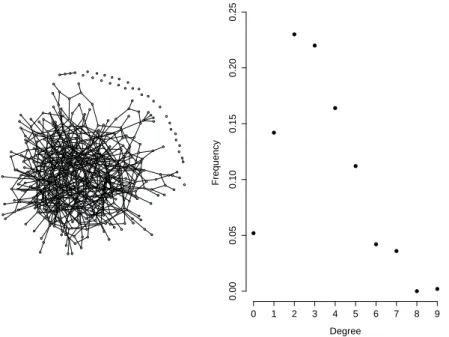
3.2 Node-link representation versus degree distribution representation of a network on 500 nodes. . . 32

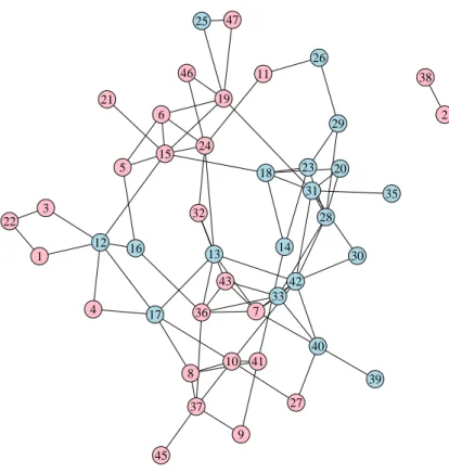
3.3 Network on 14 nodes . . . 35

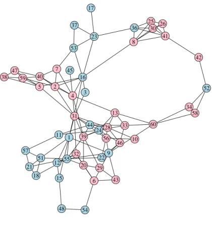
4.1 Social network for class 3A of Santo In´acio School, afternoon shift. . . 44

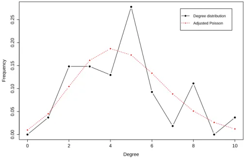
4.2 Degree distribution for the network depicted on figure 4.1. . . 45

A.1 Social network for class 3A of Salom´e Bastos School, morning shift. . . 60

A.2 Degree distribution for the network depicted on figure A.1. . . 60

A.3 Social network for class 3 of Luciano Feij˜ao School, morning shift. . . 61

A.5 Social network for class 3 of Luciano Feij˜ao School, afternoon shift. . . 62

A.7 Social network for class 3B of Jos´e de Alencar School, morning shift. . . 63

A.9 Social network for class 3F of Jos´e de Alencar School, afternoon shift. . . 64

A.11 Social network for class 3D of Presidente Humberto Castelo Branco School, morning shift. . . 65

A.13 Social network for class 3E of Presidente Humberto Castelo Branco School, afternoon shift. . . 66

A.15 Social network for class 3E of Figueiredo Correia School, afternoon shift. . . . 67

A.17 Social network for class 3A of Figueiredo Correia School, morning shift. . . 68

A.19 Social network for class 3A of Liceu do Cear´a School, morning shift. . . 69

A.21 Social network for class 3A of Liceu do Cear´a School, afternoon shift. . . 70

(14)

A.23 Social network for class 3C of Dona Maria Am´alia Bezerra School, afternoon

shift. . . 71

A.25 Social network for class 3A of Dona Maria Am´alia Bezerra School, morning shift. . . 72

A.27 Social network for class 3B of Liceu de Caucaia School, morning shift. . . 73

A.29 Social network for class 3D of Liceu de Caucaia School, afternoon shift. . . 74

A.31 Social network for class 3A of Liceu de Caucaia School, morning shift. . . 75

A.33 Social network for class 3F of General Eudoro Correia School, afternoon shift. 76 A.34 Degree distribution for the network depicted on figure A.33. . . 76

A.35 Social network for class 3B of General Eudoro Correia School, morning shift. . 77

A.37 Social network for class 3D of General Eudoro Correia School, morning shift. . 78

(15)

List of Tables

4.1 Geographic distribution of the data in the PAEST. . . 42

4.2 Class summary. . . 42

4.3 Geographic distribution of the data in the sample. . . 43

(16)

(17)

1 Introduction

It is very common to think in macroeconomic, socioeconomic and demographic variables as shaping an individual and influencing his or her microeconomic outcomes, like criminal activity, educational and labor market outcomes. However, despite these variables play an important role, we can not ignore the fact that the behavior of our social contacts influences our own behavior. In many situations and in a variety of environments, not just social, but also financial, business and scientific ones, just to mention a few, our peers are influencing our behavior and this can change some outcomes that may arise from the interactions with them. Think about criminal efforts, smoking behavior and other social diseases, the adoption of a new technology by firms, the purchase of a new product by consumers, human capital decisions, R&D efforts, public goods provision, information gathering, consumption externalities, herd behavior, location decisions by companies, bankruptcy and foreclosure decisions, etc. All these are examples of variables that may be influenced by the economic agents peers’ own behavior regarding each of these variables.

A large literature has developed around the study of peer effects on individu-als outcomes, as we show in the next chapter. More recently, with the development of databases containing information about the connections among the individuals in the data, econometricians could use this information for better understanding the network effects. Patacchini e Zenou (2012) developed a model in which conformism plays an im-portant role in shaping the behavior of individuals, the local-average model. As we show in more details in chapter 5, an individual loses utility if he fails to conform with his or her peers. This way, he or she will try to get closer to the average behavior of his or her social contacts. We use their model to estimate the peer effects in the school environment on two different outcomes: the probability of doing an exam without being prepared and the probability of cheating in an exam.

(20)

information about more then 2000 students from 47 public and privite schools in three geographical regions of Cear´a, namely the state’s capital, Fortaleza, its metropolitan area and the state’s countryside.

In the chapter 2 we make a review of the literature of peer effects on a variety of outcomes, such as crime, education and labor market. As we show, the literature of peer effects can be divided in two distinct groups regarding the methodology, namely the literature of neighborhood effects and the literature of network effects. In the first, mainly because data limitation, authors suppose that all the individuals surrounding an agent in some environment, such as a school or a neighborhood, are able to influence this agent’s behavior. This assumption brings an identification problem to the estimation of peer effects in econometric models of neighborhood effects, known as reflection problem, as we discuss in more details in chapter 5. The literature of network effects arises with the recent development of databases including the social and economic connections existing among the individuals in the data, making possible the use of the tools of Social and Economic Network Theory for the analysis of peer effects. When the networks present some easily identifiable features, the identification problem is overcame, and econometricians can find the real size of the peer effects.

In chapter 3 we introduce some important tools of the Social Network Theory. We begin with the characterization of a network, which is composed by a set of agents, the set of all individuals in that network, and by a graph, which is represented by a special matrix called adjacency matrix. The adjacency matrix summaries the social or economic connections that exist in the network. Basically, each row and column in the adjacency matrix indexes an individual in the network in such a way that, when two individuals are socially connected, the entrance of the adjacency matrix representing the connection between these two individuals is equal to a positive value, and zero if they are not socially connected. After the characterization of a network, we introduce some important definitions in Network Theory, such as paths, walks, n-neighborhoods and degree distribution. Such definitions are specially important for the econometric modeling of network effects and for the conditions of identification of the peer effects, as you will see in chapter 5. We then turn attention to the called centrality measures, which measure how central an individual is in a network in terms of direct and indirect connections. We give special attention to the eigenvector related measures, that have an important relation with the econometric models of network effects, including the model used in this dissertation.

In chapter 4 we talk about the database used in this research work, the PAEST, showing the demographic and geographic distribution of the data among the three regions of Cear´a and between private and public schools. We also talk about networks in the database and introduce the graphical representation of the networks for each one of the

(21)

classes used in this work, as well as an associated measure called degree distribution.

In chapter 5 we present Patacchini e Zenou (2012)’s local-average model. We also discuss in more detail the reflection problem and why the use of networks overcome this identification problem. The advantage of econometric models of network effects over models of neighborhood effects is shown by Bramoull´e, Djebbari e Fortin (2009), which show that the reflection problem barely never arises when we use this approach for estimating peer effects. We then present the estimation of the local-average model for our dependent variables, the probability of doing an exam without being prepared and the probability of cheating in an exam.

(22)

(23)

2 Neighborhood and Network Effects

The literature of peer effects over individuals outcomes has followed two distinct lines concerning the agent’s reference group, the social group where each individual be-longs, which can be thought as his or her classmates, coworkers, acquaintances, residential neighbors, firms in a production chain, etc. Just to mention a few. Although both at-tempt to capture the effect of thesocial spaceover the agent’s behavior and, consequently, over the outcomes that may arrive from social or economic interactions, they are quite different in methodology. This way, the literature of peer effects can be divided into the literature of neighborhood effects and network effects, and why we make this distinction will become clear shortly.

The literature of neighborhood effects considers the reference group of an individ-ual simply as being symmetric over all individindivid-uals within the same social space. This way, the reference group of an individual in this work would be all the people in is his or her classroom. The reference group is thought as the set of “residential neighbors”. In such a way, for peer effects in crime, the reference group of a criminal may be all the people in the neighborhood he lives; for peer effects in firms production, it may be other firms in the same industrial district, regardless of being competitors or not, regardless of being connected by a production chain or not; for peer effects in education, the reference group is usually the set of classmates or schoolmates. The list goes on, but the idea is that an economic agent is influenced by the composition of his neighbors, and shocks in the composition of his or her neighborhood may change some outcome that arises from social or economic interactions.

The other strand of the literature of peer effects, the literature of network effects, takes into account the social connections that may exist among the individuals in the social space. It is reasonable that an individual in a social space, such as a classroom, do not interact with everyone in that space. Instead, he or she has a social relation with a subset of individuals in that classroom. In this setup, the reference group of each individual is different within the social space, unless they form a social structure called clique. This literature uses the tools os the social network theory, which we introduce in the chapter 3.

(24)

focusing on its division between neighborhood and network effects and talk about the weakness and strengthness of each approach. In the next section, we make a review of the literature of neighborhood effects. Then we review the literature of network effects.

2.1 Neighborhood Effects

The biggest limitation for the development os models that take into account the network structure existing in any social context was certainly the lack of datasets including the social connections among the individuals in the data. Just recently some datasets with information about who is socially connected to who among the individuals inside the survey were available, such as the Add Health - The National Longitudinal Study of Adolescent to Adult Health - in United States, and the PAEST - Pesquisa de Aspira¸c˜oes e Expectativas dos Estudantes Concludentes do Ensino M´edio - in Brazil. It was in that context that the literature of neighborhood effects has developed.

Although social interactions play an important role in how individuals shape their behavior, the neighborhood effects may arise from local shocks or through institutions in an individual’s residential neighborhood, as pointed out by Topa e Zenou (2015). For instance, the bankruptcy of a local industry, the presence of churches or NGOs in a given location, etc. For education, more qualified teachers or policies aiming to improve students outcomes may influence the educational achievements of all individuals in that social space. This way, we should also distinguish the neighborhood effects as arising from social interactions and from those shocks and institutions.

Another limitation of this approach to estimate the peer effects is that econome-tricians face an identification problem, specifically known in the literature of peer effects as the reflection problem, which we discuss in more details in chapter 5. As shown by Manski (1993), when individuals interact socially, they affect each other mutually, making difficult to identify the extension of the influence of an agent’s social contacts behavior over his own behavior.

A common problem for the analysis of peer effects we can face in both approaches is that individuals may sort into networks because the individuals in that network or neighborhood already have similar tastes or behave similarly. If it is not possible con-trolling for these similar tastes or behaviors, we must be sure that the network is formed randomly. This is possible analysing the degree distribution, which we discuss in more details in section 3.3. Basically, if we observe that the relative frequency of the number of connections in a network follows a Poisson distribution, then we can assume that the individuals in that network are sorted randomly. It is clear that we can not use this arti-fice when we do not have information about the network structure, making more difficult to justify the random sort of agents in a neighborhood.

(25)

Finally, as discussed before, the individuals in the same residential neighborhood may be exposed to local shocks or by local institutions that may be unobserved by the econometrician.

Before Manski (1993), most works focused on the effects of growing up in disad-vantaged neighborhoods over educational achievement, employment, and other indicators of social welfare. For example, Corcoran et al. (1989) investigate the effects of family and neighborhood background on men’s economic status. They have found the existence of substantial disadvantages in economic status for black men, men from lower-income families, and men from more welfare-dependent families or communities. In the same line, Brooks-Gunn et al. (1993) investigate the effects of neighborhood characteristics on the development of children and adolescents. They have found effects of the presence of affluent neighbors on Childhood IQ, teenage births, and school-leaving, even after the differences in the socioeconomic characteristics of families are adjusted for. These works and others before Manski (1993) usually use family and neighborhood attributes and, sometimes, mean outcomes in the social space analyzed. This bring a problem of identi-fication to their model, as we show in more details in chapter 5, which invalidates their findings. Basically, including mean outcomes of the individuals in a neighborhood makes impossible to separate the peer effects from exogenous effects.

As exposed by Topa e Zenou (2015), subsequent works on neighborhood effects have followed two strategies to overcome the problem of model identification. The first was the use of experimental and quasi-experimental approaches. Most of these works focus on immigrant refugees sorted into locations determined by local authorities and how the characteristics of this new environment affected them. and also the relocation of families from public housing projects in poor neighborhoods to low-poverty neighborhoods.

Popkin, Rosenbaum e Meaden (1993) study the effect of relocating black low-income families who were either former or current residents in public housing and moved to subsidized housing in Chicago and its suburban areas, a governmental program called Gautreaux program. The selection of participants was not random, but the sort of agents into city neighborhoods and suburban neighborhoods was based on the availability of units, therefore quasi-random. They have found that the participants of the program who moved to suburban areas were significantly more likely to find a job after the moving than the participants who moved to city areas, even among those who had never had a job before moving.

(26)

He argues that the majority of households that left high-rise public housing in response to the demolitions moved to neighborhoods and schools that closely resemble those they left. Contrary to the Gautreaux experiment, Jacob (2004) finds no evidence of any impact of the demolitions and subsequent relocations on student outcomes.

Oreopoulos (2003) studies the effect on long-run labor market outcomes of adults who were assigned, when young, to substantially different public housing projects in Toronto. Same as Jacob (2004), Oreopoulos (2003) finds no evidence of neighborhood effects in a variety of outcomes, including unemployment, mean earnings, income, and welfare participation. However family differences, as measured by sibling outcome corre-lations, account for up to 30% of the total variance in the income and wages.

Studies based on the Moving to Opportunity program (see Ludwig, Duncan e Hirschfield (2001), Kling, Ludwig e Katz (2005) and Kling, Liebman e Katz (2007)), or simply MTO program, usually find no neighborhood effects on economic outcomes. As explained by Topa e Zenou (2015), this was a large, randomized experiment in which participants volunteered for the study, and they were randomly assigned to one of three groups: a control group, a group receiving a housing voucher without any restrictions, and a third group receiving a voucher to move to a low-poverty neighborhood. The last two groups moved to neighborhoods with significantly lower poverty rates, less crime, and in which residents reported feeling safer. Unlike the evidence of no neighborhood effects on economic outcomes, the studies found a large and significant neighborhood effect on a variety of adult mental health measures. Ludwig et al. (2012) studied the effect of the MTO program 10 to 15 years later the participants have received the housing vouchers. Again, neighborhood effects are no significant for economic outcomes, nor for physical health. They were reported to be marginally significant for mental health and highly significant for subjective well-being.

Another set of studies has focused on the resettlement of refugees into new locations selected by the host country authorities, such as Edin, Fredriksson e Aslund (2003), Aslund et al. (2011) and Beaman (2012), among others. These studies have found a significant neighborhood effect on outcomes such as employment status, earnings and educational performance.

A second approach to the estimation of neighborhood effects is based on structural models of social interactions. As explained by Topa e Zenou (2015), these models generate stationary distributions with well-defined properties over space, like excess variance across locations, or positive spatial correlations. The parameters of these models can then be estimated by matching moments from the simulated spatial distribution generated by the model with their empirical counterparts from spatial data on neighborhoods or cities.

For neighborhood effects on crime, Glaeser, Sacerdote e Scheinkman (1996) try to explain the variance of crime rates in United States cities across time, where the propensity

(27)

of engagement in a crime is influenced by the individual’s neighbors. They create a model where social interactions create enough covariance across individuals to explain the high cross-city variance of crime rates. The model provides an index of social interactions which suggests that the amount of social interactions is highest in petty crimes, moderate in more serious crimes, and almost negligible in murder and rape.

Topa (2001) analyzes a structural model of transitions into and out of unem-ployment that explicitly incorporates local interactions and allows agents to exchange information about job openings to estimate the impact of local social interaction effects on employment outcomes. He found a significantly positive amount of social interactions across neighbouring tracts. The local spillovers are stronger for areas with less educated workers and higher fractions of minorities.

In the next section, we make a review of the literature of network effects. The models discussed next use the tools of social and economic network theory, which we discuss in more details in chapter 2.

2.2 Network Effects

An agent may be influenced in two opposite ways by his or her peers. Most commonly, individuals tend to follow his or her peers actions. We can observe this in smoking behavior, criminal efforts, R&D efforts, etc. Just to mention a few. On the other hand, economic agents may want to distance themselves from the behavior of their peers. Examples include local good provision and information gathering. As the peers influence is a two-way road, we call those situations of games of strategic complements

andgames of strategic substitutes, respectively. Most of social and economic situations are based on complementarity, therefore, we will only discuss here the literature of network effects on games of strategic complements. We discuss in more details games of strategic complements in chapter 5, specifically the local-average model.

There are two different models of games of strategic complements, the local-aggregate model (see Calv´o-Armengol e Zenou (2004) and Ballester, Calv´o-Armengol e

Zenou (2006, 2010).) and the local-average model (see Patacchini e Zenou (2012).). In the first one, individuals are assumed to be influenced by the sum of social or economic contacts he or she has. In the local-average model, we suppose that an individual is influenced by the average behavior of his or her peers, here thought as the people here or she is connected, making a distinction in relation to the residential neighborhood in the literature of neighborhood effects.

(28)

we can easily differentiate the peer effects from the exogenous effects. In the literature of neighborhood effects, we consider that the reference group is symmetric among the indi-viduals in a social space, mainly due to limitations in datasets, and Manski (1993) shows that this setup brings the reflection problem, making impossible to separately identify the peer effects and the exogenous effects.

Patacchini e Zenou (2012) develop the local-average model, which we discuss in more details in section 5.2. According to their model, when interacting socially or eco-nomically, individuals gain utility when they conform to the average behavior of their social contacts. They study the criminal behavior of adolescents on a variety of crimes using the Add Health dataset, which contains information about the social connections among the individuals in the data, allowing the use of social network theory. They find that conformity plays an important role for all crimes, especially for petty crimes. This suggests that, for juvenile crime, an effective policy should be measured not only by the possible crime reduction it implies but also by the group interactions it engenders.

(29)

3 A Short Introduction to Network

Analysis

In this chapter, we introduce the analytical tools on how to represent and measure networks. An important feature of networks is about the positions individuals occupy in a network and how they influence and are influenced by their neighbors and indirect neighbors, or “the friends of my friends”. Some measures of clustering and centrality are introduced later in this chapter, and provide a great perspective of how important they can be for the microeconomic analysis of individuals outcomes. Now, we begin with some definitions on how to represent networks and formalize the notion of players, connections and indirect connections in a network.

3.1 How to Represent a Network

The most important components of a network are the players and the relations that may exist between them. Therefore, it is really important to represent these players and their possible relations in a tractable way, that can easily represent the network structure and be used in a broad class of applications. As it follows, we present basic concepts and definitions that help on the analysis of networks and that will eventually be used in this work. For further explanations on how to represent and measure networks, see Jackson (2010).

As we said, the main components of a network are the players and their possible relations. The players, or nodes, as will become clear later, might be any economic agent, like firms, governments, politicians, organizations, web pages, etc. Not just people. In a particular network, the nodes that are involved in this net of relationships will be represented by a set, as follows:

Definition 3.1. Let 1,· · · , n index the players that are involved in the network under analysis. The set of nodes,N, is given by N ={1, ..., n}.

(30)

or not. However, there are cases where one player relates to the other but this second does not relate to the first. In this case, where there is not a mutual connection between the players, we say that this kind of relation is a directed relationship. If at least one node in the set N does not have a mutual connection with some other node, we say that the network of then players is a directed network. If it is not the case, we have an undirected network.

Undirected networks are a common form of representing networks that involve friendships and partnerships, the central issue of this dissertation. The distinction between directed and undirected networks are not just conceptual. The ways researchers can model directed and undirected networks are quite different, so, depending on how connections between the players are formed, this distinction could be extremely important. Therefore, all the following definitions and network measures are assumed an undirected network set up. For the same review on directed networks, see Jackson (2010).

The relations among the n nodes in the set of nodes, N, can be summarized by the following matrix:

Definition 3.2. Let g a real-valued n×n matrix. The relation between the node i and the nodej is given by gij, wheregij = 1 if node i relates to node j, or gij = 0 otherwise.

In the case of undirected networks, it is always the case in whichgij =gji for all i andj inN, such thatg is as symmetric matrix, because the need of a mutual relationship between the players. g is often referred to as the adjacency matrix. The values of gii, the self-links or loops, may be 0 or 1, depending on the the situation under analysis.

Definition 3.3. A network, or graph, (N, g), consists of the set of nodes, N ={1, ..., n}, and then×n real-valued adjacency matrix, g.

An alternative way of describing the links between the nodes in a network (N, g) is to define g as a set of the existing links, g = {ij : gij = 1}. If the nodes i and j are linked to each other, we say that ij ∈ g. If they are not, we say that ij /∈ g. Saying that ij ∈g is equivalent to say that gij = 1. Seeing g as the adjacency matrix defined as Definition 3.2 or as a set of the existing links is just a matter of convenience, and they can alternate in this text, depending on the situation.

For instance, suppose a network involving 5 nodes, N = {1,2,3,4,5}, and adja-cency matrix given by

(31)

Figure 3.1: Network on 5 nodes

1

2 ₃

4

5

Prepared by the author.

g =



      

0 1 0 0 0 1 0 1 1 0 0 1 0 0 0 0 1 0 0 0 0 0 0 0 0



      

This network is depicted in figure 3.1, where the circles, or nodes, represent the players, and the straight lines, or links, represent an existing relationship between the two nodes connected by the link. The absence of a link between any two nodes indicates that these nodes do not relate to each other.

3.2 Some Important Definitions

(32)

Definition 3.4. A path in a network (N, g) between nodes iand j is a sequence of links

i1i2, ..., iK−1iK such that ikik+1 ∈ g for each k ∈ {1, ..., K −1}, with i1 = i and iK =j, and such that the sequencei1, ..., iK is distinct.

Definition 3.5. A walk in a network (N, g) between nodes i and j is a sequence of links

i1i2, ..., iK−1iK such thatikik+1 ∈g for each k ∈ {1, ..., K−1}, with i1 =i and iK =j.

The distinction between a path and a walk in a network is that a path involves only “handshakes” that have never occurred before, while in a walk, when trying to get in the terminal node, repeated interactions may occur.

Definition 3.6. A geodesic between nodes i and j is the shortest path between these nodes.

Sometimes, there are multiple ways to get in a person that is not direct connected to a node. The definition of geodesic is of a huge importance, because it is more likely that the indirect interactions between any two nodes occur via the shortest path between them.

It is easy to see that, if we set the self-linksgii= 0, the entrance gijk of the matrix

gk_{, the} _kth _{power of} _g_{, tells us how many walks of size} _k _{there exist between the nodes}

i and j in the network (N, g). This is actually one of the possible ways of solving the famous mathematical problem of the seven bridges of K¨onigsberg.

It is also important to consider the set of nodes in the network an individual is directly connected to, or the set of nodes one can reach through a given number of “handshakes”. It arises, then, the concept of neighborhood and extended neighborhoods.

Definition 3.7. The neighborhood of a node i,Ni(g), is the set of nodes thati is linked to. Ni(g) ={j :gij = 1}.

Given a set of nodes S ⊂N, the neighborhood of S is the union of the neighbor-hoods of the nodes inS:

NS(g) =

[

i∈S

Ni(g) ={j :∃i∈S, gij = 1}

The “friends and friends of my friends” set, or the extended neighborhood of size 2, which includes the nodesiis directly connected to and all the nodes that can be reached by paths of size 2, is given by:

N_i2(g) = Ni(g)∪



 [

j∈Ni(g)

Nj(g)





(33)

And, the k-neighborhood ofi, which consists of all nodes that can be reached from

i by paths of size less or equal than k, is given by:

N_ik(g) =Ni(g)∪



 [

j∈Ni(g)

N_jk−1(g)





Definition 3.8. Thedegree of a nodeiis the number of nodes that are directly connected to it. di(g) = #{j :gij = 1}= #Ni(g).

Finally, we define network density.

Definition 3.9. The density, d(g), of a network (N, g), describes the portion of the potential connections in a network that are actual connections, and may be calculated by:

d(g) =

Pn

i=1di(g)/n

n−1

So far, we have shown several tools on how to represent a network. On the next three sections, we begin the discussion on how to measure a network, beginning with the description of the degree distribution of networks and then introducing an overall measure of clustering, that enables us to compare networks regarding its cohesiveness, the clustering measure We finish with some microeconomic measures, that explicit the role of the centrality of a node on networks, the centrality measures.

3.3 Degree Distribution

An useful way of representing a network is through its degree distribution, which summary the relative frequencies of nodes’s degree. Large networks with hundreds or thousands of individuals are better represented on its degree distribution, as you can see on the network on 500 nodes depicted on figure 3.2.

Beyond this advantage regarding representation, the degree distribution also pro-vides us with some insights about the network formation and growing process. The degree distribution on the right side of figure 3.2 is a typical example of the degree distribution of a network formed under a Poisson distribution, which it is due to Erdos e Renyi (1959) and we shortly introduce next.

3.3.1 Poisson Distribution

(34)

Figure 3.2: Node-link representation versus degree distribution representation of a net-work on 500 nodes.

0 1 2 3 4 5 6 7 8 9

0.00

0.05

0.10

0.15

0.20

0.25

Degree

Frequency

such that a whole network is formed with probability given by a binomial distribution. Any network onn nodes with x links, where 0≤x≤ n−1₂

, has a probability of forming given by:

px₍₁₋_p₎₍n−1

2 )−x

With this completely random process of link formation given by a Bernoulli dis-tribution, the degree distribution can easily be derived from the statistical theory. The degree distribution gives us the probability that any given node has a degree of d. Each node can be linked to n−1 other nodes, so, the probability of having a degree of d is given by:

f(d) =

n−1

d

pd(1−p)(n−1)−d (3.1)

When (n−1)p−→0, the binomial distribution on 3.1 can be approximated by a Poisson distribution. The Poisson degree distribution is given by:

f(p) = e −λ_λd

d!

whereλ = (n−1)p.

(35)

When links on a network are formed randomly with a fixed probability of link formation, we say that this network is a Poisson random network. The degree differences across nodes are due to a uniformly random noise on the number os links a node may has.

3.3.2 Power Distribution

The power distribution is given by the following density:

f(d) = cd−γ (3.2)

where c and γ are parameters of this distribution.

Differently from the Poisson distribution, the differences on nodes’ degree arise from a cumulative process in which nodes gain connections proportionally to its current degree, such that nodes with a high degree gain connections much faster than low degree nodes. We call this process of “rich-get-richer” process.

When looking to degree distributions of networks, its usual to see fat tails when a network exhibits this process of link formation, because of the high number of low degree nodes. It is also useful to take the logarithm of both degree and its relative frequency, such that we would see a linear relation between the logarithm of degree and the logarithm of its relative frequency1_.

3.4 Clustering Measures

The spread of information or other benefits, as well as harmful things, is much faster when a network is closely-knit. Measures that are able to capture this aspect of cohesiveness in networks have its importance, because enable us to compare different net-works in terms of their information transmission. Here, we introduce a way of measuring how clustered networks are.

In a network, the most clustered group possibly would be that in which all its members are connected to each other. We call this kind of cluster of clique. A clique is a set of nodes S ⊂N such that all nodes in S are connected to each other. Conceptually, we consider a clique a set with at least three nodes, otherwise, any two nodes connected could be a clique.

A simple way of calculating this aspect of cliquishness is looking to all nodes connected to a node i and verify, among all possible pairs, what fraction of them are also connected to each other. For instance, if ij and ik ∈ g, in what fraction does jk ∈ g?

1

(36)

This gives us an idea of the relative number of cliques of size three there exist in the network. Hence, the overall clustering is given by:

Cl(g) =

P

i#{jk ∈g|k 6=j, j ∈Ni(g), k∈Ni(g)}

P

i#{jk|k6=j, j ∈Ni(g), k ∈Ni(g)} =

P

i;j6=i;k6=j;k6=igijgikgjk

P

i;j6=i;k6=j;k6=igijgik

The overall clustering ranges from 0 to 1. The closer to 1, more clustered a network is, meaning that most of the neighbors of a node are also neighbors.

Next, we introduce some measures that capture an important characteristic of the nodes, the centrality. How central are the nodes in a network and how this influence things like information flows, bargaining power, the spread of diseases, and a sort of other outcomes that may be influenced by a node’s centrality.

3.5 Centrality Measures

In the last section, we showed a measure of clustering, that is able to capture an overall aspect of a network. However, we may be interested in microeconomic measures, that capture the influence of the network in the nodes’ outcomes. How the neighborhood of a node influence his or her outcomes. Hence, measures that capture how central an individual is in a network can bring great insights about how his or her outcomes are influenced, other than just the economic and sociodemographic environments.

These centrality measures can be categorized into for different groups, and we introduce them next.

3.5.1 Degree Centrality

The degree centrality tells us how connected a node is in the network. Suppose an individual node in a network (N, g) that is directly linked to all the othern−1 nodes. This individual is quite central in this network, because he can reach every single node directly, without the need of any intermediary. On the other hand, a node linked to only one node on the pool o n nodes is not very central. He always need the node he is connected to for reaching any other node.

A simple way of keeping track the centrality of the nodes is look to the fraction of the nodes he is connected to among all then−1 nodes he can potentially be connected to. According to Definition 3.8, the number of nodes an individual is connected to is given by its degree. So, thedegree centrality of a node i can be calculated by:

CeD_i (g) = di(g)

n−1

(37)

Figure 3.3: Network on 14 nodes

1 2 3

4 5

6 7 8

9 10 11 12 13

14

The degree centrality ranges from 0 to 1. When CeD

i (g) = 0, node i is not connected to any other node. On the other hand, when CeD

i (g) = 1, node i is connected to all the other n−1 nodes in the network.

The degree centrality has some limitations, limitations that make its use very restrictive. For illustrating these limitations, suppose the network depicted in figure 3.3. Observe nodes 2 and 12. Node 2 has a degree centrality of 0.0769, while node 12 has a degree centrality of 0.2367, which means that they are connected to 7.69% and 23.67% of all nodes they could be connected to, respectively. However, node 2 is connected to node 1, which has the larger degree centrality, 0.6153, while node 12 is connected to nodes with a much lower degree centrality, 0.1538, 0.0769 and 0.0769 for nodes 11, 13 and 14, respectively. It is easy to see that node 2 is more likely to reach other nodes in the network through indirect connections, because he has a immediate connection with the node with more connections on the network. Although the node that has only one connection is more likely to reach other nodes in the network through indirect connections, the degree centrality for him does not capture this feature. Other centrality measures are needed in order to capture this aspect.

3.5.2 Closeness Centrality

(38)

looking only to the number of nodes an individual is connected to, here we consider the whole network and how central a node is considering their direct and indirect connections.

Letl(i, j) the number of links on the geodesic2 _between _i _and _j_{. Averaging} _l₍_{i, j}₎ overj we have a measure that captures the average path distance between node iand all the other nodes. The bigger it is, the bigger the overall distance from node i to all the other nodes, therefore, less central. It is usual to take the inverse of this measure, such that bigger values mean more centrality:

CeC_i (g) = Pn−1

j6=il(i, j)

This measure ranges from 0 to 1. Even in networks with large diameters3_{, and,} because of this, a particular node may have a large average distance, when we take the inverse, this distance get closer to 0. On the other side, the least average distance possible is 1, which means that a node is directly connected to all the other nodes in the network. When we take the inverse of the average distance, this node remains with 1 as closeness centrality.

For the network depicted in figure 3.3, the closeness centrality for nodes 2 and 12 is 0.3333 and 0.2766, respectively, which confirms our suspicious that node 2 was more likely than node 12 to reach other nodes through indirect connections, and shows that the closeness centrality overcome the limitations that arise from the use of degree centrality.

Although the average path distance attain to the task of capturing all of the neighborhood effect of a network on an individual, it weights equally nodes that are far away from the individual and nodes directly connected to it. A particular measure that overcome this problem is the decay centrality. Consider a decay parameter δ, such that 0< δ < 1. Setting l(i, j) = ∞ for nodes that are not path connected with i, the decay centrality,

Cede_i (g) = X j6=i

δl(i,j)

gives more weight for nodes that are closer to the individual, and weight zero for nodes not path connected.

3.5.3 Betweenness Centrality

As the name suggests, the betweenness centrality measures are based on how important a node is in order to connect two distinct nodes. Indirect connections are just

2

See definition 3.6. 3

The largest distance between any two nodes.

(39)

attainable if it is possible to get in the terminal node by the intermediation of all the nodes that are between the two individuals. If one of these intermediary nodes are not willing to make this intermediation, the indirect connection will not occur.

The first to see the importance of how well situated a node is in terms of interme-diate indirect connections was Freeman (1977), and I introduce his betweenness centrality measure next.

Let Pi(kj) the number of geodesics between k and j that goes through i, and

P(kj) the whole number of geodesics between k and j. Pi(kj)/P(kj) gives us an idea on how important node i is in connectingk and j. If it is close to 0, iis not very important in connecting the two nodes. It lies in a few paths that connect k and j, so it is unlikely he will be contacted for intermediating the connection. On the other hand, if it is equal to 1, he is always needed for making the connection happen, and, therefore, more central. Averaging Pi(kj)/P(kj) over all combinations of k and j provides an idea on the overall importance of iin connecting the network. Freeman’s measure is given by:

CeB_i (g) = X k6=j:i /∈{k,j}

Pi(kj)/P(kj) n−1

2

For the network depicted on figure 3.3, the node with larger betweenness centrality is node one, 0.8076, which means that it lies on 80,76% of all shortest paths on the network he or she belongs. Nodes 2, 3, 4, 5, 6, 7, 8, 13 and 14 have a betweenness centrality of 0, which means that they are never asked to intermediate any indirect connection.

3.5.4 Eigenvector Related Centrality Measures

Eigenvector centrality measures relies on the premise that a node’s importance is determined by its neighbors’ importance. A first approach to this issue was made by Katz (1953).

The Katz prestige of a node i, Pk

i (g), is the sum of the prestige, or centrality, of its neighbors, weighted by theirs respective degrees:

P_ik(g) =X j6=i

gij

Pk j(g)

dj(g)

(3.3)

(40)

Considering all the n nodes in a network (N, g), we have the following system for the Katz prestige measure defined in 3.3:

P₁k(g) = g12

d2(g)P k

2(g) +· · ·+

g1n

dn(g)P k n(g)

P₂k(g) = g21

d1(g)P k

1(g) +· · ·+

g2n

dn(g)P k n(g)

... (3.4)

P_nk(g) = g1n

d1(g)

P₁k(g) +· · ·+ gn−1,n

dn−1(g)

P_n−1k (g)

If we set the self-links gii = 0, we can write the system of equations in 3.4 in the matrix form as follows:

Pk(g) = ˆgPk(g) (3.5)

Where Pk(g) is a n×1 column vector and ˆg a n×n matrix.

Observe that, in order to calculate the Katz prestige measure in 3.5, we need just to find the eigenvector Pk₍_g_{) belonging to the unit eigenvalue.}

Following Katz (1953), Bonacich (1972) proposes a centrality measure that does not normalize the adjacency matrix by the nodes’ degree. His measure, known as eigen-vector centrality, uses the idea that the centrality of a node is proportional to the sum of the centrality of its neighbors:

C_ie(g) = 1

λ

X

j6=i

gijCje(g)

Again, letting the self-links gii= 0, we have the following system in matrix form:

λCe(g) =gCe(g) (3.6)

Like in the Katz prestige measure, finding the eigenvector centrality measure in 3.6 is a simple task of calculating the eigenvector Ce₍_g_{) belonging to the eigenvalue} _λ_{. It} is a convention to look for the the eigenvector associated with the largest eigenvalue.

Katz (1953) also introduce a measure of centrality that covers the idea of the power of indirect connections. Remember from section 3.1 that a way of keeping track of how many walks of size k there exist between two distinct nodes is to look to the kth _power of the adjacency matrix. Defining a, such that 0< a < 1, we can look to the centrality of a node as the weighted sum of the walks that it has emanating from it. More distant nodes receive less weight. The second Katz prestige measure is given by:

(41)

PK2(g, a) =agI+a2g2I+a3g3I+· · ·

= (1 +ag+a2g2+· · ·)agI

= (I−ag)−1agI

Bonacich (1987) extends the second Katz prestige measure as follows:

CeB(g, a, b) = (I−bg)−1agI (3.7)

(42)

(43)

4 Database

The database used in this research was the PAEST − Pesquisa de Aspira¸cões e Expectativas dos Estudantes Concludentes do Ensino Médio − or Survey on Aspirations and Expectations of High School Students. The PAEST collected detailed information about the context students face in their last year of high school. It has information about family structure, socio-demographics, educational achievement and performance, networks through family and friends, sources and quality of information about undergrad-uate studies and expectations about labor market and educational choices of students in the third grade of high school in the northwestern state of Ceará, in Brazil.

Before talking about the demographic and geographic distribution of the data, it worths to comment about the sample unit in PAEST. The smallest sample unit in the PAEST is, indeed, the student. However, like in the American database Add Health, used in Patacchini e Zenou (2012) for the same purpose as ours, the PAEST has also information about the network structure existing in each classroom the student sampled belongs, allowing us to use models of network effects to study peer effects over educational outcomes, which makes it possible to distinguish the peer effects from the exogenous effects, as shown by Bramoull´e, Djebbari e Fortin (2009). This way, the classroom is also the sample unit in the PAEST.

Schools in the cities of Fortaleza, Caucaia, Maracanaú, Eusébio, Sobral, Juazeiro do Norte and Crato, composing three distinct geographical groups, to know, the state’s capital (Fortaleza), the Metropoliotan Area of Fortaleza (Caucaia, Maracanaú and Eusébio) and the state’s countryside (Sobral, Juazeiro do Norte and Crato), were sampled according to their demographic distribution in the state of Ceará.

(44)

Table 4.1: Geographic distribution of the data in the PAEST.

Region Private school Public school Total

Fortaleza 244 807 1,051

Metropolitan Area of Fortaleza 79 525 604

Cear´a countryside 189 498 687

TOTAL 512 1,830 2,342

Table 4.2: Class summary.

School name School type Shift Class name

1 Santo In´acio Private Afternoon 3A

2 Presidente Humberto Castelo Branco Public Morning 3D 3 Presidente Humberto Castelo Branco Public Afternoon 3E

4 Liceu do Cear´a Public Afternoon 3A

5 Liceu do Cear´a Public Morning 3A

6 Figueiredo Correia Public Morning 3A

7 Figueiredo Correia Public Afternoon 3E

8 Salome Bastos Private Morning 3A

9 Jos´e de Alencar Public Morning 3B

10 Jos´e de Alencar Public Afternoon 3F

11 Col´egio Luciano Feij˜ao Private Afternoon 3

12 Col´egio Luciano Feij˜ao Private Morning 3

13 EEFM Dona Maria Amalia Bezerra Public Afternoon 3C 14 EEFM Dona Maria Amalia Bezerra Public Morning 3A

15 General Eudoro Correia Public Morning 3B

16 General Eudoro Correia Public Morning 3D

17 General Eudoro Correia Public Afternoon 3F

18 Liceu de Caucaia Public Morning 3A

19 Liceu de Caucaia Public Morning 3B

20 Liceu de Caucaia Public Afternoon 3D

composition of the population. The data is also stratified into morning and afternoon shifts, since most schools in Brazil have these two distinct shifts, with no differences regarding syllabus. In such a way, the data can account for possible differences between students in the two shifts.

Altogether, students and their respective classes from 36 public schools and 11 private schools were sampled, with at least one class in each shift being interviewed, whenever possible. Just in small number of cases either one class or more than two classes in a same school were sampled. The final number of students sampled by the PAEST, divided according geographical region and school type is given in table 4.1.

For this research, a subset of 20 classes from the PAEST were made available. The

(45)

Table 4.3: Geographic distribution of the data in the sample.

Region Private school Public school Total

Fortaleza 68 213 281

Metropolitan Area of Fortaleza 0 94 94

Cear´a countryside 64 80 144

TOTAL 132 387 519

20 classes came from 10 schools, being 7 public schools and 3 private schools. Each class, with school name, school type, shift and class name is given in table 4.2. Our sample is composed by 519 students from all the three geographical regions of Cear´a. The exact stratification of the sample used in this research is given in table 4.3.

4.1 Networks in PAEST

The PAEST asks each student to list up to five other students in his classroom as his friends. Not always, when a student lists other as his or her friend, this second one lists the first. As some students were absent or refused to participate in the PAEST, a student can also list someone who was not interviewed, but who is part of the network.

In this work, we will consider that, when a student lists other as his friend, there is a mutual relationship between them, even if the second one has not listed the first. In other words, the networks are undirected. Other assumptions can be made about the the nature of the relationships in the networks. We can consider the networks as being directed or give more weight for links in which students list each other. The assumption o undirected network, however, seems to make more sense than the assumption of directed network, since it is very unlike that the information flow has only one direction in networks of friendship.

(46)

Figure 4.1: Social network for class 3A of Santo In´acio School, afternoon shift. 31 60 25 56 5 8 20 40 21 39 18 22 13 52 59 54 51 24 9 4 15 23 47 2 44 11 12 57 6 36 55 33 28 32 7 41 53 30 43 16 1 29 58 48 26 10 38 42 37 3 34 17 46 45

(47)

Figure 4.2: Degree distribution for the network depicted on figure 4.1.

0 2 4 6 8 10

0.00

0.05

0.10

0.15

0.20

0.25

Degree

Frequency

Degree distribution Adjusted Poisson

(48)

(49)

5 Econometric Model

When economists or sociologists try to study the effects of social contacts over individuals’ outcomes, or, in other words, peer effects, it is usual to approach this issue including in the econometric model a broad measure summarizing the neighborhood char-acteristics1_{, usually an average of the characteristics of all individuals living or interacting} in a same environment.

However, as shown by Manski (1993), this approach has a serious problem of iden-tification, known in the literature as the reflection problem. Think about an individual’s outcome as a personal choice of effort in exerting some activity. His choice of effort de-pends on some of his observable characteristics, and also may dede-pends on the choices of effort of his social contacts. As an individual’s choice of effort depends on his observable characteristics, the peers’ choices of effort also depend on their observable characteristics. Hence, we have to differentiate between the effect of peers’ choice of effort, or the endoge-nous peer effects, and peers’ characteristics that do impact on their choice of effort, or the exogenous contextual effects. When the reference group, the group in which each in-dividual belongs, is the same for all inin-dividuals, it is impossible to separately identify the endogenous peer effect and the exogenous contextual effect. For illustrating this, suppose the standard peer-effect model, the linear-in-means model, described as following:

yi,r=φE(yr) +γE(xr) +βxi,r+εi,r (5.1)

where yi,r is the outcome of individual i belonging to the reference group r, that arises from some social interaction, (like a GPA, number of criminal activities, etc.), E(yr) the average of outcome y among all individuals in the reference group r, xi,r an observable characteristic, or a vector of observable characteristics, of individual i in the reference group r (like gender, income, age, educational level, etc.), E(xr) denotes the average of the observable characteristics of all individuals belonging to reference group r, and εi,r an stochastic error term. The parameters φ and γ represent the endogenous peer effect and the exogenous contextual effect, respectively. As we said the reference group r is the

1

(50)

same for all individuals, so, the reference group of an individual in our data set would be his whole class, disregarding the network structure that, indeed, exist.

We show next that it is impossible to identify the endogenous peer effect, φ, and separate it from the contextual exogenous effect, γ. Let E(εi,r|yr, xr) = 0. Taking the conditional expectation on both sides of equation 5.1 and solving the resulting expression forE(yr), we have:

E(yr) =

γ+β

1−φ

E(xr) (5.2)

Replacing 5.2 on 5.1 yields:

yi,r =

φ(γ +β) +γ(1−φ) 1−φ

E(xr) +βx+i, r+εi,r (5.3)

As you can see on equations 5.1 and 5.3, there are more structural parameters than parameters in the reduced form in 5.3, and it is not possible to separately identify the endogenous peer effect and the exogenous contextual effect.

Identifying the endogenous peer effect is an important task not just in a empirical and technical point of view, but also because of its social multiplier effect, the multiplying power that some policy aiming an individual has to spread over this individual’s peers and his indirect contacts. For illustrating this, consider an educational program targeting criminal individuals. An individual affected by this policy may stop his criminal activities, and then he can influence his peers to reduce, or even stop, their criminal activities, and then these individuals may influence their peers in the same way, and so forth. On the other side, policies affecting exogenous variables, like the gender composition of a classroom, will probably not have a social multiplier effect. Fortunately, with the use of the network structure is possible to work around the identification problem.

When the reference group is set as the social contacts of the individuals, or, in other words, when we take into account the network structure of a group of individuals, the reflection problem barely never arises, because the reference group of each agent is different, as shown by Bramoull´e, Djebbari e Fortin (2009).

Next, we introduce semi-anonymous graphical games, from where some of the econometric models of network effects, in special the local-average model, are derived, and then we present our empirical strategy for estimating the peer effects in our data set.

5.1 Semi-anonymous Graphical Games

In a social context, the decision for a player to take a given action may depend on the popularity of this action among his or her social or economic contacts. As an

(51)

example, think about smoking or criminal behavior, R&D efforts, the adoption of a new technology by firms, the allocation of time between study and leisure, etc. However, as the player influenced by the actions of his/her social contacts is also part of the social contacts of other players, his/her action also influence them. Hence, all these examples are also examples of strategic interactions, and, therefore, can be modeled by graphical games, in this case, by the called anonymous and semi-anonymous graphical games.

In a anonymous graphical game, the decision of a player to take a given action depends on the number of other players taking this same action in a symmetric way. His or her decision does not depend on who is taking the action. Differently, in a semi-anonymous graphical game, his or her decision in taking an action depends on the number of his direct contacts, or friends, taking the action.

There are two different classes of semi-anonymous graphical games, relatively to how the utility of taking or not an action changes with the number of friends taking this action. When the utility increases, we say that the strategic interaction is a game of

strategic complements, and includes most of the social and economic situations, like those cited above. On the other side, when the utility of taking an action decreases with the number of contacts taking the same action, the interaction is said to be a game ofstrategic substitutes, and encompass situations like the provision of a public good and information gathering (JACKSON, 2010). Next, we formally define games of strategic complements, since they encompass the relation we are modeling on this dissertation.

Definition 5.1. Letui(xi, m) :❘2+ −→❘a real-valued utility function, wherexi denotes the action of player i, with xi = 1 if the player is taking a given action and xi = 0 otherwise, andm the number of players inNi(g), the neighborhood of i, withxj = 1. Let

m > m′_{. A semi-anonymous graphical game exhibits} _{strategic complements} _{if it satisfies:}

ui(1, m)−udi(0, m)> ui(1, m

′₎₋_u_i(0_{, m}′₎

for all i∈N.

The model we introduce next, the local-average model, is an example of a semi-anonymous graphical game of strategic complements, since the utility of taking an action increases with the average sum of active links an individual has. In this model, the social multiplier is due to the average effort of a player’s friends in exerting some activity, like studying or committing a crime.

5.2 The Local-average Model

(52)

networks in our sample. On this game, each player decides the level of effort to exert in some activity. The level of effort of individuali in network r is denoted by yi,r. If we set the self-linksgii= 0, the utility function of player iin network r as function of his effort and the effort of his peers is given by:

ui,r(y_r, gr) = (a∗_i,r+η∗_r+ε∗_i,r)yi,r− 1 2y

2 i,r−

λ

2(yi,r−yi,r)

2 _(5.4)

where yr is an nr-dimensional vector of efforts. This utility function has two parts, an individual part and a part representing the local-average effect, given by the last term on the righthand side of equation 5.4. The terma∗

i,ris a measure that captures the observable characteristics of playeri(like gender, age, years of study, etc.) and the observable average characteristics of playeri’s direct contacts (like the fraction of male or female friends, their average age, their average years of study, etc.), and can be written as:

a∗_i,r= M

X

m=1

βmxmi,r+ 1

di(gr) M X m=1 nr X j=1

gij,rxmj,rγm

where xi,r = {x1

i,r, . . . , xMi,r} is a set of M variables for the observable characteristics of playeri, and βm and γm parameters associated to the variablesxmi,r andxmj,r, respectively. Back to the utility function in 5.4, η∗

r denotes the unobservable network characteristics, an unobserved heterogeneity among networks, andε∗

i,r a stochastic error term. On the local-average effect, given by

λ

2(yi,r−yi,r) 2

the termydenotes the average level of effort of player i’s social contacts, and is given by:

y_i,r = 1

di(gr) nr

X

j=1

gij,ryj,r = nr

X

j=1

g_ij,r∗ yj,r (5.5)

where di(gr) is the degree of player i in network r, as defined in definition 3.8, and

g∗

ij,r = gij,r/di(gr). The matrix with each entrance given by gij,r∗ , the matrix g∗r, is a row-normalization of the adjacency matrix gr.

The local-average effect captures how the choices of effort by player i’s social contacts influence player i’s own choices of effort. On equation 5.4, observe that the utility of player idecreases with his distance from the average level of effort of his social contacts. This way, each individual has as an objective to minimize the social distance between himself and his reference group. For instance, it is likely that an individual with low performance in mathematics in a group of individuals with high performance in the

(53)

subject will try to improve his performance to conform with his peers. Because of this, the parameter λ is sometimes called the taste for conformity. An individual loses utility if he does not conform to his social contacts.

Each player will choose a level of effort that maximizes his utility function. There-fore the Nash equilibrium in pure strategies for this graphical game, y∗

r ∈ ❘nr, satisfies, for all r and alli∈Nr:

y∗_i,r=φ

nr

X

j=1

g∗_ij,ry_j,r∗ +ai,r+ηr+εi,r (5.6)

where φ =λ/(1 +λ),ai,r =a∗i,r/(1 +λ),ηr =ηr∗/(1 +λ) and εi,r =ε∗i,r/(1 +λ).

It is possible to show that, if φ < 1, the system of best-reply functions in 5.6 has a unique solution, given by:

y∗_r = (Inr −φg

∗

r)−1αrgr∗Inr (5.7)

for r = 1, . . . , r. Where αr =ai,r+ηr+εi,r.

Observe that the Nash equilibrium on equation 5.7 is the same as the Bonacichi Centrality represented on equation 3.7. This way, the parameter φ captures how the benefit of being path-connected to someone decays with the distance between them.

5.2.1 Conditions for Identification of the Local-average Model

Differently from the linear-in-means model in equation 5.1, on the local-average model, each individual is influenced by his or her peers in a different way, since no one has the same reference group. Hence, each player is differently influenced by his/her peer’s choices for effort. In contrast, when the reference group is the same for all individuals, the peer effects are an externality that affects identically every individual in a neighborhood. Besides not being a plausible hypothesis, it presents empirical problems that make its use too restrictive. In this section, we explain why the use of network effects works around the identification problem, making its use ideal for finding endogenous peer effects.

Let ri the reference group of individual i on network r. Rewriting the linear-in-means model for the hypothesis of different reference groups and including a network unobservable heterogeneity, ηr, we have the following econometric model:

yi,ri =φE(yri) +γE(xri) +βxi,ri+ηr+εi,ri (5.8)

whereE(yri) =yi,r, as defined on equation 5.5, E(xri) denotes the average characteristics