ABSTRACT: This study compared the performance of ordinary kriging (OK) and regression krig-ing (RK) to predict soil physical-chemical properties in topsoil (0-15 cm). Mean prediction of error and root mean square of prediction error were used to assess the prediction methods. Two watersheds with contrasting soil-landscape features were studied, for which the prediction methods were performed differently. A multiple linear stepwise regression model was performed with RK using digital terrain models (DTMs) and remote sensing images in order to choose the best auxiliary covariates. Different pedogenic factors and land uses control soil property distribu-tions in each watershed, and soil properties often display contrasting scales of variability. Envi-ronmental covariables and predictive methods can be useful in one site study, but inappropriate in another one. A better linear correlation was found at Lavrinha Creek Watershed, suggesting a relationship between contemporaneous landforms and soil properties, and RK outperformed OK. In most cases, RK did not outperform OK at the Marcela Creek Watershed due to lack of linear correlation between covariates and soil properties. Since alternatives of simple OK have been sought, other prediction methods should also be tested, considering not only the linear relation-ships between covariate and soil properties, but also the systematic pattern of soil property distributions over that landscape.
Keywords: ordinary kriging, multiple linear regression, regression kriging 1Federal University of Lavras − Soil Science Dept., C.P.
3037 − 37200-000 − Lavras , MG – Brazil. 2Federal University of Lavras − Engineering Dept. 3Purdue University – Dept. of Agronomy, Lilly Hall of Life Sciences, 915, W. State Street − 47906, West Lafayette, IN − USA.
*Corresponding author <[email protected]>
Edited by: Silvia del Carmen Imhoff
Spatial prediction of soil properties in two contrasting physiographic regions in Brazil
Michele Duarte de Menezes1, Sérgio Henrique Godinho Silva1, Carlos Rogério de Mello2, Phillip Ray Owens3, Nilton Curi1*
Received February 20, 2015 Accepted September 01, 2015
Introduction
Geostatistic techniques can estimate soil proper-ties at unsampled locations, providing valuable infor-mation for precision agriculture and environmental studies. Ordinary kriging (OK) is a spatial interpolation technique that depends on a weighting scheme dictated by the variogram, where closer sample locations have greater impact on the final prediction (Bishop and Mc-Bratney, 2001). One advantage of OK is its simplicity of use and is included in most software packages (Hengl et al., 2007).
As OK uses only observed data to map unsampled areas, more recent innovations have been preferred, such as hybrid geostatistical procedures. These techniques ac-count for environmental correlation, and often result in more accurate local predictions (Goovaerts, 1999; Mc-Bratney et al., 2000). One example is the regression krig-ing (RK), in which the interpolation is not only based on observed data, but also on the spatial structure of residu-als from regression of the target variable on spatially ex-haustive auxiliary variables (raster based mainly) (Hengl et al., 2007).
The auxiliary variables or environmental covari-ates use concepts of soil forming factors equation in the CLORPT (Jenny, 1941) and SCORPAN models (McBrat-ney et al., 2003). In these S: soil or other properties of the soil at a point; C: climate; O: organisms, vegetation, fauna or human activity; R: topography or landscape at-tributes; P: parent material or lithology; A: age, the time factor; N: space, spatial location. The terrain attributes are the main covariates used due to the strong relation-ship between relief and soil features (Jenny, 1941; Grun-wald, 2009).
Many studies have demonstrated that RK per-forms better than OK, cokriging or multiple regressions (Herbst et al., 2006; Odeh et al., 1995; Sumfleth and Duttmann, 2008; Zhu and Lin, 2010), even when only poorly correlated covariates are available (Bishop and McBratney, 2001). Simple linear regression modeling is most commonly used to model soil data. However, the relationship between soil and auxiliary variables is not necessarily linear, and could be unknown and often very noisy (Hengl et al., 2004).
This study had as objective the comparison of OK and RK for predicting soil physical and chemical proper-ties, in different physiographic regions in Minas Gerais State, Brazil. Predictive methods and environmental co-variables present different performances, since different pedogenic factors or land use control the soil property distributions. The hypothesis of this work is that the re-lationships between terrain attributes and soil properties are stronger in relatively young landscapes, so that RK would perform better than OK.
Materials and Methods
The study sites
Mantiqueira Range region (LCW) and Campo das Ver-tentes region (MCW). Additional characteristics of study sites are listed in the Table 1.
LCW is a headwater watershed located in the Mantiqueira Range Region. Its parent material is a gneiss from the Neoproterozoic, whose alteration re-sulted in the predominance of Inceptsols with moderate developement and well drained soil classes. The relief is steep with concave-convex hillsides, predominance of linear pedoforms, and narrow fluvial plains. Hydromor-phic soils occupy the toeslope positions, where the water table is near to the surface most of the year (Menezes et al., 2014; Silva et al., 2014).
MCW is located in the Campos das Vertentes Pla-teau geomorphological unit where erosion has intensely dissected this geomorphological plateau and the result-ing forms were described as landforms of homogeneous dissection . The parent material is micachist and phyllite from the Proterozoic. The relief is represented by gentle slopes with intense soil weathering, where Oxisols is the most extensive soil class.
Soil sampling and analysis
The topsoil (0-15 cm) was sampled at both water-sheds. A total of 198 points were sampled at LCW, fol-lowing the regular grids 300 × 300 m and refined scale 60 × 60 m and 20 × 20 m, and two transects with the distance of 20 m between points (a total of 54 and 14 sampled points per transect). A total of 165 points were
sampled at MCW, following the regular grids 240 × 240 m and refined scale 60 × 60 m. The sampling in the refined scale was conducted to capture the high spatial variability of physical and chemical properties at the finer scale. Sampling scheme at small scale also enables to gain confidence about the variogram behavior at short distances and thus, reduces nugget effect. The land use and soil classes were criteria used for choosing places with refined scale which would likely correspond to ar-eas where soil properties are likely to have greater vari-ability. The sampling scheme is presented in the Figure 2.
In order to create one independent validation data set to evaluate the performance of prediction methods, the total data set was divided into training and valida-tion sets. Of the total number of soils sampled, 25 points were used as validation points at LCW and 20 points at MCW which accounts for 12 % of the total samples for each watershed. The validation data set was randomly chosen and not used in the models to develop predic-tions.
Soil properties determined were bulk density by the volumetric ring method (EMBRAPA, 1997); or-ganic matter according to Walkley and Black (1934); drainable porosity calculated by the difference be-tween saturation water content and soil water con-tent at field capacity; saturated hydraulic conductivity (Ksat) determined in situ through constant flow per-meameter; and total porosity calculated according to the equation:
Total porosity bulk density
particle density
% *
( )
= −
100 1
where: particle density was determined by the volumet-ric flask method (EMBRAPA, 1997).
Environmental covariates
When climate, parent material, and time are rela-tively constant, the topography and organisms would be the greatest driver of soil differentiation (Jenny, 1941). Thus, the digital elevation model (DEM) and its deriva-tives representing topography, and the normalized vege-tation index (NDVI) from Landsat (Land Remote Sensing Satellite) satellite representing organisms were used as covariates for this research.
Figure 1 − Geographical location of the Lavrinha Creek Watershed (LCW) and the Marcela Creek Watershed (MCW) in Minas Gerais, Brazil.
Table 1 − Basic characteristics of the sites.
Lavrinha Creek Watershed Marcela Creek Watershed
Location Between latitudes S 22º6’53” and 22º8’28” and longitudes W 44º26’21” and 44º28’39”
Between latitudes S 21º14’27” and 21º15’51” and longitudes W 44º30’58” and 44º29’29”
Area 676 ha 470 ha
Elevation 1151 to 1780 m 957 to 1057 m
Mean annual temperature 15 °C 19.7 °C
Annual Precipitation 2,000 mm 1,300 mm
Digital Terrain Models (DTMs)
Terrain models were based on a 10 m resolution DEM, generated from contour lines freely available in Brazil from IBGE (Brazilian Institute of Geography and Statistic) with a 1:50,000 scale. The sinks were filled and hydrologic consistent DEM was created using ArcGIS 10.0 of ESRI. In order to calculate the terrain attributes from DEM, the SAGA GIS 2.0.6 (available at: <http:// www.saga-gis.org>), ArcGIS Spatial Analyst (ESRI, 2010) and ArcSIE (Soil Inference Engine) extensions, ver-sion 9.2.402 were used. The following five primary (cal-culated directly from DEM) and secondary (cal(cal-culated from the combination of two or more primary terrain at-tributes) DTMs were calculated from DEM: 1) slope (pri-mary) is the elevation gradient or rate of change of eleva-tion with distance; 2) profile curvature is the direceleva-tion of the maximum slope and is therefore important for water flow and sediment transport processes; 3) Plan curvature (secondary) is transverse to the slope, which measures the convergence or divergence and hence the concentra-tion of water in a landscape; 4) altitude above the chan-nel network (AACHN) (secondary) describes the vertical distance between each cell of a grid and the elevation of the nearest drainage channel cell connected with the respective grid cell of a DEM; 5) SAGA wetness index (WI) (secondary) was used instead of the well known topographic wetness index (ln(a/tanb), where a - ratio of upslope contributing area per unit contour length and
b - the tangent of the local slope). Both wetness indexes are similar, however, SAGA allows the adjustment of the width and convergence of the WI multidirectional flow to a single directional flow. Large WI values are usually found in the lower parts and convergent hollow areas, associated with soils in relatively flat areas (Beven and Wood, 1983). These indices have been used to identify water flow characteristics in landscape (Sumfleth and Duttman, 2008) and are useful in relating pedogenesis to soil properties.
Remote sensing data
The NDVI from LANDSAT satellite image from March 8th 2005 was used for representing organisms in Jenny’s five factors of soil formation, because the image reflects the biomass status, vegetation type and density. The image represented the time right after the field cam-paign.The NDVI is a normalized difference ratio model of the near infrared (NIR) and red bands of multispectral image (NDVI = (NIR band - Red) / (NIR band + Red). As an indicator of vegetation as a soil formation factor, the NDVI is a surrogate for biomass presence: the higher NDVI value reflects higher biomass (Mora-Vallejo et al., 2008).
Ordinary and regression kriging
The first step in OK is to calculate the experimen-tal variogram using the following equation:
γ ∗ =
( )
−(
+)
=
∑
( )( ) ( )
h
N h i z x z x h
N h
i i
1
2 1
2
where g*(h) is the estimated value of the semivariance for lag h; N(h) is the number of experimental pairs sepa-rated by vector h; z(xi) and z (xi +h) are values of variable z at xi and xi+h, respectively; xi and xi+h are position in two dimensions. The semivariogran models fitted were the gaussian, spherical, and exponential. The classical method of moment estimators was used (Cressie, 1993).
The nugget over sill ratio (N/S), which defines the proportion of short-range variability that cannot be dis-cribed by a geostatistical model based on a variogram, was used to quantify the strength of the spatial structure (Cambardella et al., 2004).
The RK combines multiple linear regression and OK (Bishop and McBratney, 2001; Hengl et al., 2007; Zhu and Lin, 2010). Initially, a stepwise multiple linear regression technique of target variable using predictive ancillary variables was carried out in order to model the trend component, achieving the parsimony. Both backward and forward stepwise models were used. The Akaike-information criterion (AIC) was used to decide if an independent covariate was kept in the regression or not, as well as to avoid spurious details in the prediction map (Hengl et al., 2007). The predictive input variables at LCW of models were altitude, slope, WI, plan curva-ture, profile curvature and NDVI. At MCW the AACHN, slope, plan curvature, profile curvature and WI were used. In the second RK step, OK is applied to the
als of multiple regressions and a spatial prediction of the residuals was created. The final maps were an additive combination of both models in a RK approach. A normal distribution is an ideal requirement for linear regression (Draper and Smith, 1998). Thus, the non-normal distrib-uted data were log transformed. The lognormal kriging is recommended for cases where the target variable has a positively skewed distribution (Webster and Oliver, 2007), as was the case of Ksat in this study. Kriging and statistical analyses were carried out in statistical soft-ware R (R Development Core Team, 2010), by means of packages maptools, gstat, rgdal, lattice, RSAGA, spatstat and fSeries.
Comparison of methods
An independent data set was used only for as-sess the best prediction methods (Rykiel, 1996; Dobos and Hengl, 2009), as mentioned previously. Two indices were calculated from the observed and predicted values. The mean prediction of error (MPE) was calculated by comparing estimated values (Z sˆ( )j) with the validation
points (Z*(sj)):
MPE= ⋅
( )
− ∗( )
=
∑
1
1
l j Z sj Z sj l
ˆ
and the root mean square prediction error (RMSPE):
RMSPE= 1⋅
∑
=( )
− ∗( )
11 2
l j Z sj Z sj ˆ
where l is the number of validation points. The MPE measures the bias of prediction, and RMSE measures the accuracy of prediction. The relative improvement (RI) of RK over OK was assessed by using RMSPE:
RI= RMSPE −RMSPE ∗
RMSPE
ok RK
ok
100
Results and Discussion
Descriptive statistics
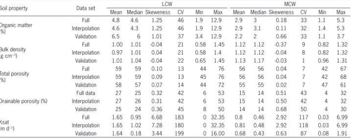
The descriptive statistics shown in Table 2 pres-ents the different variations of the physical properties. The interpolation and validation data sets were repre-sentative and appropriate because they have similar sta-tistical characteristics with the full data set. As a general trend, LCW has greater values of organic matter due the combination of type of native forest (rain forest) and colder climate (Santos et al., 2013), lower values of bulk density and greater values of total porosity, drainable po-rosity and Ksat.
The environmental conditions at MCW generated a lower organic matter content, because the carbon oxi-dizes more readily under warmer climates and lower rainfall, and due to the predominance of pasture in the area. It is well known that Oxisols have good physical properties with strong aggregate stability. However, this phenomenon is usually better expressed in the B hori-zon. Topsoil physical properties are more influenced by land use than other factors. MCW showed general trend of lower CV values, except for Ksat, whose values were the highest among the physical properties at both water-sheds. These findings are in agreement with MCW older and more highly weathered and stable soils.
Ordinary Kriging and Regression Kriging
Soil development, as well as soil properties, of-ten occur in response to the way in which water moves through and over the landscape, which is controlled by the local relief (Scull et al., 2003). Relief parameters control water and sediment distributions over the land-scape and terrain attributes that represent the dynam-ics of water movement are correlated with soil physical properties. These dependencies were detected by step-wise multiple linear regression models (Tables 3 and 4)
Table 2 − Descriptive statistics for soil physical-hydrological properties.
Soil property Data set LCW MCW
Mean Median Skeweness CV Min Max Mean Median Skeweness CV Min Max
Organic matter (%)
Full 4.8 4.6 1.25 46 1.9 12.9 2.9 3 0.18 33 1.1 5.3
Interpolation 4.6 4.3 1.25 46 1.9 12.9 2.9 3.1 0.11 32 1.4 5.3
Validation 6.5 6 1.01 37 3.4 12.9 2.2 2 0.66 33 1.1 3.7
Bulk density (g cm−3)
Full 1.00 1.01 -0.04 21 0.58 1.45 1.12 1.12 -0.37 9 0.82 1.32
Interpolation 0.97 1.01 0.04 21 0.58 1.4 1.12 1.12 -0.04 8 0.82 1.32 Validation 1.01 1.04 -0.04 22 0.65 1.45 1.13 1.17 -0.03 1 0.96 1.31
Total porosity (%)
Full 59 59 0.10 13 44 76 56 56 0.04 7 42 67
Interpolation 59 59 0.09 13 45 76 56 56 0.04 7 42 68
Validation 58 57 0.07 14 44 72 55 55 0.02 7 47 61
Drainable porosity (%)
Full data 27 25 0.32 42 6 53 15 14 0.51 43 4 32
Interpolation 27 26 0.31 42 6 53 15 14 0.50 42 4 32
Validation 25 24 0.36 45 8 50 14 14 0.68 50 4 30
Ksat (m d−1)
Full 1.65 0.95 6.68 183 0 32.35 0.8 0.46 2.92 117 0.03 6.99
Interpolation 1.65 1.02 7.28 180 0 32.35 0.81 0.48 2.92 118 0.03 6.99
Validation 1.64 0.18 3.44 199 0 16.00 0.68 0.43 0.63 87 0.08 1.91
and the Akaike criterion. The altitude and AACHN were some of the best predictors at the LCW and MCW ar-eas, respectively. These DTM parameters are related to different patterns of soil wetness, sediment movement (Schaetzl and Anderson, 2005), and land use, which in turn influence organic matter distribution.
Considering the factors of soil formation (Jenny, 1941), the NDVI was used to approximate the organism in terms of generalized land cover and land use (Malone et al., 2009). This index was shown to correlate well with the distribution of organic matter (Malone et al., 2009; Mendonça-Santos et al., 2010; Zhao and Shi, 2010), which in turn could influence soil physical properties. However, NDVI was only significantly correlated with organic matter at LCW.
The coefficient of determination (R2) is the propor-tion of variability of the interpolapropor-tion data set that is ac-counted by the statistical model. In comparison to MCW, R2 values at LCW are higher (from 0.15 to 0.30). Terrain analysis will be most useful in environments where the topographic shape is strongly related to the processes driving soil formation (McKenzie et al., 2000; Scull et al., 2003). The steep relief at LCW, with predominance of erosional surfaces, where mostly Inceptsols are formed and sediments have been deposited (Menezes et al., 2014), suggest some relationship, even low, between contemporaneous landforms and soil properties.
At MCW the predictors included in the model did not explain the variance of three physical properties, whose R2 values were less than 0.05. The hypothesis for the low or lack of correlation is related to complexity of relationships between environment and soil variables. These relationships may be complex, unknown, often very noisy, and not necessarely linear, as assumed by the multiple regression (Hengl et al., 2004; McKenzie and Ryan, 1999), and sometimes, only parts of the spa-tial structure can be described in a deterministic way
(Herbst et al., 2006). Also, other sources of variation re-lated to pedogenesis or land use might be responsible for the distribution of physical properties across the landscape. This study considered soil properties varying in lateral directions, and such variation can follow sys-tematic changes as a function of the landscape position, soil forming factors and/or soil management practices, where more studies are necessary.
The relationship between environmental and soil variables is not always linear and it is usually complex. Zhu et al. (2010) cited as an example of non-linearity and complexity the fact that a certain soil property might in-crease from a summit to backslope position and then de-crease from backslope to footslope or depressional posi-tions. Also, soil properties tend to change gradually within well-defined landscape units but change more quickly in transitional zones between landscape positions. Another point is that the main soil class at MCW are Oxisols. Such soils were formed in a ancient landscape, with distinct morphological features resulting from an environment of soil formation, which does not exist currently (Schaetl and Anderson, 2005). In other words, the contemporany landscape as well as topography or relief, were not pres-ent, when Oxisols were formed.
Neverthless, the multiple linear regression is one step of RK. A key issue is whether the correlations could be used to improve the prediction performance of soil properties.
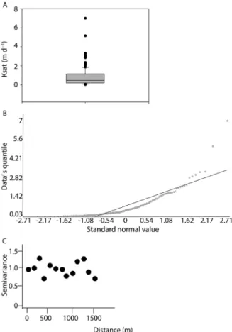
Highly variable soil properties make predictions more difficult and a decreased likelihood of attaining a reasonable estimate of the variogram (Armstrong, 1984). The Ksat showed outliers and a skewed distribution ac-cording to box plot graphics (Figure 3A and Figure 4A). The quantile values of the standard normal distribution are plotted on the x-axis in the Q-Q plot, and the cor-responding quantile values of the dataset are plotted on the y-axis. It is noticeable that points are deviating from
Table 3 − Stepwise multiple linear regression models between soil physical properties and environmental covariates at the Lavrinha Creek Watershed.
Soil Properties Intercept Altitude Slope WI Plan curvature Profile curvature NDVI R2 R2-adjusted
Organic matter (%) -10.91 0.0101 - - -0.115689 0.211202 4.734977 0.22 0.19
Bulk Density
(g cm−3) 2.26 -0.0010 0.00287 - - -0.0371671 - 0.20 0.17
Total porosity (%) 24.59 0.03702 -0.1629 -1.07596 0.48210 1.46226 - 0.19 0.16
Drainable porosity (%) -34.89 0.0501 -0.14237 - - - - 0.15 0.14
Ksat (m d−1) -5.50 0.0039 - - - - - 0.30 0.28
WI = wetness index; NDVI = normalized vegetation index.
Table 4 − Stepwise multiple linear regressions models between soil physical properties and environmental covariates at the Marcela Creek Watershed. Soil Properties Intercept AACHN Slope WI Plan curvature Profile curvature NDVI R2 R2-adjusted
Organic matter (%) 2.64 0.01249 - - - 0.05 0.03
Bulk Density (g cm−3) 1.299 -0.00107 - -0.0226413 - -0.0141589 - 0.12 0.08
Total porosity (%) 45.46 0.06602 - 0.95371 - 0.71823 - 0.12 0.08
Drainable porosity (%) 17.07 - -0.13880 - 0.89071 - - 0.05 0.03
Ksat (m d−1) 0.50 0.00633 - - - - - 0.04 0.03
the reference line (45˚), showing that Ksat has a non nor-mal distribution (Figure 3B and 4B).
Since the frequency distribution of Ksat is highly skewed and not normal, the data were log transformed, in agreement with the general thinking that the mea-surements of many natural phenomena tend to have a lognormal distribution (Moustafa, 2000). The variograms of the target data without transformation (Figures 3C and 4C) showed pure nugget effect. The transformation of the target data set was not necessary for the other soil physical attributes for OK analysis.
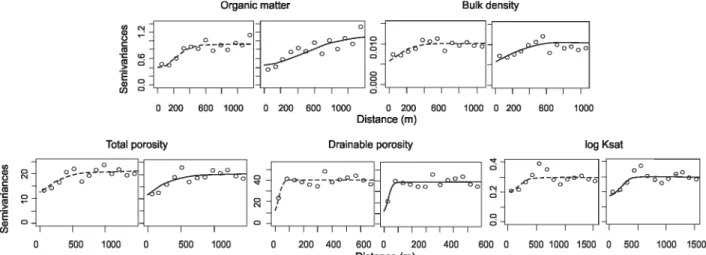
The parameters of variograms of targets (OK) and residuals of multiple linear regression are presented in Tables 5 and 6, and semivariograms presented in Figures 5 and 6. In general, the variograms of targets and residuals have approximately the same form and nugget, but the re-sidual variogram has a somewhat lower sill and range, in agreement with Hengl et al. (2007) and Hengl et al. (2004). Variograms have been used to describe and mea-sure the spatial structure of spatial data sets. A nugget to sill ratio (N/S) of 0.09 means that 9 % of the variabil-ity consists of unexplainable or random variation. Apart from random factors, structural factors, such as the par-ent material, terrain, and soil characteristics (e.g. tex-ture, mineralogy and pedogenic processes) can
co-deter-mine the soil properties. LCW showed stronger strength of spatial structure than MCW. And also, as long as the nugget effect is high, there may be undesirable large es-timates of variances, providing less smoother and less reliable OK maps (Moustafa, 2000). LCW showed higher CV and lower values of nugget/sill and nugget effect as well. The opposite situation occurred in the MCW, in disagreement with Utset et al. (2000).
Assessment of prediction methods
The comparison of prediction methods are shown in Table 7. The best prediction methods for each soil property presented the lowest MPE and RMSPE.
OK is known to be very sensitive to short-range variation (Laslett and McBratney, 1990), and the large RMSPE can be ascribed to this, especially at LCW. The values of MPE are lower in general. This method might be more appropriate when the complexity of pedogen-esis is too large to be captured in a deterministic way (Herbst et al., 2006). Utset et al. (2000) reported that soil properties were more precisely estimated for those whose CV was the least. In this work, MCW showed the lowest values of CV and the OK performed better than LCW (higher values of RMSPE), when comparing the same physical properties.
Figure 3 −Box plot (A), Q-Q plot (B), and the empirical variogram of Ksat non-transformed (C) at the Lavrinha Creek Watershed.
Table 5 –Variogram parameters of target variables and the residuals of multiple linear regression at the Lavrinha Creek Watershed.
Soil property Model Target Residuals Nugget/sill1 Strength of spatial
structure2 Range (m) Partial sill Nugget Range (m) Partial sill Nugget
Organic matter (%) Gaussian 763.98 5.86 0.51 763.98 3.36 1.27 0.09 Strong
Bulk Density (g cm−3) Exponential 623.63 0.06 0 374.19 0.029 0.012 0.00 Strong
Total porosity (%) Exponential 584.64 81.21 0 454.71 53.86 9.62 0.00 Strong
Drainable porosity (%) Gaussian 618.37 144.26 36.07 701.57 117.82 45.31 0.25 Medium
logKsat (m d−1) Exponential 436.5 0.33 0.15 218.27 0.24 0.15 0.45 Medium
1Calculated from the target data set; 2Values < 0.25 being strong, 0.25-0.75 being medium, and > 0.75 being weak (Cambardella et al., 1994).
Table 6 − Variogram parameters of target variables and the residuals of multiple linear regression at the Marcela Creek Watershed.
Soil property Model Target Residuals Nugget/sill1 Strength of spatial
structure2 Range (m) Partial sill Nugget Range (m) Partial sill Nugget
Organic matter (%) Gaussian 311.80 0.52 0.39 279.6 0.49 0.39 0.75 Weak
Bulk Density (g cm−3) Spherical 571.60 0.0044 0.0058 714.5 0.0038 0.0058 1.32 Weak
Total porosity (%) Exponential 817.00 14.06 12.14 545.68 11.22 11.22 0.86 Weak
Drainable porosity (%) Gaussian 36.38 29.50 11.78 36.38 28.10 11.78 0.39 Medium
logKsat (m d−1) Gaussian 332.60 0.11 0.20 291.04 0.09 0.21 1.82 Weak
1Calculated from the target data set; 2Values < 0.25 being strong, 0.25-0.75 being medium, and > 0.75 being weak (Cambardella et al., 1994).
Figure 5 − Variograms of target variables (dashed line) and the residuals of linear regression (right side) at the Lavrinha Creek Watershed.
RK takes into account the random component and the spatial structure of the target variables, derived from the spatial distribution of the auxiliary variable. So, the re-lationship between target soil property and auxiliary vari-ables, represented by their coefficient of determination, is important in determining if RK would outperform OK (Kravchenko and Robertson, 2007). Herbst et. al. (2006) found R2 from 0.20 to 0.55 in a correlation between soil hydraulic properties and terrain attributes, and RK out-performed OK on the topsoil. Zhu and Lin (2010) reported that RK outperform OK when R2 > 0.2 and the spatial structure was well captured by the training data set (ratio of sample spacing over correlation range). López-Granados et al. (2005) and Sumfleth and Duttman (2008) pointed out that even the incorporation of a rather weakly correlated co-variable – but significant - into RK tends to improve soil property prediction compared with OK. Zhao and Shi (2010) reported that only 19 % (R2 = 0.195) of a total varia-tion of organic carbon was explained by multiple linear regression between organic carbon and terrain attributes and NDVI attributes; and RK explained 65 %. Besides the coefficient of determination, some studies also pointed out the importance of the strength of spatial variability (nugget/sill). Kravchenko and Robertson (2007) and Zhu and Lin (2010) reported that RK did not outperform OK for soil properties with nugget/sill < 0.2 or R2 < 0.6.
In this study, if the predictive variables can explain even a small part of the variation in the target variable, RK outperforms OK because it exploits extra informa-tion. Furthermore, the summation of kriged errors due to regression, lead to smoothing of the predicted values, hence the reduction of RMSPE (Odeh et al., 1994). Ac-cording to Bishop and McBratney (2001), even when only poorly correlated secondary attributes are available, the hybrid methods may still perform better than OK. In this study, the RK outperformed OK when the strength of the relationship between soil properties and predic-tive variables is greater (R2 > 0.12) and/or with stronger strength of spatial structure, which was found in LCW for organic matter, bulk density and total porosity pre-diction. Greater values of CV were found at LCW, where the higher number of samples should be necessary to account for the spatial variability of physical properties.
MCW showed weak strength of spatial variability (N/S) and correlation between target and ancillary
vari-ables. With R2 of 0.12, the RK did not outperform the OK in the total porosity prediction, but did for bulk density. The prediction of organic matter, drainable porosity and Ksat by RK were not even performed, due the low coef-ficient of determination (R2 < 0.06), because it results in pure kriging (no correlation) (Hengl et al., 2007).
Considering the improvement over the OK, which is a geostatistical technique that considers only the spa-tial autocorrelation of observed values in field samples, the values of RI (%) showed that the prediction accuracy can be improved by incorporating ancillary variables into a prediction. However, RI should be analyzed along with the other statistical indexes of validation for a cor-rect analyzis of map reliability.
Predictive maps
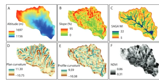
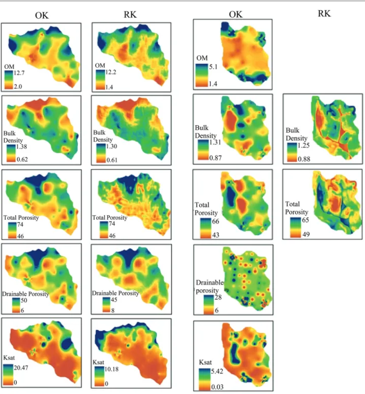
The DTMs and NDVI used for RK are presented in the Figures 7 and 8. The spatial prediction maps of OK and RK are presented in the Figures 9 and 10 for LCW and MCW, respectively.
The OK prediction maps show gradual transi-tions with fairly low level of detail. One limitation of this method, where the prediction has been based on an empirical model of soil variation, expressed in spatial terms, is the exclusion of information on soil-landscape relationships (McKenzie and Austin, 1993). Another is-sue was the bull-eyes features in the map of drainable porosity (LCW), as a result of a range dependence short-er than the distances to the nearest neighbours. The RK maps reflect changes of the DTMs and NDVI that were kept on multiple regression by the AIC criterion. And also, the RK, which uses auxiliary variables, has a smoothing effect on minimizing the influence of outliers on the prediction performance (Odeh et al., 1994). Such effect is valid only in cases for which R2 vaues are higher and there is no noise close to the random error.
At LCW, the spatial variability of physical and chemical properties are clearly influenced by land use in this watershed. The native forest of the Mantiquei-ra Range is restricted to hill areas and high elevations, which are inadequate for agriculture. The pattern of physical properties is quite similar to this pattern. The relief seems to influence the forest cover indirectly, since pasture is preferably implanted in flatter and lower ar-eas. Also, the greater organic matter content detected
Table 7 – Comparison of interpolation methods and relative improvement.
Soil property OK RK RI (%) OK RK RI (%)
MPE RMSPE MPE RMSPE MPE RMSPE MPE RMSPE
LCW MCW
Organic matter (%) -0.663 3.317 -0.482 2.408 27.4 0.146 0.659 - -
-Bulk density (g cm−3) 0.009 0.045 0.002 0.012 73.3 -0.005 0.063 -0.015 0.023 63.5
Total porosity (%) -0.312 1.562 -0.212 1.462 6.4 0.056 0.250 0.517 2.312
-Drainable porosity (%) -1.461 7.305 -1.460 7.301 0.1 0.936 4.188 - -
-Ksat (m d–1) 0.439 2.196 0.242 1.208 45.0 0.087 0.368 - -
Figure 8 − Digital terrain models (A, B, C, D, E) and normalized vegetation index - NDVI (F) at the Marcela Creek Watershed. Figure 7 − Digital terrain models (A, B, C, D, E) and normalized vegetation index - NDVI (F) at the Lavrinha Creek Wateshed.
at higher altitudes was probably due to lower temper-atures. Organic matter has been identified as a major controlling factor in aggregate stability (Angers et al., 1997). Vegetation distribution controls organic matter (Gessler et al., 2000), which in turn might explain the lower bulk density, higher total porosity, higher drain-able porosity and Ksat in the same portions of the land-scape, where land use is native forest. This spatial trend was accounted for the two prediction methods. At MCW, it is possible to see the influence of alluvium areas in the prediction of bulk density and total porosity, which was well captured by the WI (Figure 7C) and the profile cur-vature. The accumulation of organic matter in the flood-plains (low slopes and higher WI) was not accounted by OK. Water distribution in landscapes tightly controls soil carbon dynamics (Gessler et al., 2000), even though the floodplain did not show greater values of organic matter which may be due to the very high vertical and lateral spatial variability of characteristics, which is typical of these lowland environments.
Oxisols tend to have good physical properties in-fluenced by aggregate stability, as previously mentioned. Differently from the other physical properties, the Ksat values represent the topsoil depth, but this property is also influenced by soil properties at deeper depths. Al-though higher values of Ksat were expected in Oxisols, lower values of Ksat were found maybe due to cattle compaction in pastures, which is the main land use of this area, corroborating with increasing bulk density and decreasing total porosity and drainable porosity.
Conclusions
A better linear correlation between auxiliary variables and soil properties found at LCW, suggests some relationship between contemporaneous land-forms and soil properties, and RK outperformed OK .In most cases, RK were not performed at MCW due to lack of linear correlation between covariates and soil
Figure 9 − Ordinary kriging (OK) and regression kriging (RK) prediction maps of soil physical and chemical properties at the Lavrinha Creek Watershed. OM = organic matter; Ksat = saturated hydraulic conductivity.
Figure 10 − Ordinary kriging (OK) and regression kriging (RK) prediction maps of soil physical and chemical properties at the Marcela Creek Watershed. OM = organic matter; Ksat = saturated hydraulic conductivity.
Since landuse can affect surface properties espe-cially organic matter, a better understanding of the rela-tionship of landuse and soil carbon is required to provide better spatial predictions and estimates of soil carbon.
References
Angers, D.A.; Bolinder, M.A.A.; Carter, M.R.; Gregorich, E.G.; Simard, R.R.; Donald, R.G.; Beyaeart, R.P.; Martel, J. 1997. Impact of tillage practices on organic carbon and nitrogen storage in cool humid soils of eastern Canada. Soil and Tillage Research 41: 191-201.
Armstrong, M. 1984. Common problems seen in variograms. Mathematical Geology 16: 305-313.
Beskow, S.; Mello, C.R.; Norton, L.D.; Curi, N.; Viola, M.R.; Avanzi, J.C. 2009. Soil erosion prediction in the Grande River Basin, Brazil using distributed modeling. Catena 79: 49-59. Beven, K.; Wood, E.F. 1983. Catchment geomorphology and the
dynamics of runoff contributing areas. Journal of Hydrology 65: 139-158.
Bishop, T.F.A.; McBratney, A.B. 2001. A comparison of prediction methods for the creation of field-extent soil property maps. Geoderma 103: 149-160.
Cambardella, C.A.; Moorman, T.B.; Novak, J.M.; Parkin, T.B.; Karlen, D.L.; Turco, R.F. 1994. Field-scale variability of soil properties in Central Iowa soils. Soil Science Society of America Journal 58: 1501-1511.
Cressie, N. 1993. Statistics for Spatial Data. Wiley, New York, NY, USA.
Dobos, E.; Hengl, T. 2009. Soil mapping applications. p. 461-480. In: Hengl, T.; Reuter, H.I., eds. Developments in soil science. Elsevier, Amsterdam, Netherlands.
Draper, N.; Smith, H. 1998. Applied Regression Analysis. Wiley, New York, NY, USA.
Empresa Brasileira de Pesquisa Agropecuária. [EMBRAPA]. 1997. Manual of Soil Analysis Methods. = Manual de Métodos de Análises de Solo. Centro Nacional de Pesquisa de Solos, Rio de Janeiro, RJ, Brazil (in Portuguese).
Gessler, P.E.; Chadwick, O.A.; Chamran, F.; Althouse, L.; Holmes, K. 2000. Modeling soil-landscape and ecosystem properties using terrain attributes. Soil Science Society of America Journal 64: 2046-2056.
Goovaerts, P. 1999. Geostatistics in soil science: state-of-the-art and perspectives. Geoderma 89: 1-45.
Grunwald, S. 2009. Multi-criteria characterization of recent digital soil mapping and modeling approaches. Geoderma 152: 195-207.
Hengl, T.; Heuvelink, G.; Rossiter, D.G. 2007. About regression-kriging: from equations to case studies. Computer and Geosciences 33: 1301-1315.
Hengl, T.; Heuvelink, G.; Stein, A.A.A. 2004. Generic framework for spatial prediction of soil variables based on regression-kriging. Geoderma 122: 75-93.
Herbst, M.; Diekkrü, B.; Vereecken, H. 2006. Geostatistical co-regionalization of soil hydraulic properties in a micro-scale catchment using terrain attributes. Geoderma 132: 206-221. Jenny, H. 1941. Factors of Soil Formation. McGraw-Hill, New
York, NY, USA.
Kravchenko, A.N.; Robertson, G.P. 2007. Can topographical yield data substantially improve total soil carbon mapping by regression kriging? Agronomy Journal 99: 12-17.
Laslett, G.M.; McBratney, A.B. 1990. Further comparison of spatial methods for predicting soil pH. Soil Science Society of America Journal 54: 1533-1558.
López-Granados, F.; Jurado-Exposito, M.; Pena-Barragan, J.; Garcia-Torres, L. 2005. Using geostatistical and remote sensing approaches for mapping soil properties. European Journal of Agronomy 33: 279-289.
Malone, B.P.; Mcbratney, A.B.; Minasny, B.; Laslett, G.M. 2009. Mapping continuous depth functions of soil carbon storage and available water capacity. Geoderma 154: 138-152.
McBratney, A.; Odeh, I.; Bishop, T.; Dunbar, M.; Shatar, T. 2000. An overview of pedometric techniques for use in soil survey. Geoderma 97: 293-327.
McBratney, A.B.; Santos, M.L.M.; Minasny, B. 2003. On digital soil mapping. Geoderma 117: 3-52.
McKenzie, N.J.; Austin, M.P. 1993. A quantitative Australian approach to medium and small scale surveys based on soil stratigraphy and environmental correlation. Geoderma 57: 329-355.
McKenzie, N.J.; Gessler, P.E.; Ryan, P.J.; O’Connell, D. 2000. The role of terrain analysis in soil mapping. p. 245-265. In: Wilson, J.; Gallant, J., eds. Terrain analysis: principles and applications. John Wiley, New York, NY, USA.
McKenzie, N.J.; Ryan, P.J. 1999. Spatial prediction of soil properties using environmental correlations. Geoderma 89: 67-94. Mendonça-Santos, M.L.; Dart, R.O.; Santos, H.G.; Coelho, M.R.;
Berbara, R.L.L.; Lumbreras, J.F. 2010. Digital soil mapping of topsoil organic carbon content of Rio de Janeiro state, Brazil. p. 255-265. In: Boettinger, J.L.; Howell, D.W.; Moore, A.C.; Hartemink, A.E.; Kienast-Brown, S., eds. Digital soil mapping: bridging research, environmental application, and operation. Springer, Dordrecht, Netherlands.
Menezes, M.D.; Silva, S.H.G.; Mello, C.R.; Owens, P.R.; Curi, N. 2014. Solum depth spatial prediction comparing conventional with knowledge-based digital soil mapping approaches. Scientia Agricola 71: 316-323.
Mora-Vallejo, A.; Claessens, L.; Stoorvogel, J.; Heuvelink, G.B.M. 2008. Small scale digital soil mapping in Southeastern Kenya. Catena 76: 44–53.
Moustafa, M.M. 2000. A geostatistical approach to optimize the determination of saturated hydraulic conductivity for large-scale subsurface drainage design in Egypt. Agricultural Water Management 42: 291-312.
Odeh, I.O.A.; Mcbratney, A.B.; Chittleborough, D. 1995. Further results on prediction of soil properties from terrain attributes: heterotopic cokriging and regression-kriging. Geoderma 67: 215-226.
Odeh, I.O.A.; Mcbratney, A.B.; Chittleborough, D. 1994. Spatial prediction of soil properties from landform attributes derived from a digital elevation model. Geoderma 63: 197-214. Rykiel, E. 1996. Testing ecological models: the meaning of
validation. Ecological Modeling 90: 229-244.
Schaetzl, R.; Anderson, S. 2005. Soils: Genesis and Geomorphology. Cambridge University, Cambridge, England.
Scull, P.; Franklin, J.; Chadwick, O.A.; McArthur, D. 2003. Predictive soil mapping: a review. Progress in Physical Geography 27: 171-197.
Silva, S.H.G.; Owens, P.R.; Menezes, M.D.; Santos, W.J.R.; Curi, N. 2014. A technique for low cost soil mapping and validation using expert knowledge on a watershed in minas gerais, Brazil. Soil Science Society of America Journal 78: 1310-1319. Sumfleth, K.; Duttmann, R. 2008. Prediction of soil property
distribution in paddy soil landscape using terrain data and satellite information as indicators. Ecological Indicators 8: 485-501.
Utset, A.; López, T.; Díaz, M. 2000. A comparison of soil maps, kriging and a combined method for spatially predicting bulk density and field capacity of ferralsols in the Havana-Matanzas Plain. Geoderma 96: 199-213.
Walkley, A.; Black, I.A. 1934. An examination of the Degtjareff method for determining soil organic matter and a proposed modification of the chromic acid titration method. Soil Science 37: 29-38.
Webster, R.; Oliver, M.A. 2007. Geostatistics for Environmental Scientists. John Wiley, New York, NY, USA.
Zhao, Y.C.; Shi, X.Z. 2010. Spatial prediction and uncertainty assessment of soil organic carbon in Hebei Province, China. p. 227-239. In: Boettinger, J.L.; Howell, D.W.; Moore, A.C.; Hartemink, A.E.; Kienast-Brown, S., eds. Digital soil mapping: bridging research, environmental application, and operation. Springer, Dordrecht, Netherlands.
Zhu, Q.; Lin, H.S. 2010. Comparing ordinary kriging and regression kriging for soil properties in contrasting landscapes. Pedosphere 20: 594-606.