GENETIC PARAMETERS FOR POST WEANING GROWTH
OF NELLORE CATTLE USING POLINOMYALS AND
TRIGONOMETRIC FUNCTIONS IN RANDOM
REGRESSION MODELS
Osmar Jesus Macedo1,2; Décio Barbin3*; Gerson Barreto Mourão3
1
UFMS - Depto. de Ciências Exatas, Campus Três Lagoas, C.P. 210 - 79620-080 - Três Lagoas, MS - Brasil.
2
USP/ESALQ - Programa de Pós-Graduação em Estatística e Experimentação Agronômica.
3
USP/ESALQ - Depto. de Ciências Exatas, C.P. 9 - 13418-900 - Piracicaba, SP - Brasil. *Corresponding author <[email protected]>
ABSTRACT: Covariance functions and random regression models have been considered as an alternative for data adjustment, in sequence, stemming from the same animal along time and which presents a structured pattern of covariance. Aiming to evaluate the performance of random regression models based on the Legendre, modified Jacobi and trigonometric functions, data concerning the weights of Nellore breed animals were used from birth to the 800th day of life, in models that assumed
direct additive and animal permanent environmental effects coefficients. The Schwarz Bayesian information criterion (BIC) led to the selection of the models Legendre of order six (ML6), Jacobi of order five (MJ5) and trigonometric of order six (MT6), the ML6 model presenting the lowest BIC. At the extremity of the interval, the MJ5 model presented lower variance of component estimates than those obtained through the ML6 model, however the estimates were in accordance to the medium part of the interval; while the estimates from the MT6 model were oscillating and different from those obtained through the other models. At the extremity of the interval, the heritability coefficient estimates ( ) obtained through the MJ5 model were lower than those obtained through the ML6 model, however, in the medium part of the interval, they were in accordance, remaining between 0.2 and 0.3. The values obtained through the MT6 model were different from those obtained through the other models, remaining between 0.35 and 0.40 on the first 285th days and then dropping to 0.01 on the 800th days of
life. The means of the estimated growth curves started to distance from the data mean tendency from the 470th days on, and in this interval, the MT6 model was the most suitable.
Key words: additive variance, heritability, Jacobi, Legendre, longitudinal data
PARÂMETROS GENÉTICOS PARA CRESCIMENTO PÓS-DESMAME
DE BOVINOS NELORE POR MEIO DE FUNÇÕES POLINOMIAIS E
TRIGONOMÉTRICAS EM MODELOS DE REGRESSÃO ALEATÓRIA
RESUMO: O uso de funções de covariância e regressão aleatória tem sido considerado como uma alternativa para o ajuste de dados longitudinais com estrutura de covariância padrão, pois são mensurados no mesmo animal ao longo do tempo. Com objetivo de avaliar o desempenho dos modelos de regressão aleatória nas bases de funções de Legendre, de Jacobi modificada e as trigonométricas, os dados referentes aos pesos de animais da raça Nelore do nascimento aos 800 dias foram analisados com modelos que assumiram coeficientes de efeito aditivo direto e de ambiente permanente de animal. O critério de informação Bayesiano de Schwarz (BIC) conduziu a seleção dos modelos Legendre de ordem seis (ML6), Jacobi de ordem cinco (MJ5) e trigonométrica de ordem seis (MT6), dos quais, ML6 foi o modelo com o menor BIC. O modelo MJ5 apresentou estimativas de componentes de variância abaixo das estimativas obtidas pelo modelo ML6 nos extremos do intervalo e estimativas muito próximas no seu interior. Já as estimativas do modelo MT6 foram oscilantes e distintas das estimativas obtidas pelos demais modelos. Os coeficientes de herdabilidade ( ) estimados pelo modelo MJ5 ficaram abaixo das estimativas do modelo ML6 nos extremos do intervalo e no seu interior foram concordantes, entre 0,2 e 0,3. As estimativas obtidas pelo modelo MT6 se diferenciaram dos demais modelos, variando entre 0,35 e 0,40 aos 285 dias e diminuindo para 0,01 aos 800 dias de idade. As médias das curvas de crescimento estimadas se afastaram da tendência média dos dados a partir da idade 470 dias, e nesse intervalo a curva que mais se aproximou foi obtida pelo modelo MT6.
INTRODUCTION
Covariance functions and random regression mod-els have been considered as an alternative for the ad-justment of data obtained in sequence from the same animal along time and which presents a structured pat-tern of covariance. This occurs due to the fact that phenotypic characteristics can be measured using same animal for a large number of times. Considering these unique characteristics, the results can be modeled us-ing a continuous function based on the Legendre poly-nomials, especially after Kirkpatrick et al. (1990).
Polynomial regressions of 4th and 5th degrees
pre-sented better results for estimating genetic additive and maternal permanent environment effects using random regression to analyze data concerning growth measures of the Guzerath breed cattle (Scarpel, 2004). In addi-tion, these polynomials present problems, producing variance components and genetic parameter estimates, at the interval extremities, which may not be reliable (Meyer, 2005). Those problems are due to the strong oscillation that the Legendre polynomials present at the extremities of the interval [-1, 1].
Considering these problems, this study aims to identify possible differences in the random regression model adjustments when they are influenced by the Legendre polynomials, modified Jacobi and trigonomet-ric functions, considering their application in data mod-eling related to body weight measures of the Nellore breed. The objectives were to compare fitted groyth curves of animal weight post weaning; to investigate the behavior of the estimated random components of the curves; and to exam the behavior of the heritabil-ity coefficients of the curves.
MATERIAL AND METHODS
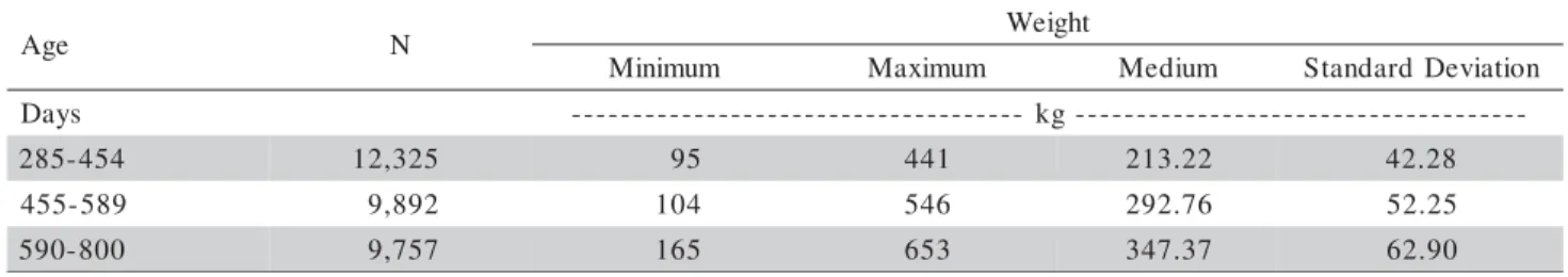
Data files consisted of 61,975 body weights mea-sured on 20,543 animals which were kept grazing on tropical pastures, in Uberaba, Minas Gerais State, Brazil (19o45’ S; 47o55’ W), and in addition information from
26,275 pedigree Nellore animals was included. No mal was weighed more than six times, and each ani-mal supplied at most, one measure within each of the following age intervals (in days): 1-69, 70-159,
160-284, 285-454, 455-589 and 590-800 (brief description of the data is shown in Table 1). Weighing was per-formed between 1981 and 2002.
Data were organized in 670 contemporaneous groups (GC), considering the management group, the weaning (205 days), the year of birth and sex in each interval. Each GC consisted of weights of at least 18 animals, belonging to the offsprings of at least two dif-ferent bulls. In addition, the data were classified into seven classes, named CIMP, according to the ages of dams at calving.
The purpose of this study was to consider random regression models that assume additive genetic and animal permanent environment effect coefficients as random factors. Therefore, all the data analysis was done using random regression models in which the or-thonormal functions of the animal ages were consid-ered as covariables of the random coefficients. Be-sides, a cubic regression using the Legendre polyno-mials (without the Legendre polynomial of degree zero) was added to the fixed effects of the model.
Data were disposed into six intervals, so that there were six random factors of possible maximum order of adjustment. The expressions of the functions be-longing to the bases applied to this study were obtained through the Gram-Schmidt process of sequences of orthonormalization functions. A space coordinate X of all the functions within the domain [-1, 1] and having the internal product (Kreyszig, 1978) given by <x, y>
= x(t) y(t)dt, x, y ∈ X, defines a Hilbert space, which is represented by L2 [-1, 1].
Take the power functions, ϕ0(t) = 0, ϕ1(t) = t, ϕ2(t)
= t2, ..., ϕj(t) = tj,
t ∈ [–1, 1]; take Δ(t) = (a + bt)α (a
– bt)β, being α > –1, β > –1; a, b∈ R and a≠b if a
= 0 or b = 0; the restrictions on α and β are needed
to justify the integrability of Δ in the [-1, 1] interval; if α and β assume positive integer values, Δ is a poly-nomial function and, therefore, x0, x1, x2, ..., in which
x0(t) = ϕ0(t)Δ(t), x1 = ϕ1(t)Δ(t), x2 = ϕ2(t)Δ(t), ..., xj=
ϕj(t)Δ(t), t ∈ [–1, 1] is a sequence of polynomials of
weight Δ; then, in order to orthonormalize the (xi)i∈N sequence, the Gram-smith process is once more used, considering the internal product defined in the L2 [–1,
1] space. If α = β = 0 in Δ(t), the result is a constant
weight function, therefore, {x0, x1, ..., xj, becomes a
e g
A N Weight
m u m i n i
M Maximum Medium StandardDeviation
s y a
D --- kg---
-4 5 4 -5 8
2 12,325 95 441 213.22 42.28
9 8 5 -5 5
4 9,892 104 546 292.76 52.25
0 0 8 -0 9
5 9,757 165 653 347.37 62.90
sequence of power functions and its orthonormalization produces a base for the Legendre polynomial functions.
The base of modified Jacobi polynomial functions, (ϖn)n∈N , can be obtained through the use of the Gram-Schimidt process in the orthonormalization of the se-quence (xn)n∈N = (ϕnΔ)n∈N being, Δ(t) = (1 – 1/2t).
The sequence {1, cos(t), sin(t), cos(2t), sin(2t),
...,cos(kt), sin(kt) orthonormalized by the
Gram-Schmidt process, with the internal product given by <x, y> = x(t) y(t)dt, x, y∈ X, generates the base of the trigonometric functions with the domain [0, 2π]. The following random regression model (Kirkpatrick et al., 1990; Meyer, 1998) was used:
in which, yij is the ith animal weight at its jth age; F
represents part of the fixed effects; is the jth age for the ith animal, standardized for the domain interval
as-sociated to the base of the orthonormal functions used in the adjustment; φm ( ) is the m
th Legendre
polyno-mial evaluated in ; βm is the mth regression coefficient
of the fixed effect of the weight at the age; αim and
γim are the mth random regression coefficients for the
direct additive genetic and permanent environment ef-fects, respectively, for the ith animal; ψm ( ) represents
a function of the Legendre or Modified Jacobi or-thonormal base or of the trigonometric functions evalu-ated in ; ka = kp ∈ {2, 3, 4, 5, 6} is the order of adjustment of the orthonormal functions and εij is the
random error.
The F term of the model includes the fixed effects of GC and CIMP. The random regression model in its matrix form is:
y = Xb + Z* a + Z*Dp + ε,
in which, y = [y1, y2, ..., y20.543] is the vector
corre-sponding to the weight of the 20,543 animals. The weight of individuals was disposed, always, after the weight of their ancestors and in crescent or-der of age at the time of the weighing. The incidence matrix for the models fixed effects is represented by
X, b is the fixed effect parameter vector given by b =
[CIMP1, CIMP2, ..., CIMP7, GC1, GC2, ..., GC670, β1, β2, β3].
The vectors a = [a1, a2, ..., a20.543] and [p1, p2, ..., p20.543] represent the random regression models for
ad-ditive genetic and animal permanent environmental ef-fects, respectively, and ε is the residual vector.
The matrixes Z* and are the incidence matrixes
of the random factors and their elements are null, they are the images of functions that belong to one of the bases of the orthonormal functions.
If KA = cov(a, a) and Kp= cov(p, p), then KA and Kp are called coefficient matrixes for the additive ge-netic and animal permanent environment covariance functions, G0 and C0, respectively.
It was assumed that the fixed part of the model takes into account the systematic effects of age, which means that a ~ N(0, KA ⊗A) and p ~ N(0, KP ⊗I20.543), and that cov(a, p) = 0. It was also assumed that V
(ε) = R, which means that the expression of the
re-stricted likelihood function logarithm for the random regression model (Meyer, 1989, 1998) is given by:
– 2L(θ) = const + NA ln(⏐KA⏐) + Ka ln(⏐A⏐) + ND
ln(⏐KP⏐) + ln(⏐R⏐) + ln(⏐C*⏐) + yTPy,
in which, θ is the vector formed by the parameters that are presented as the matrixes KA and KP elements, NA is the total number of animals in the analysis, ND is
the number of animals that provided the data, A is the kinship matrix, C* is the mixed model equations co-efficients matrix and P = V–1 – V–1 X(XTV–1X) XTV–1,
being Var(y) = V
The WOMBAT device (Meyer, 2006) was used for the data analysis. Among the many available algorithms of this device, the PX-AI algorithm was chosen, be-cause, it combines the PX (parameter expanded) method, which is a variation of the EM (expectation-maximization) algorithm, with the AI (average infor-mation) algorithm (Meyer, 1997).
The assessment of the best fitted model is given in relation to the maximum likelihood ratio test (LRT), the Akaike information criterion (AIC) and the Schwarz Bayesian criterion (BIC). The AIC and BIC criteria ap-ply penalties for the number of estimated parameters.
For each base of orthonormal functions, Legendre, modified Jacobi and trigonometric, five random regres-sion models were analyzed, assuming heterogeneity of the residual variances in the six age sub-intervals.
To simplify the presentation of the results, the ran-dom regression models were identified through MBm, in which, M stands for model, B stands for the base of orthonormal functions used in the analysis, which can be L = Legendre, J = Jacobi and T = Trigono-metric; m ∈ {2, 3, 4, 5, 6} represents the adjustment order of the random coefficients assumed by the model.
RESULTS AND DISCUSSION
There were differences, according to the LRT (Table 2), between the likelihood function logarithm values χ2
12 in the three bases of orthonormal functions,
suitable situation for the data in each of the base of or-thonormal functions occurred in the models with 48 parameters. The ML6 and MT6 models were selected according to the AIC and BIC criteria. For the base of modified Jacobi functions, the AIC criterion, led to the selection of the MJ6 model, however the BIC criterion led to the selection of the MJ5 model. In this case, con-sidering the parsimony, because of the lowest number of estimated parameters, the MJ5 model was chosen.
Among the ML6, MJ5 and MT6 models, the log val-ues (L) and the AIC and BIC criteria indicated that the ML6 model was the one that was best adjusted to the data.
The direct additive genetic variance curves (Fig-ure 1) presented a very strong growth tendency up to the 600 days, reaching their peak and then plunging in the last subinterval of the age domain. The curves estimated through the ML6 and MJ5 models became more appart from each other at the beginning and end of the age interval and the curve estimated through the MT6 model presented a particularly strong oscillation as compared to the other curves. Probably the pres-ence of data concerning animals at ages higher than 650 days in the ML6 and MJ6 models could have in-fluenced the variance component estimates, and as a consequence, the h2 estimates.
l e d o
M 1 p L LRT AIC BIC
e r d n e g e L 2 L M ) 1
( 12 -203,529.762 - 407,083.524 407,191.806
3 L M ) 2
( 18 -201,796.064 (2 - 1) 1,733.698 403,628.128 403,790.552
4 L M ) 3
( 26 -200,923.027 (3- 2) 873.037 401,898.054 402,132.664
5 L M ) 4
( 36 -200,730.423 (4 - 3) 192.604 401,532.846 401,857.690
6 L M ) 5
( 48 -200,618.053 (5 - 4) 112.370 401,332.106 401,765.232
i b o c a J d e i f i d o M 2 J M ) 1
( 12 -202,771.126 - 405,566.252 405,674.534
3 J M ) 2
( 18 -201,970.384 (2 - 1) 800.742 403,976.768 404,139.190
4 J M ) 3
( 26 -200,983.466 (3- 2) 986.918 402,018.932 402,253.542
5 J M ) 4
( 36 -200,700.086 (4 - 3) 283.380 401,472.172 401,797.018
6 J M ) 5
( 48 -200,654.785 (5- 4) 45.301 401,405.570 401,838.698
c i r t e m o n o g i r T 2 T M ) 1
( 12 -206,616.633 - 413,257.266 413,365.548
3 T M ) 2
( 18 -205,649.850 (2 - 1) 966.783 411,335.700 411,498.122
4 T M ) 3
( 26 -202,973.719 (3- 2) 2,676.131 405,999.438 406,234.050
5 T M ) 4
( 36 -202,768.186 (4 - 3) 205.533 405,608.372 405,933.218
6 T M ) 5
( 48 -201,806.617 (5 - 4) 961.569 403,709.234 404,142.360
Table 2 - Number of parameters (p), value of the likelihood function logarithm (L), likelihood ratio test (LRT), Akaike information criterion (AIC) and Schwartz Bayesian information criterion (BIC) for the fitted random regression models with different orders for the additive genetic and animal permanent environment effects.
1ML6 = model fitted through Legendre functions of order six; MJ6= model fitted through modified Jacobi functions of order six; MT6
= model fitted through trigonometric function of order six
The animal permanent environment variance curves (Figure 2) reached the peak between the sec-ond from last (454 – 589) and last (589 – 800) sub-intervals of the age domain and had then a strong de-crease near the top extremity of this interval, which indicates that the environmental effect prevailed over the additive genetic effect. The curves estimated through the ML6 and MJ5 models were distant from each other only at the end of the age interval. The curve estimated through the MT6 model presented strong oscillations being, once more, different from the other curves.
As a hypothesis, the variances of the residuals were considered as constant in each subinterval, which ex-plains the discontinuity (Figure 3). Accordingly, it can be verified that the curves estimated through ML6 and MJ5 were very close to each other, while the curve estimated through the MT6 model was different from the other curves, mainly in the second and sixth sub-intervals of the age domain.
Figure 1 - Direct additive genetic variance curves estimated by the Legendre order six (ML6), modified Jacobi order five (MJ5) and trigonometric order six (MT6) models.
Figure 3 - Residual variance curves estimated by the Legendre order six (ML6), modified Jacobi order five (MJ5) and trigonometric order six (MT6) models.
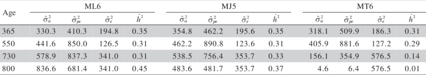
Table 3 - Variance components and heritability coefficients estimates for different ages obtained through the Legendre order six (ML6), modified Jacobi order five (MJ5) and trigonometric order six (MT6) models.
= additive direct genetic variance; = animal permanent environment effect variance; = residual variance; = heritability for direct effect;
e g
A ML6 MJ5 MT6
5 6
3 330.3 410.3 194.8 0.35 354.8 462.2 195.6 0.35 318.1 509.9 186.3 0.31
0 5
5 441.6 850.0 126.5 0.31 462.2 890.8 123.6 0.31 405.9 881.6 127.2 0.29
0 3
7 578.9 837.3 341.0 0.31 538.5 756.4 353.7 0.33 156.1 354.9 576.5 0.14
0 0
8 836.6 681.4 341.0 0.45 483.6 481.7 353.7 0.37 4.6 6.4 576.5 0.01
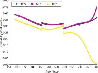
at the ages 365, 550 and 730 days, and presented huge differences at birth and at 800 days, the values esti-mated through the MJ5 model being smaller, which indicates that the random regression model under the influence of the modified Jacobi functions produces smoother curves at the extremities of the age inter-val (Figure 4), and that the random regression model
theory can contribute to solving problems associated to models that use the Legendre polynomials (Meyer, 2005).
For the values estimated through the MT6 model an oscillatory tendency was again verified, and that also the estimates for the ages 730 and 800 days were very low when compared to the heritability coefficients estimated through the ML6 and MJ5 models.
The models under the influence of these bases, the Legendre and modified Jacobi functions, presented similar results in the center of the domain, when com-pared to the variability of the Legendre functions at the extremities.
A univariate model for data composed of Nellore cattle weights (Figueiredo, 2001), obtained at the same farm, presented 0.29 as the h2 estimate at the
yearling stage. These values are not too distant from the heritability estimates obtained by the ML6 and MJ5 models at the yearling stage. Most recently, also with the same herd used in this study (Figueiredo et al., 2005), the h2 estimates were 0.34 and 0.36 for the weight traits at the yearling stage and at 18 months, respectively. At yearling, the estimate was very close to the ones obtained through the ML6 and MJ5 mod-els.
Figure 2 - Animal permanent environment variance curves estimated by the Legendre order six (ML6), modified Jacobi order five (MJ5) and trigonometric order six (MT6) models.
Additive
genetic
variance
(kg
)
2
250 300 350 400 450 500 550 600 650 700 750 800
Age (days) 0
100 200 300 400 500 600 700 800
MJ5 ML6 MT6
250 300 350 400 450 500 550 600 650 700 750 800
Age (days)
Animal
permanent
environment
al
varance
(kg
)
2
0 200 400 600 800 1000 1200 1400
MJ5 ML6 MT6
Residual
variance
(kg
)
2
0 100 200 300 400 500 600 700
250 300 350 400 450 500 550 600 650 700 750 800
Age (days)
Also an univariate analysis to study data collected from Nellore cattle (Oliveira, 2005), with a model con-sidered as direct additive genetic, direct maternal ge-netic and maternal permanent environment effects, re-sulted in h2 estimates as follows: 0.36; for the weight
at yearling, which was in accordance to the h2 values
estimated through the ML6 and MJ5 models at the yearling stage and at 18 months.
Also working with random regression models with classes of four days in the analysis of Nellore cattle weight, from birth to 630 days, Albuquerque & Meyer (2001) obtained h2 estimates between 0.2 and 0.4 from birth to 450 days, which were in disagreement with the h2 values estimated through the models of this
study, which showed h2 values higher than0.40 from birth to 284 days, probably due to the absence of the
maternal effect in the models. In addition, Albuquer-que & Meyer (2001) and Santoro et al. (2005), ob-tained h2 estimates between 0.4 and 0.6 for the inter-val of age ranging from 450 to 630 days, in disaggreement to the h2 values estimated by this study,
as well.
The ML6, MJ5 and MT6 allowed the estimation of the growth curve for each of the animals involved in the analysis. The graphic representation of all the growth curves estimated through the ML6, MJ5 and MT6 models is not easy to interpret, for this reason the curves obtained through all the growth curves fit-ted through each model are presenfit-ted in Figure 5, to-gether with the data means in each point in the inter-val [285, 800].
Finally, the absence of the maternal effect in the model should be considered. This may promote changes in the estimates, mainly up to the yearling stage; however, it should not jeopardize the analysis to express the methodological differences.
CONCLUSIONS
The differences in the variance curves constitute evidence to the nature of the functions belonging to the bases of the orthonormal functions, indicating that these different bases have influence on the variance component estimation, and as a consequence, influ-ence on the genetic parameter estimation.
The Legendre and modified Jacobi functions were of polynomial nature, but they show differences at the extremities due to the smaller variability of the modi-fied Jacobi functions at the beginning and end of the domain interval.
The trigonometric functions presented oscillatory variance curves through all their domain, which is un-desirable.
ACKNOWLEDGEMENTS
To CNPq and CAPES, for finantial support. To the Mundo Novo Farm (Uberaba, Minas Gerais, Brazil) and Grupo de Melhoramento Animal “Gordon Dickerson” from the Faculdade de Zootecnia e Engenharia de Alimentos of the University of São Paulo, for supplying the data.
REFERENCES
ALBUQUERQUE, L.G.; MEYER, K. Estimates of covariance functions for growth from birth to 630 days of age in Nellore cattle. Journal of Animal Science, v.79, p.2776-2789, 2001. FIGUEIREDO, L.G.G. Estimativas de parâmetros genéticos de características de carcaças feitas por ultra-sonografia em bovinos da raça Nelore. Pirassununga: USP/FZEA, 2001. 67p. Dissertação (Mestrado).
Figure 4 - Heritability coefficient curves at different ages estimated by the Legendre order six (ML6), modified Jacobi order five (MJ5) and trigonometric order six (MT6) models.
250 300 350 400 450 500 550 600 650 700 750 800
Age (days)
Herit
ability
coef
ficient
s
0.00 0.15 0.20 0.30 0.35 0.45 0.50
0.40
0.25
0.10
0.05
MJ5 ML6 MT6
Figure 5 - Means of the weight curves estimated by the Legendre order six (ML6), modified Jacobi order five (MJ5) and trigonometric order six (MT6) models, in relation to the average tendency of the data at each point of the age interval.
250 300 350 400 450 500 550 600 650 700 750 800
Age (days)
W
eight
(kg)
50 100 200 250 350 400 450
300
150
0
MJ5
ML6 MT6
FIGUEIREDO, L.G.G.; ELER, J.P.; MOURÃO, G.B.; FERRAZ, J.B.S.; BALIEIRO, J. C.C.; MATTOS, E.C. Análise genética do temperamento em uma população da raça Nellore. Livestock Research for Rural Development, v.17, 2005. Available at http://www.cipav.org.co/lrrd/lrrd17/ 7/gira17084.htm. Accessed 10 Aug. 2007.
KIRKPATRICK, M.; LOFSVOLD, D.; BULMER M. Analysis of the inheritance, selection and evolution of growth trajectories. Genetics, v.124, p.979-993, 1990.
KREYSZIG, E. Introductory functional analysis with applications. New York: John Whiley, 1978. 688 p. MEYER, K. WOMBAT: a program for mixed model analyses by
restricted maximum likelihood: user notes. Armidale: Animal Genetics and Breeding Unit, 2006. 55 p. Available in http:// agbu.une.edu.au~kmeyer/wombat.html. Accessed in 28 Mar. 2007.
MEYER, K. Random regression analyses using B-splines to model growth of Australian Angus Cattle. Genetics Selection Evolution, v.37, p.473-500, 2005.
MEYER, K. Estimating covariance functions for longitudinal data using a random regression model. Genetics Selection Evolution, v.30, p.221-240, 1998.
MEYER, K. An “average Information” restricted maximum likelihood algorithm for estimating reduced rank genetic covariance matrices or covariance functions for animal models with equal design matrices. Genetics Selection Evolution, v.23, p. 67-83, 1997.
Received September 10, 2007 Accepted December 12, 2008
MEYER, K. Restricted maximum likelihood to estimate variance components for animal models with several random effects using a derivative-free algorithm. Genetics Selection Evolution, v.21, p.317-340, 1989.
OLIVEIRA, H.P.Q. Análise genética dos efeitos de linhagem materna em um rebanho Nelore. Pirassununga: USP/FZEA, 2005. 91p. Dissertação (Mestrado).
SANTORO, K.R.; BARBOSA, S.B.P.; SANTOS, E.S.; BRASIL, H.A. Uso de funções de covariância na descrição do crescimento de bovinos Nelore criados no estado de Pernambuco. Revista Brasileira de Zootecnia, v.34, p.2290-2297, 2005. SCARPEL, L.C.P. Estimativas de parâmetros e valores