www.the-cryosphere.net/9/1505/2015/ doi:10.5194/tc-9-1505-2015
© Author(s) 2015. CC Attribution 3.0 License.
Impact of model developments on present and future simulations
of permafrost in a global land-surface model
S. E. Chadburn1, E. J. Burke2, R. L. H. Essery3, J. Boike4, M. Langer4,5, M. Heikenfeld4,6, P. M. Cox1, and P. Friedlingstein1
1Earth System Sciences, Laver Building, University of Exeter, North Park Road, Exeter EX4 4QE, UK 2Met Office Hadley Centre, Fitzroy Road, Exeter EX1 3PB, UK
3Grant Institute, The King’s Buildings, James Hutton Road, Edinburgh EH9 3FE, UK
4Alfred Wegener Institute, Helmholtz Center for Polar and Marine Research (AWI), 14473 Potsdam, Germany
5Laboratoire de Glaciologie et Géophysique de l’Environnement (LGGE), BP 96, 38402 St Martin d’Hères CEDEX, France 6Atmospheric, Oceanic and Planetary Physics, Department of Physics, University of Oxford, Parks Road,
Oxford OX1 3PU, UK
Correspondence to:S. E. Chadburn ([email protected])
Received: 25 February 2015 – Published in The Cryosphere Discuss.: 25 March 2015 Revised: 3 July 2015 – Accepted: 7 July 2015 – Published: 7 August 2015
Abstract.There is a large amount of organic carbon stored in permafrost in the northern high latitudes, which may become vulnerable to microbial decomposition under future climate warming. In order to estimate this potential carbon–climate feedback it is necessary to correctly simulate the physical dynamics of permafrost within global Earth system models (ESMs) and to determine the rate at which it will thaw.
Additional new processes within JULES, the land-surface scheme of the UK ESM (UKESM), include a representa-tion of organic soils, moss and bedrock and a modificarepresenta-tion to the snow scheme; the sensitivity of permafrost to these new developments is investigated in this study. The impact of a higher vertical soil resolution and deeper soil column is also considered.
Evaluation against a large group of sites shows the annual cycle of soil temperatures is approximately 25 % too large in the standard JULES version, but this error is corrected by the model improvements, in particular by deeper soil, organic soils, moss and the modified snow scheme. A comparison with active layer monitoring sites shows that the active layer is on average just over 1 m too deep in the standard model version, and this bias is reduced by 70 cm in the improved version. Increasing the soil vertical resolution allows the full range of active layer depths to be simulated; by contrast, with a poorly resolved soil at least 50 % of the permafrost area has a maximum thaw depth at the centre of the bottom soil
layer. Thus all the model modifications are seen to improve the permafrost simulations.
Historical permafrost area corresponds fairly well to ob-servations in all simulations, covering an area between 14 and 19 million km2. Simulations under two future climate scenarios show a reduced sensitivity of permafrost degra-dation to temperature, with the near-surface permafrost loss per degree of warming reduced from 1.5 million km2◦C−1
in the standard version of JULES to between 1.1 and 1.2 million km2◦C−1 in the new model version. However,
the near-surface permafrost area is still projected to approxi-mately half by the end of the 21st century under the RCP8.5 scenario.
1 Introduction
1.35◦C decade−1is observed in recent years, with large
po-tential impacts (Bekryaev et al., 2010; Stocker et al., 2013). Permafrost is of interest not only because of the physi-cal effects of permafrost thaw, but because it contains large quantities of stored organic carbon, approximately 1300– 1370 Pg (Hugelius et al., 2014), which may be released to the atmosphere in a warming climate. This could have a sig-nificant climate feedback effect, which needs to be included in global Earth system models (ESMs) in order to account for the full carbon budget in the future (Koven et al., 2011; MacDougall et al., 2012; Burke et al., 2012; Schneider von Deimling et al., 2012, 2014).
In order to simulate permafrost carbon feedbacks, the land-surface components of ESMs should include both an appropriate carbon cycle and a representation of the physi-cal dynamics. The amount of carbon released from the soil is strongly dependent on the physical state of the ground – the temperature of the permafrost and the rate at which it thaws (Schuur et al., 2009; Gouttevin et al., 2012b). It is therefore important that the physical dynamics of permafrost are ad-dressed and thoroughly evaluated in models before carbon cycle processes are considered.
There were major problems with the permafrost represen-tation in the majority of the CMIP5 global climate model simulations (Koven et al., 2012). In many cases, permafrost processes were not represented, and the frozen land area in many of the climate model simulations differed drastically from the observations. Koven et al. (2012) show that there is little difference in the 0◦air temperature isotherm between
models, suggesting that the differences are mainly caused by the land-surface dynamics rather than by the driving climate. Several land-surface schemes have since been modified to better represent processes that are important for permafrost, for example by including soil freezing, soil organic matter and improving the representation of snow (Beringer et al., 2001; Lawrence and Slater, 2008; Gouttevin et al., 2012a; Ekici et al., 2014; Paquin and Sushama, 2014).
This paper demonstrates the impact of adding new permafrost-related processes into JULES (Joint UK Land Environment Simulator; Best et al., 2011; Clark et al., 2011), the land-surface scheme used in the UK Earth system model (UKESM). Although the scarcity and uncertainty of global data on permafrost limit the detail with which it can be rep-resented in a large-scale model like JULES, it is possible to capture the broad spatial patterns of permafrost and active layer thickness (ALT) and to realistically simulate present-day conditions. Chadburn et al. (2015) describe in detail the relevant developments within JULES. These include the effects of organic matter, moss, a deeper soil column and a modification to the snow scheme. Chadburn et al. (2015) also show how these developments impact model simulations at a high Arctic tundra site. This paper now applies them to large-scale simulations, showing that they improve the model performance on a large scale, and significantly impact the simulation of permafrost under future climate scenarios.
These developments result in a more appropriate represen-tation of the physical state of the permafrost – a necessary precursor to considering the permafrost carbon feedback.
2 Methods
2.1 Standard model description
JULES is the stand-alone version of the land-surface scheme in the Hadley Centre climate models (Best et al., 2011; Clark et al., 2011) and was originally based on the Met Office Sur-face Exchange Scheme (MOSES) (Cox et al., 1999; Essery et al., 2003). It combines a complex energy and water balance model with a dynamic vegetation model. JULES is a com-munity model and is publically available from http://www. jchmr.org/jules. The work discussed here uses a JULES ver-sion 3.4.1 augmented with improved physical processes.
JULES represents the physical, biophysical and biochemi-cal processes that control the exchange of radiation, heat, wa-ter and carbon between the land surface and the atmosphere. It can be applied at a point or over a grid and requires tem-porally continuous atmospheric forcing data at frequencies of 3 h or greater. Each grid box can contain several different land covers or “tiles”, including a number of different plant functional types as well as non-vegetated tiles (urban, water, ice and bare soil). Each tile has its own surface energy bal-ance, but the soil underneath is treated as a single column and receives aggregated fluxes from the surface tiles.
Recently a multilayer snow scheme has been adopted in JULES (described in Best et al., 2011) in which the num-ber of snow layers varies according to the depth of the snow pack. Each snow layer has a prognostic temperature, density, grain size and solid and liquid water content. This scheme significantly improves simulations of winter soil tempera-tures in the northern high latitudes (Burke et al., 2013). In the old zero-layer snow scheme, the insulation from snow was incorporated into the top layer of the soil. This scheme is currently still used when the snow depth is below 10 cm. Snow in the zero-layer scheme has a constant thermal con-ductivity that is added in series to the concon-ductivity of the top layer of soil. In the multilayer snow model, thermal conduc-tivity is parametrised as a function of snow density. Snow albedo is parametrised as a function of snow grain size (Best et al., 2011).
hydraulic conductivity and soil water suction. The soil hy-draulic parameters are calculated according to Cosby et al. (1984). The default vertical discretisation is a 3 m column modelled as four layers, with thicknesses of 0.1, 0.25, 0.65 and 2 m.
The land-surface hydrology (LSH) scheme simulates a deep water store at the base of the soil column and allows subsurface flow from this layer and any other layers below the water table. Topographic index data are used to gener-ate the wetland fraction and saturation excess runoff (Gedney and Cox, 2003).
2.2 Recent model developments
Recent developments of permafrost-related processes in JULES are described fully in Chadburn et al. (2015). This development work builds on previous studies of these pro-cesses in land-surface models (for example Beringer et al., 2001; Lawrence et al., 2008; Dankers et al., 2011; Paquin and Sushama, 2014). The implementation of these processes within JULES is briefly highlighted below.
2.2.1 Extended soil depth and resolution
Firstly, the number and resolution of the soil layers were in-creased, a functionality already available in JULES. The soil column was extended from 3 to 10 m, with 14 layers in the top 3 m and a further 14 layers in the lower 7 m, giving 28 layers in total. This is a high number compared with other models, since it was our intention to simulate a well-resolved soil (for example the maximum for the CMIP5 models is 23 layers for a 10 m soil column in GFDL-ESM2M). To make sure that all of the freeze-thaw dynamics would be captured, 10 m was chosen as a large value.
Secondly, a subroutine was added to represent bedrock. When this process is switched on in JULES, the bottom boundary of the ordinary soil column is joined on to a fur-ther column in which only fur-thermal diffusion occurs. The heat flux across the bottom boundary of the ordinary soil column is now no longer 0, and the bedrock temperatures are mod-elled via a discretised heat diffusion equation. The purpose of this is partly to make a deeper soil column more compu-tationally tractable, as hydrology and freeze–thaw dynamics form a large part of the computational load and these pro-cesses do not take place in the bedrock layers.
The number and thickness of bedrock layers are set by the user when running the model. In this study, the bedrock col-umn was run with 100 layers of 0.5 m each, making a 50 m column, thus bringing the total soil column up to 60 m. There is a zero-heat-flux condition at the base of the bedrock col-umn, which in future could be changed to a geothermal heat flux.
In fact, soil is often shallower than 10 m and the bedrock should start at varying depths depending on the spatial loca-tion, but initial tests showed that starting the bedrock at 3 m
instead of 10 m made a very small difference compared with the impact of including a deep heat sink or not, and the same has been shown in other models, such as in Lawrence et al. (2008).
2.2.2 Organic soil parametrisation
The model uses an improved implementation of the organic soil properties that were first introduced by Dankers et al. (2011). A vertical profile of soil carbon is prescribed for each grid cell (see Eq. 1) and the soil properties are calculated accordingly for each model level.
For some of the properties the organic fraction was used to provide a linear weighting of organic and mineral charac-teristics (as in Dankers et al., 2011). However, the saturated hydraulic conductivity, dry thermal conductivity and satu-rated soil water suction were calculated using an appropriate non-linear aggregation. As a result, the organic components of the dry thermal conductivity and saturated water suction have a larger effect than if they were calculated via a linear weighted average.
The Dharssi et al. (2009) parametrisation of soil thermal conductivity was extended to take account of organic soils using a modified relationship between saturated and dry ther-mal conductivity.
2.2.3 Moss layer at surface
In order to include the insulating effects of mosses, the ther-mal conductivity of the top soil layer was modified to account for their presence. The thermal parameters for the moss layer are based on Soudzilovskaia et al. (2013). These are also con-sistent with purely organic soils. It is assumed that the water potential in the moss layer is in equilibrium with that of the top soil layer. At present, hydrological processes within the moss are not explicitly represented in JULES.
2.2.4 Change to snow scheme
In the original multilayer snow scheme, numerical stability requires that the layered snow is only used when the snow depth is 10 cm or greater, and the old zero-layer snow scheme is used for shallower snow. The modification introduced in Chadburn et al. (2015) allows the multilayer snow scheme to run with arbitrarily thin layers, thus removing the zero-layer snow scheme from the model altogether.
In the zero-layer snow scheme the heat capacity of snow is neglected and melt water is passed directly to the soil model to be partitioned into infiltration and runoff. In the multilayer snow scheme the snow is treated as a separate layer with its own heat capacity, and a fraction of the mass in a snow layer can be retained as liquid water instead of passing straight into the soil model. This water will freeze if the layer temperature falls below 0◦C. Thus the snow mass will be slightly
2.3 Applying model developments on a global scale The following sections describe how the spatial distribution of organic matter and moss was determined for a large-scale simulation. The depth of the soil column was fixed across the globe, although there is scope for further improvement to this, for example using a spatially variable depth from soil-surface to bedrock, as in recent work by Paquin and Sushama (2014).
2.3.1 Global organic matter distribution
The organic fractions were calculated from a combination of the Northern Circumpolar Soil Carbon Database (NCSCD) (Hugelius et al., 2013) where available and the Harmonized World Soil Database (HWSD) (FAO/IIASA/ISRIC/ISS-CAS/JRC, 2012) for the rest of the land surface. These databases include some rather limited information about the vertical distribution of soil carbon. Using this, an approxi-mate vertical profile of soil carbon was prescribed for each grid cell (see Eq. 1) and the soil properties calculated ac-cordingly for each model level.
Organic carbon quantities can be obtained from both the NCSCD and HWSD data sets for the top 30 cm (C30) and
top 1 m (C100). The profile of soil carbon was assumed to be
a constant plus an exponential term. The total for the top 1 m adds up to the observed amount.
C(z)=C100−C30
0.7 +
C
30
0.3 −
C100−C30
0.7
exp− z
0.3
, (1)
whenz <3 m, and C(z)=0 otherwise.
This form of the profile is based on the generic profiles in (Harden et al., 2012) (Fig. 2). It assumes that an exponential distribution of carbon is appropriate and that there is no car-bon below 3 m. In reality some carcar-bon will be found below 3 m, but it is not likely to have a great impact on the soil prop-erties, which are somewhat uncertain anyway for the deeper ground. Figure 1 shows profiles generated using this method for a warm soil grid cell and a high-latitude grid cell.
2.3.2 Dynamic moss
There are no data sets showing the pan-Arctic distribution of mosses. In addition in a changing climate the distribution of moss may also change. Therefore, moss was implemented in JULES so that it can be run either with a static map that is in-put at the start of the run or with dynamic growth determined by environmental conditions in the model.
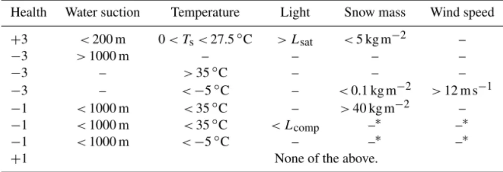
In order to determine the presence of moss in any grid cell, the model takes account of the local temperature, moisture, light, snow cover and, in some cases, wind speed (see Ta-ble 1). The moss cover is then determined by a “health” vari-able, whose value is updated once a day depending on the conditions over the past 24 h. Good conditions add to health and bad conditions subtract from it. It is contrained within
Figure 1. Soil carbon profiles generated using Eq. (1). Left: 119.75◦E, 72.25◦N; a grid cell with high soil carbon (Siberia). Right:−70.25◦E, 4.25◦N; a warm location with most of the carbon
near the surface (South America).
bounds that result in maximum health within a year given optimum growing conditions. The conditions for good and poor growth are given in Table 1. The water suction is taken as the minimum of water suctions in the top soil layer and the atmosphere, the temperature,Ts, is that of the top soil layer,
and the light is the radiation at the bottom of the canopy. These values are chosen for being closest to the soil surface where moss is located.
The temperature, moisture and light ranges for good growth are based on the values in Proctor (1982). The light saturation and compensation curves (LsatandLcomp
respec-tively) were estimated from Proctor (1982) and are given by
Lsat=19+exp(0.161Ts), (2)
Lcomp=0.1 exp(−0.5Ts)+0.4 exp(0.13Ts), (3)
where light compensation is the level at which photosynthe-sis balances respiration, and light saturation is the level at which photosynthesis is no longer light limited (increasing radiation levels no longer increase the rate of photosynthe-sis).
The heat and moisture conditions that cause the moss to die off are also taken from Proctor (1982). As well as dying in very hot or dry conditions, moss can suffer badly from wind damage when it is frozen (Longton, 1982). Thus the model includes a third scenario in which moss dies off: when it is cold, windy and there is no protective snow cover.
Table 1.Conditions for moss growth and dieback. For light saturation and compensation curves (LsatandLcomp) see Eqs. (2) and (3).
Health Water suction Temperature Light Snow mass Wind speed
+3 <200 m 0< Ts<27.5◦C > L
sat <5 kg m−2 –
−3 >1000 m – – – –
−3 – >35◦C – – –
−3 – <−5◦C – <0.1 kg m−2 >12 m s−1 −1 <1000 m <35◦C – >40 kg m−2 – −1 <1000 m <35◦C < L
comp –∗ –∗
−1 <1000 m <−5◦C – –∗ –∗
+1 None of the above.
∗Must not simultaneously satisfy snow mass<0.1 kg m−2, wind speed>12 m s−1and temperature<−5◦C.
based on snow mass values in JULES 2 weeks before the end of snowmelt. The magnitude of the values added to and subtracted from the health variable were calibrated at several sites where the moss cover was known.
When the moss health is positive, it is taken to have max-imum cover in the grid cell. When the health becomes neg-ative, the percentage cover drops off linearly to 0, and the cover is 0 for the lowest quartile of health values. If there is other vegetation present, the fractional cover of moss is capped at 0.7 for those vegetation tiles. This value was
prag-matically chosen given that moss can have around 50–100 % cover in forests (Beringer et al., 2001). Moss cover is as-sumed to be 0 for the urban or ice fraction of a grid box. The relationship of moss health to moss cover would benefit from further calibration.
Figure 2 shows a moss distribution simulated by JULES in the northern high latitudes and compares it with data from the Euskirchen et al. (2007) land-cover map. In general the most densely moss-covered areas correspond to the tundra land-cover classes, which are shown in bright green. Our scheme gives some general representation of this low veg-etation cover, which is otherwise missing in JULES. Moss also grows in the boreal forest (shown in purple on the Eu-skirchen map), but in JULES it does not grow in the decidu-ous needleleaf zone, which may require some investigation. Evaluating the distribution in lower latitudes is a subject for future work.
2.4 Data sets for model forcing and evaluation 2.4.1 Historical meteorological forcing data
The Water and Global Change (WATCH) project produced a meteorological forcing data set (WATCH Forcing Data Era-Interim, WFDEI) for use with land-surface and hydrologi-cal models (Weedon et al., 2010, 2011; Weedon, 2013). It is based on Era-Interim reanalysis data (ECMWF, 2009), with corrections generated from Climate Research Unit (Mitchell and Jones, 2005) and Global Precipitation Climatology Cen-tre data (http://gpcc.dwd.de). It covers the time period 1979– 2012 at half-degree resolution globally and at 3 hourly
tem-Figure 2.Upper plot: land-cover map using data from Euskirchen et al. (2007). “Shrub tundra” includes prostrate, dwarf shrub and low shrub tundra, and “boreal forest” includes boreal evergreen needleleaf and boreal broadleaf deciduous. Lower plot: mean moss cover simulated in JULES for the year 2000, from orgmossD his-torical simulation (see Table 2).
Table 2.List of JULES simulations carried out.
Simulation Soil Soil Bedrock Moss Organic Modified
layers depth soils snow
min4l 4 3 m N N N N
min14l 14 3 m N N N N
minD 28 10 m 50 m N N N
minmossD 28 10 m 50 m Y N N
orgD 28 10 m 50 m N Y N
orgmossD 28 10 m 50 m Y Y N
orgmossDS 28 10 m 50 m Y Y Y
poral resolution. Rainfall and snowfall are provided as sepa-rate variables.
2.4.2 Future meteorological forcing data
Meteorological forcing for the years 2006–2100 was created by adding modelled future climate anomalies to the histori-cal meteorologihistori-cal forcing. The monthly climate anomalies are from version 4 of the Community Climate System Model (CCSM4) and available at a resolution of 0.9◦latitude
×
1.25◦longitude. These were provided for the permafrost
pro-2020 2040 2060 2080 2100
−2
0
2
4
6
8
10
12
Year
Air temper
ature anomaly (
°
C) RCP 4.5
RCP 8.5
2020 2040 2060 2080 2100
0.8
1.0
1.2
1.4
1.6
1.8
Year
Precipitation scale f
actor
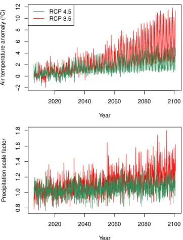
Figure 3.CCSM4 anomalies for air temperature and precipitation. Values given are the areal mean for the region north of 25◦latitude (the same region as the JULES simulations).
vided, including a combined precipitation variable rather than separate rain and snow, for two future scenarios – RCP4.5 and RCP8.5. As described in the protocol for the permafrost carbon MIP, these anomalies are combined with historical data either by addition (temperature, pressure, hu-midity, wind speed) or multiplication (short-wave and long-wave radiation, precipitation). The anomalies for air temper-ature and precipitation are shown in Fig. 3. There is not a large trend in precipitation, although in RCP8.5 there is a small increase, along with an increase in variability. Air tem-perature, however, shows a clear increase by the end of the century, up to 10◦C in RCP8.5. The change in air
tempera-ture is much larger in winter than in summer.
For the simulations discussed in this paper, the anomalies were re-gridded to 0.5◦resolution and applied to a repeating
sequence of 8 years of WFDEI reanalysis data (1998–2005). Using anomalies rather than directly using climate model data makes the climate variability in the future simulations more consistent with the historical data. The main disadvan-tage is that small-scale features are not captured, since sub-monthly variability comes from the base data set (Hempel et al., 2013).
2.4.3 CALM Network
The Circumpolar Active Layer Monitoring Network (CALM) (Brown et al., 2000, 2003) is a network of over 100 sites at which on-going measurements of the end-of-season thaw depth (the ALT) are taken. Mea-surements are available from the early 1990s, when the network was formed. The data are available from http://www.gwu.edu/~calm/data/north.html.
2.4.4 Historical soil temperatures
The Russian historical soil temperature data set is described in Frauenfeld et al. (2004). Soil temperatures were measured at 242 stations, over different time periods starting as early as 1890. The measurements used in this paper were taken at depths of 0.2, 0.4, 0.8, 1.6 and 3.2 m using extraction thermometers, with additional measurements at 0.6, 1.2 and 2.4 m. At some of the sites the natural vegetation cover was removed and at others there is some possibility of site dis-turbance, however the majority of these measurement sites retained their natural vegetation and snow cover.
International Polar Year Thermal State of Permafrost (IPY-TSP) borehole inventory data were compiled in 2007–2009 from both new and existing boreholes, achieving a wide spa-tial coverage of soil temperature data (Romanovsky, 2010). Data are available in the most part from 2006 to 2009 at a daily resolution, with temperatures measured at a variety of depths.
2.4.5 Globsnow
The European Space Agency snow water equivalent (SWE) product, GlobSnow (Takala et al., 2011) covers the years 1978–2010 and is available on an EASE-Grid at 25 km resolution. GlobSnow is produced using a combination of satellite-based microwave radiometer and ground-based weather station data. The GlobSnow documentation (Luojus et al., 2013) records an exponentially increasing bias with larger snow mass, which is particularly significant at snow mass greater than 200 kg m−2.
2.4.6 Permafrost distribution data
The Circum-Arctic map of permafrost and ground-ice condi-tions (Brown et al., 1998) gives a historical permafrost dis-tribution, which can be compared with permafrost area in the model. The data set contains information on the distri-bution and properties of permafrost and ground ice in the Northern Hemisphere (20–90◦N), with gridded data
avail-able at 12.5, 25 km and 0.5◦resolution. It records continuous,
would be simulated in the whole of the continuous and dis-continuous area, plus a fraction of permafrost in the areas of sporadic permafrost and isolated patches – the fractions be-ing 0.05 and 0.3 respectively. For the minimum we assume that no permafrost would be found in the sporadic and iso-lated regions and that in the continuous and discontinuous zones only a fractional coverage of permafrost is found: 0.95 and 0.7 respectively for the two zones. This gives a maximum area of 17.0 million km2and a minimum of 13.7 million km2. It is important to note that there is considerable uncertainty in these data which means that the true value could fall outside of this estimate.
2.5 Simulation set-up
For the historical period, JULES was driven by the WFDEI reanalysis data at a resolution of 0.5◦ (Sect. 2.4.1). JULES
was driven by precipitation (sum of rain and snow in WFDEI), which was converted internally within the model to rain and snow. This maintains consistency with the future driving data. The model was spun up for 60 years by repeat-ing the first 10 years of drivrepeat-ing data (1979–1988) and then run over the period 1979–2009 for the historical runs. Af-ter spin-up, the soil temperature and moisture contents were fully stabilised at the vast majority of points, i.e. there was no residual model drift. The future runs began at the start of 2006, taking their initial state from 2006 in the historical sim-ulations and simulating both RCP4.5 and RCP8.5 scenarios until 2100.
In order to capture all the main permafrost regions in the Northern Hemisphere, the simulations were run for the re-gion north of 25◦. The mineral soil properties, land-cover
fractions and topographic index data (needed for LSH, see Sect. 2.1) were taken from HadGEM2-ES ancillary data (Collins et al., 2008). Organic soil ancillaries were generated using the method described in Chadburn et al. (2015), with the spatial distribution as described in Sect. 2.3.1.
The simulations carried out are given in Table 2. This includes the standard JULES set-up (min4l), a higher-resolution soil column (min14l), a deeper soil column (minD), the effects of moss and organic soils both separately and in combination (minmossD, orgD, orgmossD) and finally the modified snow scheme (orgmossDS). When deeper soil is added in minD, this includes both the extension of the soil column to 10 m and the addition of a 50 m bedrock column. The distribution of moss was determined dynamically in the model as described in Sect. 2.3.2.
2.6 Evaluation methods
The maximum summer thaw depth or ALT was calculated by taking the unfrozen water fraction in the deepest layer that has begun to thaw and assuming that this same fraction of the soil layer has thawed. This gives significantly more
precise estimates of the ALT than temperature interpolation (see Chadburn et al., 2015).
The ALT was then used to derive the near-surface per-mafrost extent. Our definition of near-surface perper-mafrost is a grid cell with ALT less than 3 m for 2 or more consecutive years. There is no representation of sub-grid heterogeneity in the soils so any 0.5◦grid cell either contains 100 %
near-surface permafrost or no near-near-surface permafrost at all. Koven et al. (2012) calculated a range of metrics for soil temperature dynamics, which are also used here. They in-clude the offset between the mean air, 0 and 1 m tempera-tures and the attenuation of the annual cycle between each of these levels. The values were calculated as in Koven et al. (2012) by first calculating the annual mean and seasonal cy-cle at the available depths and then interpolating these to 0 and 1 m depth. The annual cycle was interpolated between layers by assuming it falls off exponentially with depth. The model values were taken from the grid cell containing the measurement point. All IPY-TSP sites with sufficient data were used, along with the colder Russian soil temperature sites (those with a mean soil temperature below 0◦C as an
indicator of permafrost). This gives a total of 86 sites with reasonable circumpolar coverage (see Sect. 2.4.4 for descrip-tion of observadescrip-tional data).
In order to analyse future permafrost degradation, the sen-sitivity of near-surface permafrost area loss to climate warm-ing was calculated via a linear regression of near-surface per-mafrost area against the annual mean air temperature over the historical permafrost region (region defined by the observed map in Brown et al., 1998).
3 Results
3.1 Active layer and near-surface soil temperatures in historical simulation
In Figs. 4 and 5, the simulated ALT from the JULES sim-ulations (Sect. 2.5) is compared with observations from the CALM active layer monitoring programme (Sect. 2.4.3). The low resolution in min4l significantly impairs the capacity of the model to simulate the active layer. This was seen for the point site simulation in Chadburn et al. (2015) and is even clearer in these large-scale results: the active layer in min4l has very little variability and little apparent correlation with the observations (see Fig. 5a).
pro-Obs. min4l min14l minD minmossD orgD orgmossD
0.5
1.0
1.5
2.0
2.5
3.0
Activ
e la
y
er thickness (m)
orgmossDS
Figure 4.Simulated and observed range of active layer depths for CALM sites (Sect. 2.4.3). Black dots are means, the boxes shows the interquartile range (IQR) and the horizontal line is the median. The whiskers indicate the most extreme data point that is no more than 1.5 times the IQR. Outliers are not shown. Points at which either the simulated or observed active layer was very large (greater than 6 m) were removed. The model point for each CALM site is the grid box containing that site.
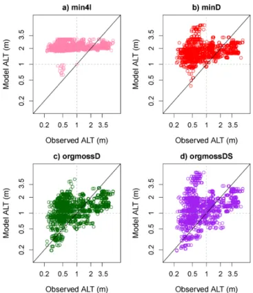
Figure 5.Active layer model values plotted against measurements
from CALM data set (as in Fig. 4). The dashed lines show an ALT of 1 m. Logarithmic axes are used.
cesses, the full range of ALT values are captured and the points fall around the one-to-one line. There is still an out-lying block of points where the active layer in JULES is greater than 3.5 m and much deeper than the measurements. Many of these sites fall along the course of the Mackenzie River in northern Canada (where JULES simulates very lit-tle permafrost – see Fig. 7). Precipitation gauges are sparse in this region so there may be large uncertainties in
hydrol-ogy (Weedon et al., 2011), and the observed soil tempera-tures vary greatly from around −1 to−7◦C as a result of
various influences including land cover and snow (Burn and Kokelj, 2009). This is a subject for future investigation.
The active layer thickness is determined by both the annual cycle of soil temperatures and the thermal offset between the air and the soil. Table 3 compares these dynamics in JULES with observations from the IPY-TSP data set and cold sites from the Russian soil temperature data set (see Sects. 2.4.4 and 2.6). The root mean squared error (RMSE) is calculated using the mean value of the metric for each site, so it quan-tifies the extent to which the variability between the sites is correctly simulated. In this table the most relevant values are the offset and attenuation of the annual cycle between the air and 1 m depth in the soil, since the soil surface is not so well defined in the observations. In the standard JULES set-up (min4l) the total offset is approximately correct, suggesting that the mean soil temperatures are simulated well. However, the annual cycle is nearly 25 % too large at 1 m depth.
The introduction of a well-resolved soil has a cooling ef-fect of approximately 0.7◦C, and organic soils and moss
have a further cooling effect of approximately 1◦C. As
in Chadburn et al. (2015), the improvements to the snow scheme then compensate for the cooling from the other model changes, resulting in a 1 m ground temperature ap-proximately the same in the final simulation (orgmossDS) as the original one (min4l). There is no significant improvement in the RMSE between the first and last simulation (quantify-ing the extent to which we capture the spatial variability), but the RMSE is between 2 and 2.5◦C for all simulations,
sug-gesting that the mean soil temperatures are captured fairly accurately.
The annual cycle, however, is reduced overall by the model improvements, with the attenuation value in orgmossDS be-ing very close to the observed value (less than 2 % different to be exact). The RMSE in these values is also reduced (by approximately 20 %) by the model developments, showing that spatial patterns are better simulated. This shows a sig-nificant improvement in the simulation.
Figure 6 shows the mean annual cycle of soil temperatures at 90 cm for the sites used in Table 3. Figure 6a shows that the main effect of increasing soil resolution is to reduce the winter temperatures. This is very likely because of the way the snow is simulated in the standard snow scheme, where the insulating effect of shallow snow is incorporated into the top soil layer – this means that when the top soil layer is thinner the insulation will be less effective. The deeper soil gives a slight attenuation of the annual cycle, which is expected of an additional heat sink.
re-Table 3.The attenuation of the annual cycle and the thermal offset in the JULES simulations, between the air and the top of the soil, and the top of the soil and 1 m depth, calculated as in Koven et al. (2012). This includes IPY-TSP and Russian data for cold sites. The RMSE (root mean squared error) values are based on the mean value of the metric at each site and thus give an indication of how well the variability between sites is captured. The bold numbers mark the observations as distinct from simulated values.
Simulation Attenuation (fraction of amplitude) Offset (◦C)
Air–0 m 0–1 m Total RMSE Air–0 m 0–1 m Total RMSE
Observations 0.62 0.40 0.25 – 7.7 −0.25 7.4 –
min4l 0.62 0.50 0.31 0.18 8.5 −1.00 7.5 2.5
min14l 0.67 0.52 0.35 0.20 7.3 −0.57 6.8 2.3
minD 0.68 0.48 0.33 0.20 7.4 −0.72 6.7 2.2
minmossD 0.66 0.48 0.32 0.18 7.2 −0.68 6.5 2.2
orgD 0.65 0.45 0.29 0.17 6.9 −0.92 6.0 2.4
orgmossD 0.62 0.45 0.28 0.16 6.7 −0.87 5.8 2.5
orgmossDS 0.54 0.47 0.25 0.15 8.1 −0.87 7.3 2.4
Figure 6.Comparison of annual cycle of soil temperatures at 90 cm depth, from the Russian historical soil temperature and IPY-TSP data (Sect. 2.4.4) and JULES simulations.
duced annual cycle which matches better with the observa-tions in Fig. 6c.
There are still significant differences between the model and observations, shown by the size of the RMSE in Table 3. The error in winter snow depth when compared with the clos-est grid cells in the Globsnow data set (see Sect. 2.4.5) has a significant correlation of 0.3 (for about 260 points) with the error in winter soil temperatures in orgmossDS, suggest-ing that snow explains at least some of the remainsuggest-ing error. Langer et al. (2013) show that uncertainty in the simulated active layer depth comes from the uncertainty in soil compo-sition, particularly ground-ice contents. Some variability is also expected when comparing a large grid cell with a point site, and this is difficult to quantify. While the RMSE in
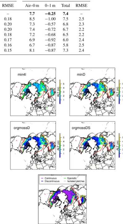
off-Figure 7.First two rows: mean active layer thickness in JULES simulations, 1979–1989. All grid cells with active layer≤6 m are
set is reasonably small, the RMSE for the attenuation of the annual cycle is a significant fraction of the value itself. This suggests that the annual cycle is more difficult to simulate than the mean temperature.
In this section a comparison with CALM observations has shown that one essential feature for simulating the ALT is the resolution of the soil column, without which the active layer variability is not resolved (see Fig. 4). For capturing the near-surface soil temperature dynamics, the effects of or-ganic soils and the improved snow scheme are both particu-larly significant in making the annual temperature cycle more realistic (Fig. 6 and Table 3). Organic soils also greatly im-prove the ALT (Figs. 4 and 5), so this process is a particularly useful addition to the model. The importance of organic soils has also been shown in e.g. Rinke et al. (2008); Lawrence et al. (2008); Koven et al. (2009).
3.2 Permafrost distribution in historical simulation The simulated permafrost in JULES is shown in Fig. 7, along with observations from the Circum-Arctic map of permafrost and ground-ice conditions (Brown et al., 1998) (Sect. 2.4.6). The observed map shows areas with continuous, discontin-uous and sporadic permafrost and isolated patches. There is no equivalent of discontinuous permafrost in JULES be-cause each grid box has only a single soil column, so in or-der to compare the two maps we assume that a deeper active layer in JULES may correspond to discontinuous or sporadic permafrost. With this assumption, all the simulations match the observations fairly well in most areas. We can see that introducing the model developments brings in much more spatial variability in ALT, which generally matches with the patterns of continuous/discontinuous permafrost. The corre-lation between the ALT in JULES and the percentage cover of permafrost from (Brown et al., 1998) (100 % for continu-ous, 90 % for discontinucontinu-ous, 50 % for sporadic and 10 % for isolated patches) is high, ranging between−0.37 and−0.51.
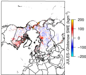
However, there are still places where continuous per-mafrost is observed but JULES does not simulate perper-mafrost. Figure 8 shows that in most of these areas, JULES simulates far too much snow, which will mean too much insulation in winter leading to soils that are too warm. This is particularly noticeable in north-east Canada and two areas in north-west Russia. In north-east Canada, however, it has been shown that the GlobSnow data set underestimates the SWE (Langlois et al., 2014), so the over-estimation in JULES may not be as large as Fig. 8 suggests. However, the permafrost in this re-gion is unstable to thawing (Thibault and Payette, 2009), so a small bias in the model could make the difference between simulating permafrost or not. For most of the remaining land surface, JULES slightly underestimates the SWE. Hancock et al. (2014) showed that JULES generally underestimates SWE when driven by reanalysis data sets.
In the observations, the edge of the permafrost-affected zone corresponds quite closely with the 0◦ isotherm,
al-Figure 8.Comparison of Globsnow and JULES. Mean snow
wa-ter equivalent (SWE) in Globsnow was subtracted from the JULES values over the same time periods. See Sect. 2.4.5.
though there is a gap in western Russia (red lines in Fig. 7). In the JULES simulations this relationship is less consistent, suggesting more spatial heterogeneity in the relationship be-tween air and soil temperatures. For example, excessive snow cover such as that seen in north-east Canada in Fig. 8 could contribute to this effect.
It is also possible to consider the vertical distribution of permafrost. Figure 9 shows a breakdown of active layer depths for all near-surface permafrost points (a) and all points (b) in the simulations. The first thing that is clear from this plot is that the discretisation of the soil column has a very large effect on the simulation of permafrost. A series of kinks corresponding to the model discretisation is apparent in all the curves, which for the higher-resolution simulations does not significantly impact the overall shape of the curve, but for the low-resolution soil changes it almost beyond recogni-tion. For about 50 % of the near-surface permafrost points in min4l, the active layer depth is between 1.8 and 2.2 m, where 2 m is the centre of the bottom model layer.
0.0 0.2 0.4 0.6 0.8 1.0
Fraction of points
Activ
e la
y
er depth (m)
3
2
1
0 min4l
min14l minD orgmossD orgmossDS
a) Just near−surface permafrost points
0.7 0.8 0.9 1.0
Fraction of points
Activ
e la
y
er depth (m)
3
2
1
0
b) All points
Figure 9.The vertical distribution of permafrost, shown by the frac-tion of points for which the soil thaws below a given depth.(a) Near-surface permafrost points only: this includes only those points with ALT less than 3 m, and hence 0 % of them thaw to below 3 m.(b)All points are included, so about 70 % thaw to greater than 3 m or have no permafrost at all. There is one point for each grid cell for each year of the historical simulation.
the surface but warmer in the deeper soil. This is seen in the soil temperature profiles in Fig. 10.
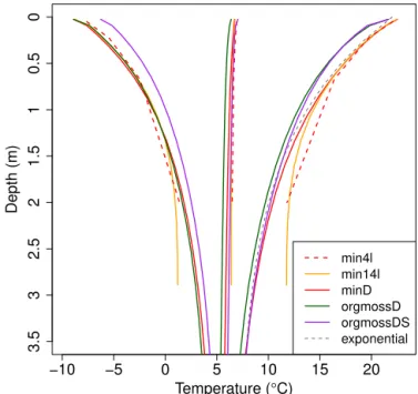
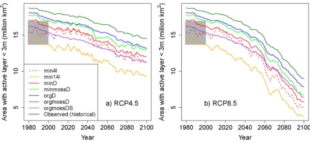
The total near-surface permafrost area in each simulation is more clearly seen by looking at the historical period in Fig. 11. For consistency with the definition of near-surface permafrost, these values include any grid cells where the ALT was less than 3 m for the past 2 years (so for exam-ple in the first year that a grid cell is frozen, it is not included in the permafrost area but after the second year it is added to the area, so the area changes from year to year). Com-paring the deep-soil simulations, minD, minmossD, orgD and orgmossD, we see that adding insulation from organic soils and moss increases the near-surface permafrost area, which is consistent with the cooling effect seen in Table 3. In orgmossDS, the near-surface permafrost area is significantly reduced compared with orgmossD, which was also apparent in Fig. 9b. Finally, in the shallow (3 m) simulations (min4l and min14l), the near-surface permafrost area is smaller, but this is not really meaningful. This is because the zero-heat-flux boundary condition is not correct at 3 m, which leads to “edge effects” close to the soil boundary. This is seen in Fig. 10, where the soil temperatures in the mineral soil sim-ulations (min4l, min14l and minD) are very similar near the top of the soil, but the annual cycle in the shallow simulations (min4l and min14l) does not continue to fall off with depth, resulting in a maximum temperature that is much too high at the base of the soil. This shows that diagnosing permafrost as the area with ALT less than 3 m requires a soil column significantly deeper than 3 m.
A range for the observed permafrost area is also shown in Fig. 11. This is estimated from Brown et al. (1998) us-ing assumptions described in Sect. 2.4.6. Accordus-ing to this, the simulated near-surface permafrost area in the mineral soil
−10 −5 0 5 10 15 20
Temperature (°C)
Depth (m)
3.5
3
2.5
2
1.5
1
0.5
0
min4l min14l minD orgmossD orgmossDS exponential
Figure 10.The annual maximum, minimum and mean of
simu-lated soil temperatures (right-hand, left-hand and centre lines re-spectively), averaged over the period 1979–1989, for the land area north of 50◦latitude. Comparing the simulations with different soil depth is of particular interest here.
simulations (min4l, min14l, minD) falls inside the observed range, and the addition of organic soils and moss results in a simulated near-surface permafrost area that is somewhat too large. However, in the final simulation with all model im-provements (orgmossDS), the near-surface permafrost area once again falls within the observed range.
3.3 Future permafrost degradation
Section 3.1 showed that the model improvements make the simulation of permafrost more realistic. Although further de-velopment is needed, these are important processes to in-clude and it is worthwhile to study their impact on long-term permafrost dynamics; hence in this section we study the loss of near-surface permafrost and the active layer deepen-ing over the next century.
Figure 11.Time series of future projections of permafrost area. Left: RCP4.5. Right: RCP8.5. The grey area represents an estimate of the observed area from Brown et al. (1998) (see Sect. 2.4.6).
Table 4.Rate of loss of near-surface permafrost per degree of high-latitude warming in future JULES simulations. The temperature change is calculated over the historical permafrost area (observed).
Simulation Historical area Rate of loss (106km2◦C−1) Rate of loss (fraction◦C−1)
(106km2) RCP4.5 RCP8.5 RCP4.5 RCP8.5
min4l 15.5 −1.52 −1.47 0.101 0.097
min14l 14.3 −1.36 −1.32 0.106 0.101
minD 17.0 −1.34 −1.37 0.085 0.087
minmossD 17.7 −1.33 −1.34 0.080 0.080
orgD 18.0 −1.17 −1.21 0.069 0.071
orgmossD 18.7 −1.08 −1.19 0.060 0.066
orgmossDS 16.1 −1.15 −1.11 0.077 0.074
HadGEM2-ES 22–23a −1.5a −1.46b 0.065a
aKoven et al. (2012),bSlater and Lawrence (2013).
deep soil simulations, indicating the importance of the ther-mal inertia from a deep heat sink in the soil, which has been shown already in e.g. Stevens et al. (2007); Alexeev et al. (2007); Lawrence et al. (2008).
Table 4 shows the rate of near-surface permafrost loss per degree of warming (calculated by a linear regression between future mean air temperature, averaged over the historical per-mafrost region, and perper-mafrost area). The sensitivity is re-duced by the new model developments, from approximately 1.5×10⁶km2◦C−1in the standard JULES set-up (min4l) to
between 1.1×10⁶ and 1.2×10⁶km2◦C−1 in orgmossDS:
a reduction of about 25 %. In Lawrence et al. (2008) the rate of permafrost loss in the Community Land Model is reduced by over 25 % by the inclusion of organic matter and a deeper soil column, which is an even larger effect than is found in JULES. In that study an even deeper soil column down to 125 m was used.
The loss of near-surface permafrost by the end of the 21st century is very large in all the JULES simulations, partic-ularly in RCP8.5. Even in orgmossD and orgmossDS, the simulations with the lowest sensitivity to temperature, the
area with near-surface permafrost has approximately halved by the end of the 21st century in RCP8.5 (see Fig. 11). In orgmossDS it decreases from approximately 16 million km2 for the historical period down to approximately 7 million km2 in RCP8.5 and 12 million km2in RCP4.5 by 2100.
Figure 12.Coloured area shows near-surface permafrost at the start of the simulation: green regions have disappeared by the end of the simulation (2090–2100) and other colours (reddish) show active layer deepening in the remaining permafrost.
0.43 million km2. Compared with the other CMIP5 models, the rates of near-surface permafrost loss in the improved ver-sion of JULES (orgmossDS) are now lower than most of the other models (Koven et al., 2012; Slater and Lawrence, 2013).
Figure 12 shows the near-surface permafrost distribu-tion at the end of the future simuladistribu-tions for the “standard” JULES set-up (min4l) and the final improved model version (orgmossDS). In RCP4.5 the near-surface permafrost retreats only from the edges of the permafrost zone, but there is some thickening of the active layer across the whole near-surface permafrost area of the order of 0.5 m, which is a significant change. In the more southern permafrost regions, the active layer deepens more in orgmossDS – as much as 1 m – which may reflect the fact that the ALT is initially shallower, so more deepening is possible.
In RCP8.5, much of the near-surface permafrost thaws in both simulations. However, in the improved model version, there is significantly more near-surface permafrost remain-ing at the end of the century, particularly in northern Russia, reflecting the reduced sensitivity to warming. However, the areas where near-surface permafrost remains in orgmossDS show a strong active layer deepening, significantly more than 1 m in some areas. This suggests that although less near-surface permafrost is lost in this simulation, with a further
in-crease in temperature it could disappear. Note that this refers just to permafrost at depths of up to 3 m – deeper permafrost may remain longer.
4 Conclusions
Large-scale simulations have shown improved physical per-mafrost dynamics in JULES, thanks to a deeper and better-resolved soil column, including the physical effects of moss and organic soils and an improvement to the snow scheme. The model developments reduce the simulated summer thaw depth and the amplitude of the annual cycle of soil tempera-tures and bring both to more realistic values. The rate of near-surface permafrost loss under future climate warming is also reduced, as is the interannual variability of the near-surface permafrost area.
A well-resolved soil is absolutely essential for simulating active layer dynamics. With a poorly resolved soil it is not possible to simulate ALT variability: the thaw depth depends strongly on the model layers, Fig. 9, and there is very little spatial variability in ALT (Fig. 7), which is unrealistic (see Fig. 5). The importance of soil resolution has not often been emphasised in the literature.
We have confirmed the importance of including a deep soil column, showing that the thermal inertia from deeper soil has a significant impact on the permafrost dynamics (see e.g. Figs. 4 and 11). We also find that with a 3 m soil column it is not possible to meaningfully diagnose permafrost at 3 m depth due to the edge effects close to the bottom boundary of the soil (Fig. 10).
Organic soils and moss both act to insulate the soil. They reduce the ALT and increase the near-surface permafrost area (see for example Fig. 4 and Table 4) due to their insulating effect in summer, which helps to make the annual cycle of soil temperatures more realistic (Fig. 6b). Of these two pro-cesses, organic soils have the larger effect. Including moss has a smaller but significant physical impact, as seen for example by the increase in near-surface permafrost area of 0.7 million km2when it is included (Table 4). High-latitude vegetation is an important component that is currently miss-ing in JULES. This simple insulatmiss-ing layer is only the first step and more work is needed to fully incorporate it into the vegetation model.
The improvement to the snow scheme has a large winter warming effect (Fig. 6c), and as a result it warms the deep soil and reduces the near-surface permafrost area, bringing it closer to the observational estimate. It also contributes to a more realistic annual cycle (Fig. 6c). However, the snow is less important for simulating the correct ALT (Fig. 5).
Snow has a very strong effect on soil temperatures (West-ermann et al., 2013; Ekici et al., 2015; Langer et al., 2013), and there is certainly more scope to improve the snow model in JULES, for example with additional compaction processes and lateral redistribution. However, there are high uncertain-ties associated with global precipitation data in observations, reanalysis products and climate model output, particularly for the Arctic (Bosilovich et al., 2008; Kattsov et al., 2007; Hancock et al., 2014), so these limit the potential to improve the snow representation at present.
Soil moisture is also important for soil temperatures, and the two are linked in a complex manner. Water has a higher thermal conductivity than air, so in wetter soils more heat will penetrate and leave the ground. However, if there is soil freezing and thawing, the latent heat will reduce the rate of heat penetration, counteracting this effect. Furthermore, if there is soil freezing the mean temperature in the deeper soil is colder than that at the surface, since the thermal conductiv-ity of ice is greater than that of water, so more heat moves up-wards in winter than downup-wards in summer. The influence of soil temperature on soil moisture mainly comes from
freez-ing, as this prevents moisture running out of the soil and may also hold liquid water above a permafrost layer.
Between the runs in this paper, the main differences in soil moisture come from organic soils, which increase the soil moisture content overall. Disentangling the complex im-pacts requires more specific experiments than the ones in this study, such as an experiment where specific influences of soil moisture on temperature are removed. Further investigation of the hydrology in JULES is vital and this is the subject of ongoing work.
Important improvements have been made in JULES and other global land-surface models (e.g. Lawrence and Slater, 2008; Gouttevin et al., 2012a; Ekici et al., 2014), but these models are now somewhat limited by their coarse spatial resolution, since permafrost processes are heterogeneous on small spatial scales and have non-linear effects. There is some progress being made towards upscaling small-scale processes (Muster et al., 2012; Langer et al., 2013), and large-scale data sets are improving over time, which is im-portant for simulating realistic carbon fluxes.
In this paper we have analysed the large-scale degradation of permafrost under two future climate scenarios. This shows a significant reduction in near-surface permafrost area, with up to 1.5 million km2of near-surface permafrost loss per de-gree of high-latitude warming, although this is reduced to approximately 1.1 million km2 in the improved model ver-sion, showing the importance of these model developments in assessing future permafrost thaw. The impact of organic matter is particularly large, as this alone reduces the sen-sitivity by approximately 15 % (Table 4). In RCP4.5, near-surface permafrost is only lost from the edges of the per-mafrost zone by the end of the century, but in RCP8.5 the near-surface permafrost disappears entirely from some large regions, with large areas of near-surface permafrost remain-ing only in northern Canada and some parts of Russia. In areas where near-surface permafrost remains, there is a sig-nificant thickening of the active layer, which is relevant for consideration of the permafrost carbon feedback.
Acknowledgements. The authors acknowledge financial sup-port by the European Union Seventh Framework Programme (FP7/2007-2013) project PAGE21, under GA282700. E. Burke was supported by the joint UK DECC/Defra Met Office Hadley Centre Climate Programme GA01101. M. Langer is also supported by a post-doctoral research fellowship (A. v. Humboldt Foundation). We also thank the reviewers for their comments to improve the manuscript.
References
Alexeev, V. A., Nicolsky, D. J., Romanovsky, V. E., and Lawrence, D. M.: An evaluation of deep soil configurations in the CLM3 for improved representation of permafrost, Geophys. Res. Lett., 34, L09502, doi:10.1029/2007GL029536, 2007.
Bekryaev, R. V., Polyakov, I. V., and Alexeev, V. A.: Role of polar amplification in long-term surface air temperature varia-tions and modern arctic warming, J. Climate, 23, 3888–3906, doi:10.1175/2010JCLI3297.1, 2010.
Beringer, J., Lynch, A. H., Chapin, F. S., Mack, M., and Bonan, G. B.: The representation of Arctic soils in the Land Surface Model: the importance of mosses, J. Climate, 14, 3324–3335, doi:10.1175/1520-0442(2001)014<3324:TROASI>2.0.CO;2, 2001.
Best, M. J., Pryor, M., Clark, D. B., Rooney, G. G., Essery, R. L. H., Ménard, C. B., Edwards, J. M., Hendry, M. A., Porson, A., Gedney, N., Mercado, L. M., Sitch, S., Blyth, E., Boucher, O., Cox, P. M., Grimmond, C. S. B., and Harding, R. J.: The Joint UK Land Environment Simulator (JULES), model description – Part 1: Energy and water fluxes, Geosci. Model Dev., 4, 677–699, doi:10.5194/gmd-4-677-2011, 2011.
Bosilovich, M. G., Chen, J., Robertson, F. R., and Adler, R. F.: Eval-uation of global precipitation in reanalyses, J. Appl. Meteorol. Clim., 47, 2279–2299, doi:10.1175/2008JAMC1921.1, 2008. Brooks, R. and Corey, A.: Hydraulic Properties of Porous
Me-dia, Colorado State University Hydrology Papers, Colorado State University, available at: http://books.google.co.uk/books?id=F_ 1HOgAACAAJ, last access: 27 January 2015, 1964.
Brown, J., Ferrians Jr., O. J., Heginbottom, J., and Melnikov, E.: Circum-arctic map of permafrost and ground ice conditions, Na-tional Snow and Ice Data Center, available at: http://nsidc.org/ data/docs/fgdc/ggd318_map_circumarctic, last access: 27 Jan-uary 2015, 1998.
Brown, J., Nelson, F. E., and Hinkel, K. M.: The circumpolar active layer monitoring (CALM) program: research designs and initial results, Polar Geogr., 3, 165–258, 2000.
Brown, J., Hinkel, K. M., and Nelson, F. E.: Circumpolar Active Layer Monitoring (CALM) Program Network, National Snow and Ice Data Center, Boulder, Colorado USA, 2003.
Burke, E., Dankers, R., Jones, C., and Wiltshire, A.: A retrospective analysis of pan Arctic permafrost using the JULES land surface model, Clim. Dynam., 41, 1025–1038, doi:10.1007/s00382-012-1648-x, 2013.
Burke, E. J., Hartley, I. P., and Jones, C. D.: Uncertainties in the global temperature change caused by carbon release from per-mafrost thawing, The Cryosphere, 6, 1063–1076, doi:10.5194/tc-6-1063-2012, 2012.
Burn, C. R. and Kokelj, S. V.: The environment and permafrost of the Mackenzie Delta area, Permafrost Periglac., 20, 83–105, doi:10.1002/ppp.655, 2009.
Camill, P.: Permafrost thaw accelerates in boreal peatlands during late-20th century climate warming, Climatic Change, 68, 135– 152, doi:10.1007/s10584-005-4785-y, 2005.
Chadburn, S., Burke, E., Essery, R., Boike, J., Langer, M., Heiken-feld, M., Cox, P., and Friedlingstein, P.: An improved representa-tion of physical permafrost dynamics in the JULES land-surface model, Geosci. Model Dev., 8, 1493–1508, doi:10.5194/gmd-8-1493-2015, 2015.
Clark, D. B., Mercado, L. M., Sitch, S., Jones, C. D., Gedney, N., Best, M. J., Pryor, M., Rooney, G. G., Essery, R. L. H., Blyth, E., Boucher, O., Harding, R. J., Huntingford, C., and Cox, P. M.: The Joint UK Land Environment Simulator (JULES), model descrip-tion – Part 2: Carbon fluxes and vegetadescrip-tion dynamics, Geosci. Model Dev., 4, 701–722, doi:10.5194/gmd-4-701-2011, 2011. Collins, N. J. and Callaghan, T. V.: Predicted patterns of
photo-synthetic production in maritime Antarctic mosses, Ann. Bot.-London, 45, 601–620, 1980.
Collins, W., Bellouin, N., Doutriaux-Boucher, M., Gedney, N., Hin-ton, T., Jones, C. D., Liddicoat, S., Martin, G., O’Connor, F., Rae, J., Senior, C., Totterdell, I., Woodward, S., Reichler, T., and Kim, J.: Evaluation of the HadGEM2 model, Met Office Hadley Centre Technical Note no. HCTN 74, Met Office, FitzRoy Road, Exeter, UK, available at: http://www.metoffice.gov.uk/archive/science/ climate-science/hctn74, last access: 27 January 2015, 2008. Comiso, J. C.: Large decadal decline of the Arctic multiyear
ice cover, J. Climate, 25, 1176–1193, doi:10.1175/JCLI-D-11-00113.1, 2012.
Cosby, B. J., Hornberger, G. M., Clapp, R. B., and Ginn, T. R.: A statistical exploration of the relationships of soil moisture char-acteristics to the physical properties of soils, Water Resour. Res., 20, 682–690, doi:10.1029/WR020i006p00682, 1984.
Cox, P. M., Betts, R. A., Bunton, C. B., Essery, R. L. H., Rown-tree, P. R., and Smith, J.: The impact of new land surface physics on the GCM simulation of climate and climate sensitivity, Clim. Dynam., 15, 183–203, doi:10.1007/s003820050276, 1999. Dankers, R., Burke, E. J., and Price, J.: Simulation of permafrost
and seasonal thaw depth in the JULES land surface scheme, The Cryosphere, 5, 773–790, doi:10.5194/tc-5-773-2011, 2011. Dharssi, I., Vidale, P., Verhoef, A., Macpherson, B., Jones,
C., and Best, M.: New soil physical properties imple-mented in the Unified Model at PS18, Meteorology Re-search and Development technical report 528, Met Of-fice, UK, available at: http://www.metoffice.gov.uk/archive/ forecasting-research-technical-report-528, last access: 20 March 2015, 2009.
ECMWF (European Center for Medium-Range Weather Forecasts) ECMWF ERA-40 Re-Analysis data, NCAS British Atmospheric Data Centre, available at: http://badc.nerc.ac.uk/view/badc.nerc. ac.uk_ATOM_dataent_12458543158227759, last access: 27 Jan-uary 2015, 2009.
Ekici, A., Beer, C., Hagemann, S., Boike, J., Langer, M., and Hauck, C.: Simulating high-latitude permafrost regions by the JSBACH terrestrial ecosystem model, Geosci. Model Dev., 7, 631–647, doi:10.5194/gmd-7-631-2014, 2014.
Ekici, A., Chadburn, S., Chaudhary, N., Hajdu, L. H., Marmy, A., Peng, S., Boike, J., Burke, E., Friend, A. D., Hauck, C., Krin-ner, G., Langer, M., Miller, P. A., and Beer, C.: Site-level model intercomparison of high latitude and high altitude soil thermal dynamics in tundra and barren landscapes, The Cryosphere, 9, 1343–1361, doi:10.5194/tc-9-1343-2015, 2015.
Essery, R., Best, M., Betts, R., and Taylor, C.: Explicit representa-tion of subgrid heterogeneity in a GCM land surface scheme, J. Hydrometeorol., 4, 530–543, 2003.
warm-ing, Glob. Change Biol., 13, 2425–2438, doi:10.1111/j.1365-2486.2007.01450.x, 2007.
FAO/IIASA/ISRIC/ISS-CAS/JRC: Harmonized World Soil Database (version 1.2), FAO, Rome, Italy and IIASA, Lax-enburg, Austria, available at: http://webarchive.iiasa.ac.at/ Research/LUC/External-World-soil-database/HTML/, last access: 20 January 2015, 2012.
Frauenfeld, O. W., Zhang, T., Barry, R. G., and Gilichinsky, D.: Interdecadal changes in seasonal freeze and thaw depths in Rus-sia, J. Geophys. Res., 109, D05101, doi:10.1029/2003JD004245, 2004.
Gedney, N. and Cox, P. M.: The sensitivity of global cli-mate model simulations to the representation of soil mois-ture, J. Hydrometeorol., 4, 1265–1275, doi:10.1175/1525-7541(2003)004<1265:TSOGCM>2.0.CO;2, 2003.
Gouttevin, I., Krinner, G., Ciais, P., Polcher, J., and Legout, C.: Multi-scale validation of a new soil freezing scheme for a land-surface model with physically-based hydrology, The Cryosphere, 6, 407–430, doi:10.5194/tc-6-407-2012, 2012a.
Gouttevin, I., Menegoz, M., Dominé, F., Krinner, G., Koven, C., Ciais, P., Tarnocai, C., and Boike, J.: How the insulat-ing properties of snow affect soil carbon distribution in the continental pan-Arctic area, J. Geophys. Res., 117, G02020, doi:10.1029/2011JG001916, 2012b.
Hancock, S., Huntley, B., Ellis, R., and Baxter, R.: Biases in reanal-ysis snowfall found by comparing the JULES land surface model to GlobSnow, J. Climate, 27, 624–632, doi:10.1175/JCLI-D-13-00382.1, 2014.
Harden, J. W., Koven, C. D., Ping, C.-L., Hugelius, G., David McGuire, A., Camill, P., Jorgenson, T., Kuhry, P., Michael-son, G. J., O’Donnell, J. A., Schuur, E. A. G., Tarnocai, C., John-son, K., and Grosse, G.: Field information links permafrost car-bon to physical vulnerabilities of thawing, Geophys. Res. Lett., 39, L15704, doi:10.1029/2012GL051958, 2012.
Hempel, S., Frieler, K., Warszawski, L., Schewe, J., and Piontek, F.: A trend-preserving bias correction – the ISI-MIP approach, Earth Syst. Dynam., 4, 219–236, doi:10.5194/esd-4-219-2013, 2013. Hugelius, G., Tarnocai, C., Broll, G., Canadell, J. G., Kuhry, P.,
and Swanson, D. K.: The Northern Circumpolar Soil Carbon Database: spatially distributed datasets of soil coverage and soil carbon storage in the northern permafrost regions, Earth Syst. Sci. Data, 5, 3–13, doi:10.5194/essd-5-3-2013, 2013.
Hugelius, G., Strauss, J., Zubrzycki, S., Harden, J. W., Schuur, E. A. G., Ping, C.-L., Schirrmeister, L., Grosse, G., Michaelson, G. J., Koven, C. D., O’Donnell, J. A., Elberling, B., Mishra, U., Camill, P., Yu, Z., Palmtag, J., and Kuhry, P.: Estimated stocks of circumpolar permafrost carbon with quantified uncertainty ranges and identified data gaps, Biogeosciences, 11, 6573–6593, doi:10.5194/bg-11-6573-2014, 2014.
Kattsov, V. M., Walsh, J. E., Chapman, W. L., Govorkova, V. A., Pavlova, T. V., and Zhang, X.: Simulation and pro-jection of Arctic freshwater budget components by the IPCC AR4 global climate models, J. Hydrometeorol., 8, 571–589, doi:10.1175/JHM575.1, 2007.
Koven, C., Friedlingstein, P., Ciais, P., Khvorostyanov, D., Krin-ner, G., and Tarnocai, C.: On the formation of high-latitude soil carbon stocks: effects of cryoturbation and insulation by organic matter in a land surface model, Geophys. Res. Lett., 36, L21501, doi:10.1029/2009GL040150, 2009.
Koven, C. D., Ringeval, B., Friedlingstein, P., Ciais, P., Cadule, P., Khvorostyanov, D., Krinner, G., and Tarnocai, C.: Permafrost carbon–climate feedbacks accelerate global warming, P. Natl. Acad. Sci. USA, 108, 14769–14774, doi:10.1073/pnas.1103910108, 2011.
Koven, C. D., Riley, W. J., and Stern, A.: Analysis of per-mafrost thermal dynamics and response to climate change in the CMIP5 Earth System Models, J. Climate, 26, 1877–1900, doi:10.1175/JCLI-D-12-00228.1, 2012.
Langer, M., Westermann, S., Heikenfeld, M., Dorn, W., and Boike, J.: Satellite-based modeling of permafrost temperatures in a tundra lowland landscape, Remote Sens. Environ., 135, 12–24, doi:10.1016/j.rse.2013.03.011, 2013.
Langlois, A., Bergeron, J., Brown, R., Royer, A., Harvey, R., Roy, A., Wang, L., and Thériault, N.: Evaluation of class 2.7 and 3.5 simulations of snow properties from the Canadian Regional Cli-mate Model (CRCM4) over Québec, Canada, J. Hydrometeor, 15, 1325–1343, doi:10.1175/JHM-D-13-055.1, 2014.
Lawrence, D. and Slater, A.: Incorporating organic soil into a global climate model, Clim. Dynam., 30, 145–160, doi:10.1007/s00382-007-0278-1, 2008.
Lawrence, D., Slater, A., Romanovsky, V., and Nicolsky, D.: Sensi-tivity of a model projection of near-surface permafrost degrada-tion to soil column depth and representadegrada-tion of soil organic mat-ter, J. Geophys. Res., 113, F02011, doi:10.1029/2007JF000883, 2008.
Longton, R. E.: Bryophyte vegetation in polar regions, in: Bryophyte Ecology, edited by: Smith, A., Springer, London, Chapman and Hall, 123–165, 1982.
Luojus, K., Pulliainen, J., Takala, M., Lemmetyinen, J., Kangwa, M., Smolander, T., and Derksen, C.: Algorithm Theoretical Basis Document – SWE-algorithm, Euro-pean Space Agency Study Contract Report, available at: www.globsnow.info/docs/GS2_SWE_ATBD.pdf, last access: 3 July 2015, 2013.
MacDougall, A. H., Avis, C. A., and Weaver, A. J.: Significant con-tribution to climate warming from the permafrost carbon feed-back, Nat. Geosci., 5, 719–721, doi:10.1038/ngeo1573, 2012. Mitchell, T. D. and Jones, P. D.: An improved method of
con-structing a database of monthly climate observations and as-sociated high-resolution grids, Int. J. Climatol., 25, 693–712, doi:10.1002/joc.1181, 2005.
Muster, S., Langer, M., Heim, B., Westermann, S., and Boike, J.: Subpixel heterogeneity of ice-wedge polygonal tundra: a multi-scale analysis of land cover and evapotranspiration in the Lena River Delta, Siberia, Tellus B, 64, 17301, doi:10.3402/tellusb.v64i0.17301, 2012.
Paquin, J.-P. and Sushama, L.: On the Arctic near-surface per-mafrost and climate sensitivities to soil and snow model for-mulations in climate models, Clim. Dynam., 44, 203–228, doi:10.1007/s00382-014-2185-6, 2014.
Proctor, M. C. F.: Physiological ecology: water relations, light and temperature responses, carbon balance, in: Bryophyte Ecology, edited by: Smith, A., Springer, London, Chapman and Hall, 333– 382, 1982.
Richards, L. A.: Capillary conduction of liquids through porous mediums, J. Appl. Phys., 1, 318–333, 1931.
Geophys. Res. Lett., 35, L13709, doi:10.1029/2008GL034052, 2008.
Romanovsky, V. E.: Development of a network of permafrost observatories in North America and Russia: the US contri-bution to the international polar year, Advanced Cooperative Arctic Data and Information Service, Boulder, CO, available at: https://www.aoncadis.org/project/development, last access: 20 March 2015, 2010.
Romanovsky, V. E., Drozdov, D. S., Oberman, N. G., Malkova, G. V., Kholodov, A. L., Marchenko, S. S., Moskalenko, N. G., Sergeev, D. O., Ukraintseva, N. G., Abramov, A. A., Gilichinsky, D. A., and Vasiliev, A. A.: Thermal state of permafrost in Russia, Permafrost Periglac., 21, 136–155, doi:10.1002/ppp.683, 2010. Schneider von Deimling, T., Meinshausen, M., Levermann, A.,
Hu-ber, V., Frieler, K., Lawrence, D. M., and Brovkin, V.: Estimating the near-surface permafrost-carbon feedback on global warming, Biogeosciences, 9, 649–665, doi:10.5194/bg-9-649-2012, 2012. Schneider von Deimling, T., Grosse, G., Strauss, J., Schirrmeis-ter, L., Morgenstern, A., Schaphoff, S., Meinshausen, M., and Boike, J.: Observation-based modelling of permafrost car-bon fluxes with accounting for deep carcar-bon deposits and thermokarst activity, Biogeosciences Discuss., 11, 16599–16643, doi:10.5194/bgd-11-16599-2014, 2014.
Schuur, E. A. G., Vogel, J. G., Crummer, K. G., Lee, H., Sickman, J. O., and Osterkamp, T. E.: The effect of permafrost thaw on old carbon release and net carbon exchange from tundra, Nature, 459, 556–559, doi:10.1038/nature08031, 2009.
Slater, A. G. and Lawrence, D. M.: Diagnosing present and fu-ture permafrost from climate models, J. Climate, 26, 5608–8755, doi:10.1175/JCLI-D-12-00341.1, 2013.
Soudzilovskaia, N. A., van Bodegom, P. M., and Cornelissen, J. H.: Dominant bryophyte control over high-latitude soil tempera-ture fluctuations predicted by heat transfer traits, field moistempera-ture regime and laws of thermal insulation, Funct. Ecol., 27, 1442– 1454, doi:10.1111/1365-2435.12127, 2013.
Stevens, M. B., Smerdon, J. E., González-Rouco, J. F., Stieglitz, M., and Beltrami, H.: Effects of bottom boundary placement on sub-surface heat storage: implications for climate model simulations, Geophys. Res. Lett., 34, L02702, doi:10.1029/2006GL028546, 2007.
Stocker, T., Qin, D., Plattner, G.-K., Tignor, M., Allen, S., Boschung, J., Nauels, A., Xia, Y., Bex, V., and Midgley, P. M. (Eds.): Climate Change 2013: The Physical Science Basis, in: Contribution of Working Group I to the Fifth Assessment Report of the Intergovernmental Panel on Climate Change, IPCC, Cambridge University Press, available at: http://www. climatechange2013.org/, last access: 27 January 2015, 2013.
Stroeve, J., Serreze, M., Holland, M., Kay, J., Malanik, J., and Barrett, A.: The Arctic’s rapidly shrinking sea ice cover: a research synthesis, Climatic Change, 110, 1005–1027, doi:10.1007/s10584-011-0101-1, 2012.
Takala, M., Luojus, K., Pulliainen, J., Derksen, C., Lemmetyi-nen, J., Kärnä, J.-P., KoskiLemmetyi-nen, J., and Bojkov, B.: Estimating northern hemisphere snow water equivalent for climate research through assimilation of space-borne radiometer data and ground-based measurements, Remote Sens. Environ., 115, 3517–3529, doi:10.1016/j.rse.2011.08.014, 2011.
Thibault, S. and Payette, S.: Recent permafrost degradation in bogs of the James Bay area, northern Quebec, Canada, Permafrost Periglac. Process., 20, 383–389, doi:10.1002/ppp.660, 2009. Weedon, G. P.: Readme file for the “WFDEI” dataset,
avail-able at: http://www.eu-watch.org/gfx_content/documents/ README-WFDEI.pdf, last access: 27 January 2015, 2013. Weedon, G. P., Gomes, S., Viterbo, P., Österle, H., Adam, J. C.,
Bellouin, N., Boucher, O., and Best., M.: The WATCH forc-ing data 1958–2001: a meteorological forcforc-ing dataset for land surface- and hydrological-models, WATCH technical report, p. 41, available at: http://www.eu-watch.org/publications, last ac-cess: 27 January 2015, 2010.
Weedon, G. P., Gomes, S., Viterbo, P., Shuttleworth, W. J., Blyth, E., Österle, H., Adam, J. C., Bellouin, N., Boucher, O., and Best, M.: Creation of the WATCH forcing data and its use to assess global and regional reference crop evaporation over land during the twentieth century, J. Hydrometeorol., 12, 823–847, doi:10.1175/2011JHM1369.1, 2011.
Westermann, S., Schuler, T. V., Gisnås, K., and Etzelmüller, B.: Transient thermal modeling of permafrost conditions in Southern Norway, The Cryosphere, 7, 719—739, doi:10.5194/tc-7-719-2013, 2013.