Modeling the impact of wintertime rain events on the thermal regime of permafrost

(1)

TCD

5, 1697–1736, 2011

Modeling wintertime rain events

S. Westermann et al.

Title Page

Abstract Introduction

Conclusions References

Tables Figures

◭ ◮

Back Close

Full Screen / Esc

Printer-friendly Version Interactive Discussion

Discussion

P

a

per

|

Dis

cussion

P

a

per

|

Discussion

P

a

per

|

Discussio

n

P

a

per

|

The Cryosphere Discuss., 5, 1697–1736, 2011 www.the-cryosphere-discuss.net/5/1697/2011/ doi:10.5194/tcd-5-1697-2011

The Cryosphere Discussions

This discussion paper is/has been under review for the journal The Cryosphere (TC). Please refer to the corresponding final paper in TC if available.

Modeling the impact of wintertime rain

events on the thermal regime of

permafrost

S. Westermann1, J. Boike2, M. Langer2, T. V. Schuler1, and B. Etzelm ¨uller1

1

Department of Geosciences, University of Oslo, P.O. Box 1047, Blindern, 0316 Oslo, Norway

2

Alfred-Wegener-Institute for Polar and Marine Research, Telegrafenberg A43, 14473 Potsdam, Germany

Received: 19 May 2011 – Accepted: 30 May 2011 – Published: 15 June 2011

Correspondence to: S. Westermann (sebastian.westermann@geo.uio.no)

(2)

TCD

5, 1697–1736, 2011

Title Page

Tables Figures

◭ ◮

Back Close

Full Screen / Esc

Discussion

P

a

per

|

Dis

cussion

P

a

per

|

Discussion

P

a

per

|

Discussio

n

P

a

per

|

Abstract

In this study, we present field measurements and numerical process modeling from Western Svalbard showing that the ground surface temperature below the snow is im-pacted by strong wintertime rain events. During such events, rain water percolates to the bottom of the snow pack, where it freezes and releases latent heat. In the 5

winter season 2005/2006, on the order of 20 to 50 % of the wintertime precipitation fell as rain, thus confining the surface temperature to close to 0◦C for several weeks. The measured average ground surface temperature during the snow-covered period is

−0.6◦C, despite of a snow surface temperature of on average−8.5◦C. For the consid-ered period, the temperature threshold below which permafrost is sustainable on long 10

timescales is exceeded. We present a simplified model of rain water infiltration in the snow coupled to a transient permafrost model. While small amounts of rain have only minor impact on the ground surface temperature, strong rain events have a long-lasting impact. We show that consecutively applying the conditions encountered in the winter season 2005/2006 results in the formation of an unfrozen zone in the soil after three to 15

five years, depending on the prescribed soil properties. If water infiltration in the snow is disabled in the model, more time is required for the permafrost to reach a similar state of degradation.

1 Introduction

Arctic permafrost areas represent a vast region which is expected to be strongly im-20

pacted by global warming in the coming decades to centuries. Simulations of future cli-mate using General Circulation Models (GCM’s) suggest a warming of the near-surface air temperature of up to 10 K in the Arctic in the coming century, which is significantly more than the global average (Solomon et al., 2007). Based on the output of GCM’s, a number of studies have modeled the thermal regime of permafrost soils, both for the 25

(3)

TCD

5, 1697–1736, 2011

Title Page

Tables Figures

◭ ◮

Back Close

Full Screen / Esc

Discussion

P

a

per

|

Dis

cussion

P

a

per

|

Discussion

P

a

per

|

Discussio

n

P

a

per

|

regions (e.g., Etzelm ¨uller et al., 2011). The results indicate a significant reduction of the total permafrost area and a pronounced deepening of the active layer in the re-maining areas until 2100. The underlying physical permafrost model used in all these studies assumes heat conduction as the only process, through which energy is trans-ferred in the ground and within the perennial snow pack. Advection of heat through 5

vertical or horizontal water fluxes is generally neglected in thermal permafrost models (Riseborough et al., 2008). Significant advective heat transfer has been documented in spring, when meltwater infiltrates and subsequently refreezes in the frozen ground, causing a rapid increase of soil temperatures (Kane et al., 2001). However, this phe-nomenon only occurs during a very limited period of the year, so that it is generally not 10

considered in permafrost models.

In this study, we demonstrate that advective heat transfer within the snow pack through infiltrating water can have a significant impact on the thermal regime of per-mafrost. During strong wintertime rain events, so-called “rain-on-snow” events, water can percolate to the bottom of the snow pack, where it refreezes, thus depositing con-15

siderable quantities of latent heat at the snow-soil interface and leading to the formation of basal ice layers. For a permafrost site in Svalbard, Putkonen and Roe (2003) show that few strong rain-on-snow events are su_fficient to confine the ground surface tem-perature (GST), i.e. the temtem-perature at ground surface below the snow cover, to 0◦C for a large part of the winter season. Under such conditions, the “Bottom Temperature 20

of Snow” (BTS) method (Haeberli, 1973), a commonly applied field technique to as-sess the occurrence and vitality of permafrost, can produce misleading results (Farbrot et al., 2007).

Winter rain events are common in permafrost areas in more maritime settings, like in Norway (e.g. visible in the data published in Isaksen et al., 2002) and Iceland (Et-25

(4)

TCD

5, 1697–1736, 2011

Title Page

Tables Figures

◭ ◮

Back Close

Full Screen / Esc

Discussion

P

a

per

|

Dis

cussion

P

a

per

|

Discussion

P

a

per

|

Discussio

n

P

a

per

|

strong wintertime rain events per season in most areas on Svalbard, which is in an arctic maritime setting. Rain-on-snow events have received significant attention in bi-ology and agricultural science, as the basal ice layers prevent ungulates from reaching plants and lichens under the snow, thus causing migration or starvation of the animals (Putkonen and Roe, 2003; Harding, 2003; Chan et al., 2005). Using field observations 5

from W Svalbard and a simplified model of water infiltration in snow, we demonstrate that rain-on-snow events under certain conditions play a prominent role for the thermal regime of permafrost soils, so that they may deserve attention in model approaches targeting the permafrost evolution in a changing climate.

2 Study site

10

The study is performed on the Brøgger Peninsula located at the west coast of Sval-bard close to the village of Ny- ˚Alesund at 78◦55′N, 11◦50′E (Fig. 1). The area has a maritime climate influenced by a branch of the North Atlantic Drift, so that the winters are relatively mild (average February air temperature−14◦C). The snow-free period

typically lasts from July to September, but much longer (150 days) and much shorter 15

(50 days) durations have been recorded (Winther et al., 2002). On average, about three quarters of the annual precipitation of 400 mm fall during the “winter” months from October to May, but the interannual variability of the winter precipitation is signifi-cant (Førland et al., 1997; www.eklima.no, 2010). Strong wintertime rain events lead-ing to the development of a bottom ice layer have been documented for the Brøgger 20

Peninsula for a number of year (Putkonen and Roe, 2003; Kohler and Aanes, 2004). The Brøgger Peninsula is located in the zone of continuous permafrost, with “low-land” permafrost being restricted to a 2 to 4 km wide strip between the Kongsfjorden and the locally glaciated mountain chain in the interior (Liestøl, 1977). The Bayelva climate and soil monitoring station about 2 km SW of the village of Ny- ˚Alesund (Fig. 1) 25

(5)

TCD

5, 1697–1736, 2011

Title Page

Tables Figures

◭ ◮

Back Close

Full Screen / Esc

Discussion

P

a

per

|

Dis

cussion

P

a

per

|

Discussion

P

a

per

|

Discussio

n

P

a

per

|

hill at an elevation of 25 m a.s.l., about half-way between the Kongsfjorden and the terminus of the glacier Brøggerbreen. The surface is covered by mud boils, a form of non-sorted circles, of diameters of about 0.5 to 1.0 m, so that exposed soil on the tops alternates with sparse vegetation in the depressions between the mudboils. The soil features a high mineral and low organic (volumetric fractions below 0.1) content, 5

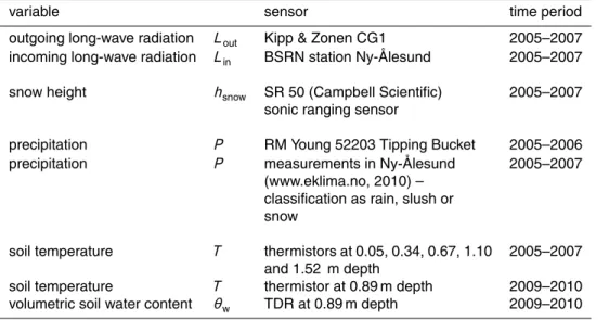
and the soil texture ranges from clay to silty loam (Boike et al., 2008). For this study, we use time series of outgoing long-wave radiation, from which the temperature of the ground or snow surface is calculated (Sect. 3.3). Furthermore, snow depth, ac-tive layer temperatures and soil water contents through “Time-Domain-Reflectometry” (TDR) measurements (Roth et al., 1990) within the active layer (Table 1) are employed. 10

As a record of GST, the soil temperature at 0.05 m depth below the surface in a de-pression between mudboils is used. The precipitation record from an unheated tipping bucket rain gauge, which only measures precipitation in the form of rain or slush, is em-ployed to determine the occurrence of rain-on-snow events and to coarsely estimate the amount of rain.

15

In addition, we make use of measurements of the incoming longwave radiation at a station of the “Baseline Surface Radiation Network” (BSRN) located in the village of Ny- ˚Alesund (Ohmura et al., 1998). Furthermore, precipitation measurements from Ny- ˚Alesund (www.eklima.no, 2010) are employed, where regular maintenance of the instrumentation is guaranteed, unlike at the Bayelva station. Here, the total amount 20

of precipitation is measured and the daily record is filed in the three classes “rain”, “slush” and “snow” according to visual observations, which allows an independent de-termination of rain-on-snow events. However, the exact amount of liquid precipitation cannot be determined from either record, as the partitioning of slush in liquid and solid precipitation is unclear.

(6)

TCD

5, 1697–1736, 2011

Title Page

Tables Figures

◭ ◮

Back Close

Full Screen / Esc

Discussion

P

a

per

|

Dis

cussion

P

a

per

|

Discussion

P

a

per

|

Discussio

n

P

a

per

|

3 Model setup

3.1 Soil thermal model

In the soil domain, we assume the temperatureT to change over time t and depthz

through heat conduction as described by

c_e_ff(z,T)∂T

∂t− ∂ ∂z

k(z,T)∂T

∂z

=0, (1)

5

where k(z,T) denotes the thermal conductivity and c_eff the effective heat capacity, which accounts for the latent heat of freezing and melting of water/ice as

c_eff=c(T,z)+L∂θw

∂T . (2)

L=334 MJ m−3denotes the specific volumetric latent heat of fusion of water. The first term is calculated from the volumetric fractions of the constituents as

10

c(T,z)₌X α

θα(T,z)cα, (3)

whereθα andcαrepresent the volumetric content and the specific volumetric heat ca-pacity (following Hillel, 1982) of the constituents water, ice, air, mineral and organic,

α=w,i,a,m,o. For the uppermost 10 m of soil, constant volumetric fractions of all con-stituents and heat capacities as given in Table 2 are employed, which are in agreement 15

with published values for the study site (Roth and Boike, 2001; Boike et al., 2008; West-ermann et al., 2009). The resulting volumetric heat capacities for frozen and unfrozen soil are given in Table 2. The soil freezing characteristicθ_w(T) is determined by fitting the function

θ_w(T)=

  

θwmin−(θwmax−θminw )Tδ−δ for T≤0 ◦

C

θ_wmax for T >0◦C

(7)

TCD

5, 1697–1736, 2011

Title Page

Tables Figures

◭ ◮

Back Close

Full Screen / Esc

Discussion

P

a

per

|

Dis

cussion

P

a

per

|

Discussion

P

a

per

|

Discussio

n

P

a

per

|

to measurements of temperature and soil water content conducted at a depth of 0.89 m (Table 1), which is displayed in Fig. 2. The fit yields a value ofδ=0.17◦C, and a resid-ual liquid water content in frozen soil ofθminw =0.05 is assumed (see Roth and Boike

(2001) for a discussion of the accuracy of TDR measurements in this context). The ice content is then given by

5

θi(T)=θwmax−θw(T). (5)

The thermal conductivityk is calculated following de Vries (1952) and Campbell et al. (1994) as

k=

P

αfαθαkα

P

αfαθα

, (6)

wheref_αdenotes a weighting factor andk_αthe conductivities of the constituents water, 10

ice, air and mineral (Hillel, 1982). The calculation of thef_αis guided by the concept that one of the constituents occurs as interconnected “continuous phase” with thermal con-ductivityk_c, while the other constituents are conceptualized as discontinuous phases, i.e. small domains intercepted by the continuous phase. Assuming spherical particles, the weighting factors can be calculated as (Campbell et al., 1994)

15

fα=

1₊1 3

_k

α

kc −1

−1

, (7)

wherek_cdenotes the conductivity of the continuous phase. For unfrozen soil with fixed mineral, but varying water and air contents, Campbell et al. (1994) suggest a smooth transition from an air-dominated regime (k_c=k_a) to a water-dominated regime (k_c=k_w) by defining

20

k_c=k_a+γ(k_w−k_a) (8)

with

γ=

1₊

_θ

w θ₀

−ǫs−1

(8)

TCD

5, 1697–1736, 2011

Title Page

Tables Figures

◭ ◮

Back Close

Full Screen / Esc

Discussion

P

a

per

|

Dis

cussion

P

a

per

|

Discussion

P

a

per

|

Discussio

n

P

a

per

|

The transition between air and water as continuous phase occurs at the “liquid recircu-lation cutoff”θ0, and the range, over which this transition takes place, is determined by

the smoothing parameterǫ_s. Campbell et al. (1994) give values for both parameters for a range of soils that have been determined in laboratory experiments. We employ values of θ0=0.1 and ǫs=3, which is in the range of the values found by Campbell

5

et al. (1994) for silty and clayey soils (as found in the study area).

We assume that the concept of Eq. (8) is applicable for air-ice systems (i.e. zero water content) and water-ice systems (i.e. zero air content). In the absence of mea-surements or literature values, we employ the same parametersθ₀andǫ_sfor the air-ice system as for the air-water system. For the water-ice system, the choice ofγ is un-10

critical, as the thermal conductivities of pure water and ice are not strongly different. We assume a linear interpolation betweenk_wandk_iaccording to the volumetric water and ice contents. Finally, the thermal conductivity of a soil with non-zero fractions of all constituents is obtained by interpolating between the three confining systems air-water, air-ice and water-ice, which span a three-dimensional space.

15

The resulting thermal conductivity for unfrozen soil isk_thawed=1.45 Wm−1K−1, which is in good agreement with the published value of (1.3±0.4) Wm−1K−1from

measure-ments in the study area (Westermann et al., 2009). For freezing soil in the temper-ature range between −2 and −9◦C at the Bayelva station, Roth and Boike (2001) report a thermal diffusivity of k/c_e_ff=8×10−7m2s−1. From the slope of the

freez-20

ing characteristic (Fig. 2), the volumetric fractions of all constituents and Eq. (3), c_eff

is estimated to be between 2.5 and 3.0 MJ m−3K−1 for this temperature range. This results in thermal conductivities between 2.0 and 2.4 Wm−1K−1, so that the value of

k_frozen=2.5 Wm−1K−1 obtained from the conductivity model for fully frozen soil is rea-sonable.

25

(9)

TCD

5, 1697–1736, 2011

Title Page

Tables Figures

◭ ◮

Back Close

Full Screen / Esc

Discussion

P

a

per

|

Dis

cussion

P

a

per

|

Discussion

P

a

per

|

Discussio

n

P

a

per

|

3.2 Snow thermal and hydrological model

If no liquid precipitation occurs, we assume heat transfer within the snow pack to be fully governed by conductive heat transfer. In case of a rain event, water freezes within the snow pack, which increases the volumetric ice contentθ_iand releases latent heat, thus increasing the snow temperatures towards the freezing point of water, 0◦C. The 5

governing equation of heat transfer within the snow pack thus becomes

c_snow∂T ∂t −

∂ ∂z

k_snow∂T ∂z

−L∂θi

∂t =0. (10)

For the densityρand the volumetric heat capacity of snow, we use published values from measurements of Westermann et al. (2009) at the study site (Table 3). To avoid inconsistencies due to mechanical e_ffects during freezing of water, the density of ice is 10

set equal to the density of water, so that a snow density of 350 kg m−3 _{corresponds to}

a volumetric ice content ofθ_i=0.35. For simplicity, we choose thermal conductivities which linearly increase from the date of the snowfall for each grid cell. The confining conductivitiesk_freshandk_old(Table 3) for fresh snow and for 280 days old snow (approx-imately corresponding to the length of the snow-covered period) are again derived from 15

Westermann et al. (2009): while the snow density and thus the volumetric heat capac-ity are found to be relatively homogeneous in time and space, an increase of measured thermal diffusivitiesk_snow/c_snowat the bottom of the snow pack from 4.5×10−7m2s−1 to 7.0×10−7m2s−1 is recorded from December to March. This corresponds to an

in-crease in thermal conductivity from 0.3 to 0.55 Wm−1_K−1_{, so that the chosen thermal}

20

conductivities are a good representation.

Infiltration of rain water is described by an extended bucket scheme, which distributes the liquid precipitation rate_∆P/∆tover the snow pack. In addition to temperature, two further variables are used to characterize a grid cell in each time step, the volumetric water contentθwand the sum of volumetric ice and water contents,θtot=θw+θi. For

25

(10)

TCD

5, 1697–1736, 2011

Title Page

Tables Figures

◭ ◮

Back Close

Full Screen / Esc

Discussion

P

a

per

|

Dis

cussion

P

a

per

|

Discussion

P

a

per

|

Discussio

n

P

a

per

|

– Isnow[s−1_{], leading to the infiltration of an amount of water, which refreezes and}

provides the energy to raise the temperature to 0◦C, plus infiltration establishing a maximum volumetric water content θfc_w, corresponding to the field capacity of the snow;

– Ibottom[s−1_{], which allows infiltration until the sum of ice and water content is unity,}

5

i.eθ_tot=1.

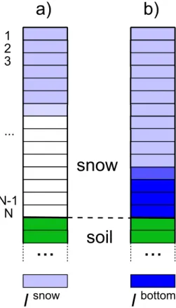
The scheme is schematically depicted in Fig. 3, details on the employed equations are given in Appendix A. The precipitation rate is distributed from top to bottom usingIsnow

for each grid cell, until the entire precipitation rate is accounted for (Fig. 3a). When the sum over the entire snow pack ofIsnowis not sufficient to absorb the precipitation rate, 10

water starts pooling at the bottom of the snow pack, which is treated by distributing

Ibottom from bottom to top (Fig. 3b) in the model. After the refreezing of this water, a bottom ice layer with thermal properties different from the snow forms (Table 3), for which literature values for ice are assigned (Hillel, 1982). Other than that, the thermal properties of the snow remain unchanged during and after an infiltration event.

15

Since both the exact amount of rain and the field capacityθ_wfccan only be estimated, we use a fixed value of 0.01 for the field capacity and manually adjust the solid-to-liquid ratio of the precipitation to fit the modeled GST to the measurements. For 2005/2006, we assume that 60 % of the daily precipitation recorded at the Bayelva station (which measures rain and slush) occur in liquid form. In 2006/2007, where only precipitation 20

data from Ny- ˚Alesund are available, only a single strong rain event occurs in late March. For this event, we consider the recorded precipitation as rain.

3.3 Time integration

The method of lines (Schiesser, 1991) is employed to numerically solve the heat transfer equation (Eq. 1) for a soil domain with 100 m depth. The spatial derivatives 25

(11)

TCD

5, 1697–1736, 2011

Title Page

Tables Figures

◭ ◮

Back Close

Full Screen / Esc

Discussion

P

a

per

|

Dis

cussion

P

a

per

|

Discussion

P

a

per

|

Discussio

n

P

a

per

|

resulting system of ordinary differential equations (ODE) is solved numerically in MAT-LAB with the ODE-solver “ode113” (Shampine and Gordon, 1975; Shampine and Re-ichelt, 1997), which continuously adjusts the integration time step to minimize compu-tational costs. The grid spacing is increased with depth, with 0.02 m between the sur-face (defined as 0 m) and 1.6 m, 0.2 m between 1.6 m and 5.0 m, 0.5 m between 5.0 m 5

and 20.0 m, 1.0 m between 20.0 m and 30.0 m, 5.0 m between 30.0 m and 50.0 m and 10.0 m between 50.0 m and 100.0 m.

If snow is present, additional grid cells with a grid spacing of 0.02 m are added on top of the soil. The position of the uppermost cell is determined from measurements of the snow depth, which are interpolated to the center positions of the snow grid cells. Within 10

the snow pack, the numerical scheme is applied to the variables (T θ_totθ_w), which are defined by the system of coupled differential equations given by Eq. (10), Eqs. (A4) to (A8) and Eq. (A9).

As upper boundary condition, we use surface temperatures T_surf based on mea-surements of outgoing and incoming long-wave radiation. For calculation, we use use 15

Stefan-Boltzmann and Kirchhoff’s Law,

L_out=εsσSTsurf4 +(1−εs)Lin, (11)

whereσ_S denotes the Stefan-Boltzmann constant and εs the surface emissivity. As this study focuses on periods, where the ground is snow-covered, we use a constant surface emissivity of 0.985, which is in the range of typical values published for snow 20

surfaces (e.g., Dozier and Warren, 1982; Hori et al., 2006). At the lower boundary, we prescribe a heat flux of 60 mW m−2 at a depth of 100 m, which is in the range of estimates for the geothermal heat flux on Svalbard (Liestøl, 1977; Isaksen et al., 2000; Van De Wal et al., 2002).

The initial condition is inferred from soil temperature measurements at the Bayelva 25

(12)

TCD

5, 1697–1736, 2011

Title Page

Tables Figures

◭ ◮

Back Close

Full Screen / Esc

Discussion

P

a

per

|

Dis

cussion

P

a

per

|

Discussion

P

a

per

|

Discussio

n

P

a

per

|

−3.9◦C, which is the average temperature of the temperature sensor at 1.52 m (which

has been continuously in frozen ground) for the period July 2002 to July 2005. At a depth of 100 m, the temperature is set to 0◦C, which is in agreement with estimates of permafrost thickness in coastal areas of Svalbard (Humlum, 2005).

If the snow depth increases and a new grid cell must be added from one time step 5

to the next, the temperature of the newly added grid cell, T₊, must be specified (for decreasing snow depths, the uppermost grid cell is simply deleted). We use

∂T₊

∂t =

T_surf(t)−T₊

τ₊ (12)

as defining differential equation, so thatT₊ follows the upper boundary condition with a characteristic lag timeτ₊. We set

10

τ₊=csnow(∆z) 2

k_snow , (13)

corresponding to the timescale of heat di_ffusion through snow over a distance_∆z (set to the grid spacing of 0.02 m). This choice ensures that the integration timesteps se-lected by the ode-solver are adequate both for the snow temperatures and forT₊. The volumetric ice and water content θ_tot of a snow cell is initialized to 0.35 according to 15

snow density measurements (Table 3, Westermann et al., 2009), while the water con-tentθ_wis set to zero.

4 Results

4.1 Field data from the winter seasons 2005/2006 and 2006/2007

We investigate the winter seasons 2005/2006 and 2006/2007, which are characterized 20

(13)

TCD

5, 1697–1736, 2011

Title Page

Tables Figures

◭ ◮

Back Close

Full Screen / Esc

Discussion

P

a

per

|

Dis

cussion

P

a

per

|

Discussion

P

a

per

|

Discussio

n

P

a

per

|

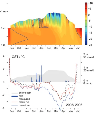
the course of September and lasts well into June of the following year. In 2005/2006, the snow depth is between 0.5 and 1.0 m for most of the winter period (Fig. 4). At the rain gauge at the Bayelva station, a total precipitation of 250 mm is recorded during the period when snow is present. At the same time, a total precipitation of 373 mm is measured in the village of Ny- ˚Alesund, of which 40 % are classified as snow, 47 % as 5

slush and 13 % as rain. As strong differences in the precipitation between the two sites are not likely, these numbers suggest that the 250 mm measured at the Bayelva station contain a considerable fraction of solid precipitation. Therefore, the total amount of liquid precipitation can only be estimated within wide margins of error from the mea-surements.

10

The measurements at the Bayelva station yield an average surface temperature of

−8.4◦C for the winter season of 2005/2006. The measured GST under the snow, how-ever, is much warmer and does not fall significantly below−1◦C for most of the winter

season. In December and January, rain events occur, after which the GST is con-fined to close to 0◦

C for several weeks. About 175 mm of precipitation are recorded 15

in Ny- ˚Alesund in this period, of which 40 mm are classified as rain and most of the remaining part as slush. At five days, the total measured precipitation exceeds 10 mm. In February, a stronger soil cooling is initiated: the minimum GST value of about−3◦C

is reached in the end of March after a prolonged period with snow surface tempera-tures as low as−25◦C, before the temperature increases again in the course of spring

20

(Fig. 4). The average GST during the period when the ground is covered by snow is

−0.6◦C.

In the winter period of 2006/2007, the measured snow depth is slightly higher than in the previous season, with values between 0.7 and 1.1 m for most of the winter. Due to problems with the rain gauge at the Bayelva station in this winter, only the precip-25

(14)

TCD

5, 1697–1736, 2011

Title Page

Tables Figures

◭ ◮

Back Close

Full Screen / Esc

Discussion

P

a

per

|

Dis

cussion

P

a

per

|

Discussion

P

a

per

|

Discussio

n

P

a

per

|

a sharp increase of the measured GST towards 0◦C (Fig. 5), to where the temperature is confined for about ten days. The average measured GST during the period, when the ground is covered by snow, is−1.1◦C, while the average snow surface temperature

is−9.8◦C.

From the yearly record of GST, the freezing and thawing indices, Fr and Th, are 5

calculated as the accumulated sum of degree days for negative and positive values of GST. Using the thermal conductivity for frozen and thawed soil (Table 2), we can evaluate a simple criterion for permafrost occurrence, (e.g., Carlson, 1952)

k_frozenFr, > k_thawedTh. (14)

For the period from July 2005 to June 2006, this condition is clearly violated, with 10

k_thawedTh being about twice as large as k_frozenFr. For the following year, both terms are approximately equal. The weighting might be even more shifted towards the right side of Eq. (14), since the soil is not fully frozen during part of the winter, so that the average thermal conductivity is smaller than k_frozen. In any case, the threshold, below which permafrost is sustainable on long timescales, is clearly exceeded for the 15

environmental conditions encountered in the winter season 2005/2006.

4.2 Model results

The strong di_fferences between the snow surface and the ground surface temperature encountered in both winter seasons form as a combination of two factors. First, the thermal insulation of the snow, which has a much lower thermal conductivity than the 20

underlying soil, delays the refreezing of the active layer, so that GST is sustained at higher values. Second, wintertime rain events cause a considerable warming of the snow and soil and can sustain GST at values close to 0◦C for prolonged periods. To separate both e_ffects, we use the permafrost model described in Sect. 3, which can simulate the thermal effect of rainwater infiltration on the soil. In addition to the model 25

(15)

TCD

5, 1697–1736, 2011

Title Page

Tables Figures

◭ ◮

Back Close

Full Screen / Esc

Discussion

P

a

per

|

Dis

cussion

P

a

per

|

Discussion

P

a

per

|

Discussio

n

P

a

per

|

Figure 4 depicts the modeled temperature distribution within the snow pack and the uppermost meter of the soil. In addition, the modeled ground surface temperatures (taken as the temperature at 0.05 m depth, see Sect. 2) from both the model and the control run are displayed. At the beginning of the season, the model slightly underesti-mates GST. A possible explanation is that the snow depth at the measurement location 5

in the depression between mudboils is higher than inferred from measurements with the sonic ranging sensor (Table 1), which averages over a larger footprint area. The impact of infiltrating rain is reflected in the position of the −0.01◦C isotherm (chosen

since the modeled temperatures never reach exactly 0◦C for computational reasons): after a rain event, the snow temperatures close to the surface rapidly cool, while the 10

temperatures in deeper snow layers remain around 0◦C, until all water is frozen. Dur-ing that time, the heat transfer to the snow surface is impeded by the overlyDur-ing snow layers, so that the freezing of the infiltrated water in the snow occurs slowly. If the infil-tration is sufficiently strong that water pools at the bottom of the snow pack and large quantities of water are stored in the bottom snow layers (due to the maximum infiltration 15

rateI_bottom, see Fig. 3b), the effect is particularly pronounced and confines the mod-eled GST to close to 0◦C for a prolonged period. This situation occurs in January and February 2006, where the model run reproduces the measured GST with reasonable accuracy, while the control run shows considerably cold-biased temperatures (Fig. 4), which persist for the rest of the winter season. In contrast, the rain events between 20

September and December 2005 have only minor impact on the modeled GST, so that the results of the model and the control run do not deviate strongly. As a result of the strong rain events, a 0.1 m thick bottom ice layer forms. Ice layers of similar thickness are documented for the area around Ny- ˚Alesund (Kohler and Aanes, 2004). The model run yields an average GST of−0.8◦C for the period, when the ground is covered by

25

snow, which is close to the measured value of −0.6◦C. The modeled average GST

in the control run is −1.5◦C, which still appears to be a good approximation of the

(16)

TCD

5, 1697–1736, 2011

Title Page

Tables Figures

◭ ◮

Back Close

Full Screen / Esc

Discussion

P

a

per

|

Dis

cussion

P

a

per

|

Discussion

P

a

per

|

Discussio

n

P

a

per

|

model run. Therefore, the permafrost is not sustainable according to Eq. (14) in the model run, while the control run suggests that the left and right side of Eq. (14) are approximately equal.

In the winter season 2006/2007, the GST obtained from model and control run do not deviate until March, despite of a few small rain events (Fig. 5). The impact of the 5

strong rain event in late March on GST is well reproduced in the model run, while the control run again yields cold-biased values of GST. Compared to the previous winter, the deviation between model and control run is smaller, with an average GST of−1.6◦C

in the control and−1.3◦C in the model run, compared to a measured average GST of −1.1◦C. The rain event results in the formation of a 0.04 m thick bottom ice layer. 10

In both seasons, the modeled GST is considerably colder than the measured GST at the end of the winter period, from end of April in 2006 and from mid of May in 2007 (Figs. 4 and 5). The step-like increase of measured GST is most likely caused by infiltration of water from melting snow, which is not accounted for in the current scheme. During this period, the agreement could most likely be improved, if near-surface melt 15

rates are calculated from a surface energy balance scheme (Boike et al., 2003). The infiltration of the melt water could then be treated similar to rain water.

4.3 Long-term impact of repeated winter rain events on the ground

thermal regime

It is evident from the measured freezing and thawing indices, that the permafrost at the 20

study site is not sustainable for the environmental conditions encountered in the winter season 2005/2006 (Sect. 4.1). To investigate the speed of a potential degradation and assess the contribution of the wintertime rain events, we force the model with the data set from July 2005 to June 2006 for ten consecutive years. As initial condition, we again prescribe the soil temperature distribution of 1 July 2005, as detailed in Sect. 3.3. We 25

emphasize, that the permafrost temperatures are comparatively low at this time, with an estimated temperature of−3.9◦C at 10 m depth. As the shape of the soil freezing

(17)

TCD

5, 1697–1736, 2011

Title Page

Tables Figures

◭ ◮

Back Close

Full Screen / Esc

Discussion

P

a

per

|

Dis

cussion

P

a

per

|

Discussion

P

a

per

|

Discussio

n

P

a

per

|

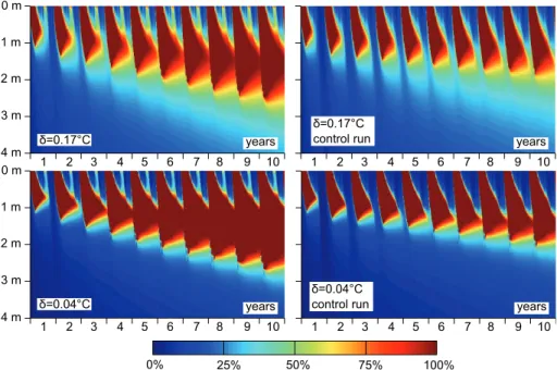
Osterkamp, 2000), we perform the simulation for two different parametersδ determin-ing the amount of unfrozen water at subzero temperatures. On the one hand, we use

δ=0.17◦C, as estimated for the silty to clayey soil at the Bayelva station (Fig. 2) and employed for the simulations in the previous section. On the other hand, the simulation is performed for a steeper soil freezing characteristic (δ=0.04◦C), which corresponds 5

to a soil of a higher sand and gravel content.

The results of the model and the control runs are displayed in Fig. 6, which shows the fraction of unfrozen soil water relative to the potentially freezable amount, i.e. θ_w/(θ_wmax−θmin_w ), for the uppermost four meters of the soil. While a zone with a considerable fraction of unfrozen soil water develops in all simulations, the degrada-10

tion occurs considerably faster for the model run, which includes the e_ffect of rain water infiltration, compared to the control run. For the flat soil freezing characteristic, the fi-nal temperature and soil water distribution of the control run after ten years is reached after roughly four years in the model run. Simultaneously, the maximum thaw depth increases by more than half a meter within three to four years in the model run, while 15

the increase is slower in the control run. For the steep soil freezing characteristic, the speed of degradation is even higher, with a zone with constantly unfrozen soil water forming after only three to four years in the model run, which after five years already extends over more than half a meter of soil. Again, the process is slower in the control run, although a zone with constantly unfrozen soil water develops at the end of the 20

ten-year period.

Sandy and gravelly areas, which most likely feature a steeper freezing characteristic, exist in the vicinity of the Bayelva station. A study by Westermann et al. (2010) demon-strates thaw depths of up to two meters in 2008 for a gravel plain located approximately 200 m from the Bayelva station, which might at least partly be a consequence of the 25

(18)

TCD

5, 1697–1736, 2011

Title Page

Tables Figures

◭ ◮

Back Close

Full Screen / Esc

Discussion

P

a

per

|

Dis

cussion

P

a

per

|

Discussion

P

a

per

|

Discussio

n

P

a

per

|

5 Discussion

5.1 Modeling wintertime rain events – challenges and improvements

The presented scheme makes use of a simplified bucket model of water infiltration in the snow, instead of solving the governing physical equations (e.g., Colbeck, 1972, 1979; Illangasekare et al., 1990). Nevertheless, it incorporates two important physical 5

constraints:

– Before water infiltration beyond a snow layer is possible, the temperature of the layer must be raised to 0◦C through freezing of the corresponding amount of water.

– A certain water content must be established and maintained to increase the hy-10

draulic permeability of the snow to a level that facilitates flow of water.

In the employed model, the two constraints are satisfied by choosing sufficiently small values for the parametersτ₁ andτ₂ (Eqs. A1 and A2), which control the timescales of the temperature increase to 0◦C and the saturation to the field capacity within a grid cell. We employ values on the order of seconds, so that (at least for realistic precip-15

itation rates) significant infiltration in a grid cell can only occur when both conditions are satisfied for the grid cell above. Therefore, the model produces a progressing wet-ting front in the snow, which is fundamental for correctly describing water infiltration in dry snow (Colbeck, 1976). In addition to the precipitation rate, the progression of the wetting front depends on the temperature and one free parameter, the field capac-20

ity θ_wfc of the snow, which can be adjusted to control the infiltration dynamics in dry snow. The physical interpretation of θwfc is the water content, at which the hydraulic

permeability switches from a very small value, which essentially prevents a flow, to a very large value, where flow is unobstructed and water movement occurs instantly. Accordingly, a precipitation signal instantly contributes to the water pool at the bottom 25

(19)

TCD

5, 1697–1736, 2011

Title Page

Tables Figures

◭ ◮

Back Close

Full Screen / Esc

Discussion

P

a

per

|

Dis

cussion

P

a

per

|

Discussion

P

a

per

|

Discussio

n

P

a

per

|

the snow is “wet”). In this point, the employed model differs from more sophisticated approaches describing the delay and dispersion of a precipitation pulse in wet snow by a hydraulic equation (e.g., Conway and Benedict, 1994). While the infiltration dynamics is not reproduced, the employed model still allows a good approximation of the amount of water reaching the bottom of the snow pack, which is the relevant quantity for the 5

thermal regime of the soil. Furthermore, the timescale of infiltration in wet snow is on the order of minutes to hours (e.g., Singh et al., 1997), while water can persist at the bottom of the snow pack for several weeks (Sect. 4.1), so that the infiltration dynamics is of minor relevance for the thermal regime of the permafrost.

In the model, we use a constant of value ofθ_wfc=0.01, independent of snow proper-10

ties, which is at the lower end of observed field capacities (denoted water holding ca-pacities in some studies). While Conway and Benedict (1994) and Singh et al. (1997) report field capacities of more than 0.05, Kattelmann (1986) outlines that field capac-ities of less than 0.02 are common. Furthermore, water infiltration in snow features a high degree of spatial variability, as it preferentially occurs along localized flow finger 15

(Conway and Raymond, 1993) or through fissures in ice layers in the snow pack, so that a spatially averaged value like θ_wfc (as employed in a 1-D-model) could be lower than suggested by measurements within a preferential flow path.

As exact rates of liquid precipitation are not available in this study, we cannot inde-pendently determineθwfc by fitting the model output to observed GST values, so that

20

it remains unclear whether the use of a constant value is su_fficient for the purpose of modeling the thermal regime of permafrost. However, more sophisticated modeling schemes that take into account a possible dependence of infiltration on snow prop-erties (e.g., Colbeck, 1979) generally require specification of additional parameters, for which a comprehensive set of field measurements is not available. Therefore, it 25

(20)

TCD

5, 1697–1736, 2011

Title Page

Tables Figures

◭ ◮

Back Close

Full Screen / Esc

Discussion

P

a

per

|

Dis

cussion

P

a

per

|

Discussion

P

a

per

|

Discussio

n

P

a

per

|

5.2 Impact assessment under different environmental conditions

The model runs presented in Sect. 3 illustrate that rain events only have a strong im-pact the soil temperatures, if water percolates to the bottom of the snow pack. This occurs if the amount of rain exceeds a threshold related to both temperature and water holding capacity of the snow. The energy required to cause an increase of the tem-5

perature of a snow pack of 1 m depth with the thermal properties given in Table 3 by 1 K corresponds to the latent heat released by the freezing of about 2.3 mm of water. Furthermore, for a field capacity of 0.01 as assumed in the model runs, 10 mm of wa-ter can be stored in the snow pack. For an average snow temperature of −5◦C, the threshold of liquid precipitation can thus be estimated to about 20 mm, which is only 10

exceeded by few rain events in the two investigated winter seasons. After rain water has percolated to the bottom of the snow pack, the freezing rate is controlled by the heat flux through the snow pack. For a constant snow surface temperature of−10◦C,

a snow depth of 1 m and a thermal conductivity of 0.5 Wm−1K−1, a heat flux of 5 Wm−2 is sustained, so that 10 mm of water at the bottom of the snow pack would freeze within 15

eight days. For a snow depth of 0.5 m, the freezing would occur within four days. In reality, the freezing would occur faster since a part of the latent heat contributes to the warming of the underlying soil, which subsequently cools via heat conduction through the snow.

Although large snow depths increase the threshold that must be exceeded for water 20

to reach the bottom of the snow pack, they also delay the freezing of the infiltrated water and thus increase the impact on soil temperatures. Therefore, rain events have the strongest impact on the soil temperatures if the snow depth is high and large amounts of rain fall within short periods, as it has been the case for the two events in January 2006 and March 2007. Furthermore, if repeated rain events occur within short periods 25

(21)

TCD

5, 1697–1736, 2011

Title Page

Tables Figures

◭ ◮

Back Close

Full Screen / Esc

Discussion

P

a

per

|

Dis

cussion

P

a

per

|

Discussion

P

a

per

|

Discussio

n

P

a

per

|

5.3 Accelerated permafrost degradation through wintertime rain events?

The multi-annual simulations presented in Sect. 4.3 suggest that rain-on-snow events can significantly accelerate the warming of soil temperatures in permafrost areas. As the long-term climate change is superimposed by considerable climate variability on shorter timescales, such non-linear processes can modify the response to the long-5

term warming signal: the occurrence of wintertime rain events may amplify the warm-ing of permafrost temperatures in case of positive temperature anomalies, while only the much slower process of heat conduction leads to subsequent cooling in case of negative anomalies, thus resulting in a stronger net warming.

Furthermore the model results highlight the possibility, that an initially stable per-10

mafrost system can quickly enter a state of degradation if environmental conditions as encountered in the winter 2005/2006 persist for several consecutive years. Thus, climate and weather extremes leading to an increased frequency of wintertime rain events may increase the vulnerability of permafrost to climate change.

Wintertime rain events play a larger role in permafrost regions with a maritime cli-15

mate compared to continental areas, where they are only reported in spring (Grois-man et al., 2003). Thus, the described processes are especially relevant for Svalbard and for mountain permafrost areas in Northern Europe. In Iceland, winter rain events are common at almost all elevation levels, producing iso-thermal snow conditions (Et-zelm ¨uller et al., 2007) and even contributing to the partial or total melting of the snow 20

pack (Farbrot et al., 2007). In Norway, winter rain events seems common over the en-tire mountain area and have recently been recorded at elevations of more than 1600 m (Farbrot et al., 2011). Regional climate projection for Scandinavia indicate an increase of winter precipitation, but also an increase of precipitation intensity and air temperature for the mountain areas (e.g., Benestad, 2005; Beldring et al., 2008). This suggests that 25

(22)

TCD

5, 1697–1736, 2011

Title Page

Tables Figures

◭ ◮

Back Close

Full Screen / Esc

Discussion

P

a

per

|

Dis

cussion

P

a

per

|

Discussion

P

a

per

|

Discussio

n

P

a

per

|

Furthermore, the pronounced changes in the arctic and sub-arctic climate system projected for the next 100 years (Solomon et al., 2007) may lead to the occurrence of wintertime rain events in permafrost area, where they have not been recorded previ-ously or where such events have been very rare. Rennert et al. (2009) have scanned the output of GCMs for synoptic conditions correlated to the occurrence of winter rain 5

events. Their analysis suggests an increase of both the frequency and the areal extent over the next 50 years, with Northwestern Canada, Alaska, and the pacific regions of Siberia being among the most affected areas.

Wintertime rain events are not accounted for in the models used to predict the future extent and thermal regime of permafrost. This study suggests that incorporating the 10

effects of such events could improve predictions at least for regions where they oc-cur regularly. While the presented model could in principle be driven with precipitation data sets obtained from climate models, it is questionable whether such coarse-scale models can sufficiently capture the threshold nature of wintertime rain events. Fur-thermore, climate models deliver average precipitation rates for large grid cells, which 15

cannot reproduce a the subgrid variability typical for strong precipitation events. Due to the non-linearity of the rainwater infiltration in the snow, statistical (Wilby et al., 1998) or stochastic (Bates et al., 1998) downscaling algorithms may be required in order to correctly reproduce the net effect of wintertime rain events on long timescales.

6 Conclusions

20

We present measurements of the ground surface temperature conducted during two winter seasons on W Svalbard, where a number of wintertime rain events have oc-cured. A simplified model of rainwater infiltration coupled to a transient permafrost model is employed to separate the impact of the rain events on soil temperatures from the thermal effects of the insulating snow cover. From this study the following conclu-25

(23)

TCD

5, 1697–1736, 2011

Title Page

Tables Figures

◭ ◮

Back Close

Full Screen / Esc

Discussion

P

a

per

|

Dis

cussion

P

a

per

|

Discussion

P

a

per

|

Discussio

n

P

a

per

|

– Small amounts of rain freeze close to the snow surface and thus have negligible impact on the soil temperatures.

– Strong rain events can modify the ground surface temperature over prolonged periods. During such periods, a permafrost model based solely on conductive heat transfer cannot reproduce the measured ground surface temperatures and 5

rain water infiltration must be taken into account.

– In one of the investigated winter seasons, an average ground surface temperature of−0.6◦C is measured, despite of an average snow surface temperature below −8◦C. As a consequence, the temperature threshold, below which permafrost is

sustainable on long timescales, is clearly exceeded according to a simple degree-10

day model.

– In a model simulation, where the environmental conditions encountered in this winter are repeatedly applied for several consecutive winters, clear evidence of permafrost degradation is visible after three to five years, as a zone develops, where only a minor part of the soil water refreezes. In a control run, where rain 15

water infiltration is not accounted for, twice the time is required to reach a similar state.

– Strong wintertime rain events have a distinct impact on soil temperatures. As a process of highly non-linear nature, they have the potential to generate an ac-celerated warming in case of climate extremes, during which they occur with in-20

(24)

TCD

5, 1697–1736, 2011

Title Page

Tables Figures

◭ ◮

Back Close

Full Screen / Esc

Discussion

P

a

per

|

Dis

cussion

P

a

per

|

Discussion

P

a

per

|

Discussio

n

P

a

per

|

Appendix A

Governing equations of snow thermal and hydrological regime

The maximum infiltration rates (see Sect. 3.2) are given by

Isnow = csnow L

T_f−T

τ₁ −

1

L ∂ ∂z

ksnow ∂T ∂z

5

+θ fc w−θw

τ₂ (A1)

Ibottom = 1−θtot

τ₂ , (A2)

whereT_f is the freezing temperature of water (set to 0◦C). In the model runs, we use

τ1=τ2=10 s, so that the timescale of infiltration in a grid cell is short compared to

the timescale of conductive heat transfer. Ifθ_tot=θ_w+θ_i reaches one for a grid cell, 10

bothIsnowandIbottom are set to zero, thus preventing further infiltration. Note, that this condition is inherent in the definition ofIbottom, but not in Isnow. The derivative of θ_tot

with respect to time is calculated with a recursive scheme. The snow grid cells are indexed from top to bottom asj=1,...,N, withN being the grid cell above the snow-soil interface (Fig. 3). Using finite differences (see Sect. 3.3), Eqs. (A1) and (A2) are 15

discretized in space, yielding the infiltration ratesI_jsnowandI_jbottomfor each grid cell. For

∆P ∆t ≤

N

X

j=1

I_jsnow, (A3)

corresponding to the case depicted in Fig. 3 a, ∂θtot/∂t of the first and then-th grid

cell are calculated from top to bottom as

_∂θ

tot ∂t

1 =min

∆P ∆t,I

snow 1

(25)

TCD

5, 1697–1736, 2011

Title Page Abstract Introduction Conclusions References Tables Figures ◭ ◮ ◭ ◮ Back Close

Full Screen / Esc

Printer-friendly Version Interactive Discussion Discussion P a per | Dis cussion P a per | Discussion P a per | Discussio n P a per | _∂θ tot ∂t n =min  ∆ P ∆t −

n−1

X j=1 _∂θ tot ∂t j

,I_nsnow



. (A5)

If condition (A3) is not fulfilled, i.e. for the case depicted in Fig. 3 b,∂θtot/∂tof the N-th

andn-th grid cells are calculated from bottom to top as

_∂θ tot ∂t N =min   ∆P ∆t −

N−1

X

j=1

I_jsnow,I_Nbottom

  (A6) _∂θ tot ∂t n =min   ∆P ∆t −

n−1

X

j=1 I_jsnow−

N

X

j=n+1

_∂θ

tot ∂t

j

,I_nbottom



. (A7)

5

For simplicity, spatial derivatives instead of finite di_fferences are given in the following. The derivative of the volumetric water contentθ_wwith respect to time is calculated as

∂θ_w ∂t =            ∂θ_tot ∂t − c_snow L

Tf−T τ₁ +1 L ∂ ∂z

k_snow∂T ∂z

for θ_w>0

0 for θ_w=0

. (A8)

This yields the derivative of the ice contentθ_iwith respect to time as

∂θ_i

∂t =

∂θ_tot

∂t −

∂θ_w

∂t , (A9)

10

which is employed in Eq. (10), where this term describes the effect of refreezing water on the temperatures in the snow pack.

(26)

TCD

5, 1697–1736, 2011

Title Page

Tables Figures

◭ ◮

Back Close

Full Screen / Esc

Discussion

P

a

per

|

Dis

cussion

P

a

per

|

Discussion

P

a

per

|

Discussio

n

P

a

per

|

case the infiltration rate for a grid cell is equal to the maximum infiltration rate, i.e.

∂θ_tot/∂t= Isnow, the derivative of the ice content becomes

∂θ_i

∂t =

c_snow L

T_f−T

τ₁ −

1

L ∂ ∂z

ksnow ∂T ∂z

. (A10)

Equation (10) controlling the temperature evolution within the snow pack simplifies to

c_snow∂T

∂t =csnow T_f−T

τ₁ , (A11)

5

so that the temperature exponentially approachesT_fwith time constantτ₁as

T(t)=Tf+T(t0)e−t/τ1. (A12)

Similarly, the liquid water content exponentially saturates towards the field capacityθfc_w

with the governing differential equation

∂θw

∂t =

θwfc−θw

τ₂ . (A13)

10

In the following, the temperature is sustained at T_f, as the amount of freezing water balances the conductive heat flux to the neighboring grid cells, which is determined by the gradient of the heat flux, −∂/∂z(k_snow∂T/∂z). When the infiltration process ceases,∂θ_tot/∂tbecomes zero. For a grid cell withθ_w>0 andT=T_f, the water content decreases according to

15

∂θ_w

∂t =

1

L ∂ ∂z

k_snow∂T ∂z

≤0, (A14)

as heat is flowing out into neighboring colder grid cells. With∂θ_i/∂t=−∂θ_w/∂t, the

(27)

TCD

5, 1697–1736, 2011

Title Page

Tables Figures

◭ ◮

Back Close

Full Screen / Esc

Discussion

P

a

per

|

Dis

cussion

P

a

per

|

Discussion

P

a

per

|

Discussio

n

P

a

per

|

Acknowledgements. We are grateful to M. Maturilli for providing us with the data of the BSRN station used to correct the surface temperature record. We thank the personnel of the AWIPEV base in Ny- ˚Alesund for the ongoing support of our permafrost research, which contributed greatly to the success of this work.

References

5

Bartsch, A.: Ten years of SeaWinds on QuikSCAT for snow applications, Remote Sens., 2, 1142–1156, 2010. 1699

Bartsch, A., Kumpula, T., Forbes, B., and Stammler, F.: Detection of snow surface thawing and refreezing in the Eurasian Arctic using QuikSCAT: implications for reindeer herding, Ecol. Appl., 20(8), 2346-2358, doi:10.1890/09-1927, 2010. 1699

10

Bates, B., Charles, S., and Hughes, J.: Stochastic downscaling of numerical climate model simulations, Environ. Modell. Softw., 13, 325–331, 1998. 1718

Beldring, S., Engen-Skaugen, T., Førland, E., and Roald, L.: Climate change impacts on hydro-logical processes in Norway based on two methods for transferring regional climate model results to meteorological station sites, Tellus A, 60, 439–450, 2008. 1717

15

Benestad, R.: Climate change scenarios for Northern Europe from multi-model IPCC AR4 climate simulations, Geophys. Res. Lett, 32, L17704, doi:10.1029/2005GL023401, 2005. 1717

Boike, J., Roth, K., and Ippisch, O.: Seasonal snow cover on frozen ground: energy balance calculations of a permafrost site near Ny- ˚Alesund, Spitsbergen, J. Geophys. Res.-Atmos., 20

108, 8163–8173, 2003. 1700, 1712

Boike, J., Ippisch, O., Overduin, P., Hagedorn, B., and Roth, K.: Water, heat and solute dynam-ics of a mud boil, Spitsbergen, Geomorphology, 95, 61–73, 2008. 1700, 1701, 1702

Campbell, G., Jungbauer Jr, J., Bidlake, W., and Hungerford, R.: Predicting the effect of tem-perature on soil thermal conductivity, Soil Sci., 158, 307–313, 1994. 1703, 1704

25

Carlson, H.: Calculation of depth of thaw in frozen ground, Highway Research Board Special Report, 2, 192–223, Highway Research Board, Washington DC, USA, 1952. 1710

Chan, K., Mysterud, A., Øritsland, N., Severinsen, T., and Stenseth, N.: Continuous and dis-crete extreme climatic events affecting the dynamics of a high-arctic reindeer population, Oecologia, 145, 556–563, 2005. 1700

(28)

TCD

5, 1697–1736, 2011

Title Page

Tables Figures

◭ ◮

Back Close

Full Screen / Esc

Discussion

P

a

per

|

Dis

cussion

P

a

per

|

Discussion

P

a

per

|

Discussio

n

P

a

per

|

Colbeck, S.: A theory of water percolation in snow, J. Glaciol., 11, 369–385, 1972. 1714 Colbeck, S.: An analysis of water flow in dry snow, Water Resour. Res., 12, 523–527, 1976.

1714

Colbeck, S.: Water flow through heterogeneous snow, Cold Reg. Sci. Technol., 1, 37–45, 1979. 1714, 1715

5

Conway, H. and Benedict, R.: Infiltration of water into snow, Water Resour. Res., 30, 641–649, 1994. 1715

Conway, H. and Raymond, C.: Snow stability during rain, J. Glaciol., 39, 1993. 1715

Delisle, G.: Near-surface permafrost degradation: how severe during the 21st century?, Geo-phys. Res. Lett., 34, 9503, doi:10.1029/2007GL029323, 2007. 1698

10

Dozier, J. and Warren, S.: Effect of viewing angle on the infrared brightness temperature of snow, Water Resour. Res., 18, 1424–1434, 1982. 1707

Etzelm ¨uller, B., Farbrot, H., Guð_{mundsson, ´}_{A., Humlum, O., Tveito, O., and Bj ¨ornsson, H.: The}

regional distribution of mountain permafrost in Iceland, Permafrost Periglac., 18, 185–199, 2007. 1699, 1717

15

Etzelm ¨uller, B., Schuler, T. V., Isaksen, K., Christiansen, H. H., Farbrot, H., and Benestad, R.: Modeling the temperature evolution of Svalbard permafrost during the 20th and 21st century, The Cryosphere, 5, 67–79, doi:10.5194/tc-5-67-2011, 2011. 1699

Farbrot, H., Etzelm ¨uller, B., Schuler, T., Guð_{mundsson, ´}_{A., Eiken,} _{T., Humlum, O., and}

Bj ¨ornsson, H.: Thermal characteristics and impact of climate change on mountain per-20

mafrost in Iceland, J. Geophys. Res., 112, F03S90, doi:10.1029/2006JF000541, 2007. 1699, 1717

Farbrot, H., Etzelm ¨uller, B., Hipp, T., Isaksen, K., Ødeg ˚ard, R., Schuler, T., and Humlum, O.: Air and ground temperatures along elevation and continental gradients in Southern Norway, submitted to Permafrost Periglac., 2011. 1717

25

Førland, E. and Hanssen-Bauer, I.: Increased precipitation in the Norwegian Arctic: true or false?, Climatic Change, 46, 485–509, 2000. 1715

Førland, E., Hanssen-Bauer, I., and Nordli, P.: Climate statistics and longterm series of tem-peratures and precipitation at Svalbard and Jan Mayen, Det Norske Meteorologiske Institutt Klima Report 21/97, Oslo, Norway, 1997. 1700

30