www.geosci-model-dev.net/4/845/2011/ doi:10.5194/gmd-4-845-2011
© Author(s) 2011. CC Attribution 3.0 License.
Geoscientific
Model Development
MIROC-ESM 2010: model description and basic results of
CMIP5-20c3m experiments
S. Watanabe1, T. Hajima1, K. Sudo2, T. Nagashima3, T. Takemura4, H. Okajima1, T. Nozawa2,3, H. Kawase3, M. Abe3, T. Yokohata3, T. Ise1, H. Sato2, E. Kato1, K. Takata1, S. Emori1,3, and M. Kawamiya1
1Japan Agency for Marine-Earth Science and Technology, Yokohama, Japan 2Graduate School of Environmental Studies, Nagoya University, Nagoya, Japan 3National Institute for Environmental Studies, Tsukuba, Japan
4Research Institute for Applied Mechanics, Kyushu University, Kasuga, Japan Received: 25 April 2011 – Published in Geosci. Model Dev. Discuss.: 17 May 2011 Revised: 14 September 2011 – Accepted: 16 September 2011 – Published: 4 October 2011
Abstract. An earth system model (MIROC-ESM 2010) is fully described in terms of each model component and their interactions. Results for the CMIP5 (Coupled Model Inter-comparison Project phase 5) historical simulation are pre-sented to demonstrate the model’s performance from sev-eral perspectives: atmosphere, ocean, sea-ice, land-surface, ocean and terrestrial biogeochemistry, and atmospheric chemistry and aerosols. An atmospheric chemistry coupled version of MIROC-ESM (MIROC-ESM-CHEM 2010) rea-sonably reproduces transient variations in surface air tem-peratures for the period 1850–2005, as well as the present-day climatology for the zonal-mean zonal winds and tem-peratures from the surface to the mesosphere. The historical evolution and global distribution of column ozone and the amount of tropospheric aerosols are reasonably simulated in the model based on the Representative Concentration Path-ways’ (RCP) historical emissions of these precursors. The simulated distributions of the terrestrial and marine biogeo-chemistry parameters agree with recent observations, which is encouraging to use the model for future global change pro-jections.
1 Introduction
The establishment of long-term mitigation goals against cli-mate change should be based on sound information from sci-entific projections on a centennial time scale. Tools that have been developed for reliable projection include numerical cli-mate models (e.g. K-1 model developers, 2004), future sce-narios (Moss et al., 2010), and model experimental design
Correspondence to:S. Watanabe ([email protected])
(Hibbard et al., 2007; Meehl and Hibbard, 2007; Taylor et al., 2009). These efforts are mutually cooperative and ex-pected to enhance collaboration among different communi-ties working on model development, impact assessment and scenario development (Moss et al., 2010). Projections made up to year 2300 using this approach will aid the refinement of policies for greenhouse gas (GHG) reduction by, say, 2050 (Miyama and Kawamiya, 2009).
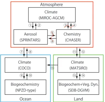
Atmosphere Climate (MIROC-AGCM) Aerosol (SPRINTARS) Chemistry (CHASER) Climate (COCO) Biogeochemistry (NPZD-type) Ocean Climate (MATSIRO) (SEIB-DGVM) Land Biogeochem+Veg. Dyn.
① ② ③ ④
⑤ ⑥ ⑦ ⑧ ⑨ ⑩ ⑪ ⑫ ⑬ ⑭ ⑮
Fig. 1. Structure of MIROC-ESM. The numbers refer to the vari-ables in Table 1.
In response to these issues, earth system models (ESMs), which is often used as a synonym for coupled climate models with biogeochemical components, are now being developed at leading institutes for climate science (e.g. Tjiputra et al., 2010; Weaver et al., 2001; Hill et al., 2004; Redler et al., 2010). This work describes the structure and performances of an ESM developed on the basis of the version presented by Kawamiya et al. (2005) at the Japan Agency for Marine-Earth Science and Technology (JAMSTEC) in collaboration with, among others, the University of Tokyo and the National Institute for Environmental Studies (NIES).
2 Model description
Our ESM, named “MIROC-ESM”, is based on a global cli-mate model MIROC (Model for Interdisciplinary Research on Climate) which has been cooperatively developed by the University of Tokyo, NIES, and JAMSTEC (K-1 model de-velopers, 2004; Nozawa et al., 2007). A comprehensive at-mospheric general circulation model (MIROC-AGCM 2010) including an on-line aerosol component (SPRINTARS 5.00), an ocean GCM with sea-ice component (COCO 3.4), and a land surface model (MATSIRO) are interactively coupled in MIROC as illustrated in Fig. 1. These atmosphere, ocean, and land surface components, as well as a river routing scheme, are coupled by a flux coupler (K-1 model develop-ers, 2004).
On the basis of MIROC, MIROC-ESM further includes an atmospheric chemistry component (CHASER 4.1), a nutrient-phytoplankton-zooplankton-detritus (NPZD) type
ocean ecosystem component, and a terrestrial ecosystem component dealing with dynamic vegetation (SEIB-DGVM). Table 1 shows the modeled variables that are exchanged among the components of MIROC-ESM, and the numbered arrows in Fig. 1 indicate the pathways of these variables.
Due to given large uncertainty in coupling processes, the present version of MIROC-ESM includes some limited pro-cesses, only: e.g. effects of vegetation changes on dust emis-sion, and effects of deposition of black carbon (BC) and dust on snow albedo (see Sect. 2.3.1). Many coupling processes, which are potentially important in the Earth system, are not included at present. For example: the atmospheric chem-istry and aerosols are not directly coupled with ecosystems at present. Biogenic emissions of dimethylsulfide (DMS) do not depend on the ocean biogeochemistry. Vegetation changes do not affect biogenic emissions of atmospheric compositions including ozone and aerosol precursors, though changes in biogenic volatile organic compounds (VOCs) due to land use change could be effective in the corresponding re-gions in the real world (Sudo et al., 2010). Ozone and other ecologically harmful gases and acids, and ultraviolet radia-tion do not damage ecosystems.
As a total integration period of many thousands of years was requested for the series of CMIP5 (Coupled Model In-tercomparison Project phase-5) experiments on long-term fu-ture climate projections (Taylor et al., 2009), the number of experiments that would be performed with the full version of MIROC-ESM had to be limited. Therefore, a limited number of experiments were performed using the CHASER-coupled version of MIROC-ESM (MIROC-ESM-CHEM), while all of the requested experiments were performed using a ver-sion without the coupled atmospheric chemistry, referred to as MIROC-ESM hereafter. In later literatures the present ver-sion of MIROC-ESM and MIROC-ESM-CHEM would be referred to with the year 2010 like “MIROC-ESM 2010”. By comparing results of these two versions, the importance of chemistry climate interactions on the transient climate sys-tem may be estimated, although this is beyond the scope of the present paper. Each component of MIROC-ESM-CHEM will be described in the following subsections.
2.1 Atmospheric model
2.1.1 MIROC-AGCM
Table 1. Variables exchanged between each model component.
Within Atmosphere
(1) Climate (MIROC-AGCM)⇒Aerosols (SPRINTARS)
Specific Humidity
Mass Mixing Ratio of Cloud (Water plus Ice) Mass Mixing Ratio of Aerosols (Each Component) Cloud Droplet Number Concentration
Ice Crystal Number Concentration Surface Air Pressure
Air Temperature Surface Altitude Land Area Fraction
Near-Surface Air Temperature Eastward Near-Surface Wind Speed Northward Near-Surface Wind Speed Diffusion Coefficient
Near-Surface Wind Speed due to Dry Convection Omega
Solar Zenith Angle Soil Moisture Snow Amount
Surface Downwelling Shortwave Radiation Sea Ice Concentration
Total Cloud Fraction Leaf Area Index Precipitation
Convective Cloud Area Fraction Stratiform Cloud Area Fraction
Mass Mixing Ratio of Cloud Liquid Water Mass Mixing Ratio of Cloud Ice Mass Fraction of Cloud Liquid Water
Tendency of Air Temperature due to Radiative Heating time
time step
(2) Aerosols (SPRINTARS)⇒Climate (MIROC-AGCM)
Specific Humidity
Mass Mixing Ratio of Cloud (Water plus Ice) Mass Mixing Ratio of Aerosols (Each Component) Cloud Droplet Number Concentration
Ice Crystal Number Concentration
Mass Mixing Ratio of Aerosols for Radiation Code
(3) Climate (MIROC-AGCM)⇒Chemistry (CHASER)
Air temperature (3-D & surface) Specific humidity
Relative humidity Eastward wind Northward wind Vertical wind Convective mass flux
cloud area fraction (3-D & surface) atmosphere cloud condensed water content atmosphere cloud ice content
Table 1.Continued.
convective precipitation flux
tendency of cloud condensed water content tendency of cloud ice content
subgrid diffusion coefficients upward shortwave flux (3-D & surface) downward shortwave flux (3-D & surface)
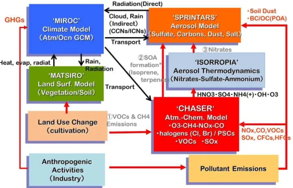
(4) Chemistry (CHASER)⇒Climate (MIROC-AGCM) specific humidity
mole fraction of O3in air
mole fraction of CH4in air
mole fraction of N2O in air
mole fraction of Halocarbons in air
(5) Aerosols (SPRINTARS)⇒Chemistry (CHASER) aerosol surface density in air
mole fraction of dust aerosol in air
(6) Chemistry (CHASER)⇒Aerosols (SPRINTARS) mole fraction of OH in air
mole fraction of O3in air
mole fraction of H2O2in air
#mole fraction & number density of SO4in air
#mole fraction & number density of aerosol nitrate in air #mole fraction & number density of SOA in air #aerosol water in air
#CHASER on-line aerosol simulation (not used in CMIP5 simulations) (7) Atmosphere⇒Ocean
Eastward Wind (lowest layer) Northward Wind (lowest layer) Air Temperature (lowest layer) Specific Humidity (lowest layer) Air Pressure
Surface Air Pressure Surface Height
Net Downward Shortwave Radiation at Sea Water Surface Solar Zenith Angle
Mole Fraction of CO2in Air
Henry constant (for CHASER)
precipitation flux: cumulus (for CHASER)
precipitation flux: Large Scale Condensation (for CHASER) latitude
(8) Ocean⇒Atmosphere Albedo
Surface Temperature Surface Upward CO2Flux
Bulk Coefficient Sea Ice Mass
deposition velocity for CHASER
biological emission flux (terpenes, isoprene) for CHASER (9) Ocean⇒Ocean biogeochemistry
Sea Water Potential Temperature
Net Downward Shortwave Radiation at Sea Water Surface Solar Zenith Angle
Surface Upward CO2Flux
Table 1.Continued.
Zooplankton Carbon Concentration Detrital Organic Carbon Concentration Calcite Concentration
Calcium
Dissolved Inorganic Carbon Concentration Total Alkalinity
Sea Water Salinity
(10) Ocean biogeochemistry⇒Ocean Surface Aqueous Partial Pressure of CO2
Sea Water CO2Solubility
(11) Atmosphere⇒Land (MATSIRO) Eastward Wind (lowest layer) Northward Wind (lowest layer) Air temperature (lowest layer) Specific humidity (lowest layer) Air pressure (Lowest layer/Surface)
Downward radiation fluxes (6 components: Visible/Near Infrared/Infrared, Direct/Diffuse) Solar Zenith Angle (for parameterization of radiation transfer in canopy)
Mole Fraction of CO2in Air (lowest layer)
Henry constant (from CHASER)
Precipitation (including snowfall, 2 types: cumulus/large-scale condensation) Surface deposition of soil dust (from SPRINTARS)
Surface deposition of black carbon (from SPRINTARS) (12) Land (MATSIRO) ->Atmosphere
Surface Upward Eastward Wind Stress Surface Upward Northward Wind Stress Surface Upward Sensible heat flux Surface Upward Latent heat flux
Upward radiation fluxes (Short wave/Long wave)
Albedo (6 components: Visible/Near Infrared/Infrared, Direct/Diffuse) Surface temperature
Evapotranspiration (6 components: Transpiration/Interception/Ground, Evaporation/Sublimation) Snow sublimation
10 m Wind (to SPRINTARS, CHASER) 2 m temperature (to SPRINTARS, CHASER) 2 m Specific humidity (to SPRINTARS, CHASER) Surface wetness (to SPRINTARS)
Snow water equivalent (to SPRINTARS) Bulk coefficient for eddy transfer (to SPRINTARS)
Deposition fluxes of tracers (lowerst layer/surface) (to CHASER) Emission (to CHASER)
(13) MATSIRO⇒SEIB-DGVM Precipitation
Downward short wave radiation Mole fraction of CO2in air
2 m temperature Eastward 10 m wind speed Northward 10 m wind speed 2 m Specific humidity Soil temperature
(14) SEIB-DGVM⇒MATSIRO Leaf Area Index
Atmosphere-Land carbon flux (Net carbon balance) (Through to Atmosphere) (15) MATSIRO ->Ocean
in the present study. Unlike other setups of the MIROC-AGCM, MIROC-ESM has the fully resolved stratosphere and mesosphere (Watanabe et al., 2008a). The hybrid terrain-following (sigma) pressure vertical coordinate system is used, and there are 80 vertical layers between the surface and about 0.003 hPa. In order to obtain the spontaneously generated equatorial quasi-biennial oscillation (QBO), a fine vertical resolution of about 680 m is used in the lower strato-sphere.
The MIROC-AGCM has a suite of physical parameteriza-tions that are detailed in K-1 model developers (2004) and Nozawa et al. (2007). Watanabe et al. (2008a) describes the modifications and inclusions of physical parameterizations from MIROC-AGCM to MIROC-ESM that are crucial for the representation of the large-scale dynamical and thermal structures in the stratosphere and mesosphere. A brief sum-mary of the physical parameterization is given in the follow-ing.
The radiative transfer scheme adopted in MIROC-ESM follows Sekiguchi and Nakajima (2008) and is an updated version of the k-distribution scheme used in the previous versions of MIROC-AGCM. Watanabe et al. (2008a) illus-trated the improvements of the simulated thermal structure in MIROC-ESM-CHEM by replacing the old scheme with the new one. The present scheme considers 29 and 37 ab-sorption bands in MIROC-ESM and MIROC-ESM-CHEM, respectively. The spectral resolution in visible and ultra vi-olet regions is increased from 15 in MIROC-ESM to 23 in MIROC-ESM-CHEM, because detailed calculations are re-quired for photolysis. Direct and indirect effects of aerosols are considered in the radiation scheme, which will be de-scribed in Sect. 2.1.2.
The cumulus parameterization is based on the scheme pre-sented by Arakawa and Schubert (1974). A prognostic clo-sure is used in the cumulus scheme, in which cloud base mass flux is treated as a prognostic variable. An empirical cumulus suppression condition is introduced (Emori et al., 2001), by which cumulus convection is suppressed when cloud mean ambient relative humidity is less than a critical value. This is a parameter by which the spatio-temporal distribution of the parameterized cumulus precipitation, and hence charac-teristics of vertically propagating atmospheric waves gener-ated by cumulus convection, are strongly controlled. In the present setup of MIROC-ESM, a value of 0.7 is used for this parameter to generate moderate convective precipitation and a moderate wave momentum flux associated with the re-solved atmospheric waves.
The large-scale (grid-scale) condensation is diagnosed based on the scheme of Le Treut and Li (1991) and a sim-ple cloud microphysics scheme. In MIROC-ESM, the cloud phase (solid or liquid) is diagnosed according to the temper-ature,T:
fliq=exp(−((Ts− −T )/Tf)2) (T > Tm), fliq=0 (T < Tm),
where fliq is the ratio of liquid cloud water to total cloud water, andTm,Ts, andTfare set to 235.15 K, 268.91 K, and 12.0 K, respectively.
The sub-grid vertical mixing of prognostic variables is calculated on the basis of the level 2 scheme of the turbu-lence closure model by Mellor and Yamada (1974, 1982). MIROC-ESM uses ∇6 horizontal hyper viscosity diffusion
to suppress the effect of extra energies at the largest hori-zontal wave number. The horihori-zontal diffusion is not applied to the tracers since the tracer advection scheme is separated from the spectral dynamical core of MIROC-AGCM. The e-folding time for the smallest resolved wave is 0.5 days. In order to prevent extra wave reflection at the top boundary, a sponge layer is added to the top level, which causes the wave motions to be greatly dampened.
The effects of orographically and non-orographically gen-erated subgrid-scale internal gravity waves are parameterized following McFarlane (1987) and Hines (1997), respectively (Watanabe et al., 2008a). As documented in Watanabe et al. (2008a) and Watanabe (2008), the present-day climatol-ogy of non-orographic gravity wave source spectra estimated using results of a gravity wave-resolving version of MIROC-AGCM (Watanabe et al., 2008b) are launched at 70 hPa in the extratropics of MIROC-ESM. The non-orographic grav-ity waves are mainly emitted from convection, jet-frontal sys-tems, and adjustment processes, in the troposphere, prop-agating upward to the 70 hPa level. In the tropics, an isotropic source of non-orographic gravity waves is launched at 650 hPa in the present version. The strength of the tropical source is arbitrarily tuned so that the QBO with a realistic period of 27–28 months on average can be reproduced under present-day (2000s) conditions. As a consequence, the pe-riod of simulated QBO elongates with increasing GHG con-centrations due to strengthening of the Brewer-Dobson cir-culation in the stratosphere (Watanabe and Kawatani, 2011). 2.1.2 Aerosol module – SPRINTARS
module. Number concentrations for cloud droplets and ice crystals are prognostic variables as well as their mass mixing ratios, and changes in their radii and precipitation rates are calculated for the indirect effect. More detailed descriptions of SPRINTARS can be found in Takemura et al. (2000) for the aerosol transport, Takemura et al. (2002) for the aerosol direct effect, and Takemura et al. (2005, 2009) for the aerosol indirect effect on water and ice clouds. Some improvements to each process are described in the later references. 2.1.3 Chemistry module – CHASER
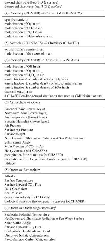
Simulations of atmospheric chemistry in MIROC-ESM-CHEM are based on the chemistry model CHASER (Sudo et al., 2002a, 2007) which has been developed mainly at Nagoya University in coorporation with the University of Tokyo, JAMSTEC, and NIES (Fig. 2). The CHASER model version used in MIROC-ESM-CHEM considers the detailed photochemistry in the troposphere and stratosphere by sim-ulating tracer transport, wet and dry deposition, and emis-sions. The original version of CHASER (Sudo et al., 2002a) focused mainly on tropospheric chemistry, and has been ex-tended to include the stratosphere by incorporating halo-gen chemistry and related processes. In its present config-uration, the model considers the fundamental chemical cy-cle of Ox-NOx-HOx-CH4-CO with oxidation of VOCs and halogen chemistry calculating concentrations of 92 chemi-cal species with 262 chemichemi-cal reactions (58 photolytic, 183 kinetic, and 21 heterogeneous reactions). For VOCs, the model includes oxidation of ethane (C2H6), ethene (C2H4), propane (C3H8), propene (C3H6), butane (C4H10), acetone, methanol, isoprene, and terpenes. The model adopts the con-densed isoprene oxidation scheme of P¨oschl et al. (2000) which is based on the Master Chemical Mechanism (MCM, Version 2.0) (Jenkin et al., 1997). Terpene oxidation is largely based on Brasseur et al. (1998). The model also includes detailed stratospheric chemistry, calculating ClOx, HCl, HOCl, BrOx, HBr, HOBr, Cl2, Br2, BrCl, ClONO2, BrONO2, CFCs, HFCs, and OCS. The formation of PSCs and associated heterogeneous reactions on their surfaces (13 reactions for halogen species and N2O5)are calculated based on the schemes adopted in the CCSR/NIES stratospheric chemistry model (Akiyoshi et al., 2004; Nagashima et al., 2001). The photolysis rates (J-values) are calculated on-line using temperature and radiation fluxes computed in the radia-tion component of the MIROC-AGCM (Sekiguchi and Naka-jima, 2008) considering absorption and scattering by gases, aerosols, and clouds as well as the effect of surface albedo. In MIROC-ESM-CHEM, influences of short-wave radiative forcing associated with the solar cycle, volcanic eruptions, and subsequent changes in stratospheric ozone are also taken into account for the calculation of the photolysis rate. In the original MIROC-AGCM, the wavelength resolution for the radiation calculation is relatively coarse in the ultravio-let and the visible wavelength regions as in general GCMs.
Therefore, the wavelength resolution in these wavelength re-gions is improved for the photochemistry in CHASER (see Sect. 2.1.1). In addition, representative absorption cross-sections and quantum yields for individual spectral bins are evaluated depending on the optical thickness computed in the radiation component. In a similar manner to Landgraf and Crutzen (1998), we optimized the averaging (weighting) function for each spectral bin differently for the troposphere and stratosphere. The simulated distributions of trace gases are generally well in line with the observations (Sudo et al., 2002b).
In the default configuration of the MIROC-ESM-CHEM model, sulfate formation from oxidation of SO2 and DMS is basically simulated in the SPRINTARS model compo-nent using concentrations of oxidants (OH, O3, and H2O2) calculated by the CHASER chemistry. Alternatively, the CHASER model component can simulate sulfate and ni-trate aerosols on-line in cooperation with the aerosol ther-modynamics model ISORROPIA (Nenes et al., 1998; Foun-toukis et al., 2007) by considering the ammonia chemistry. It should be noted that sulfate simulation in CHASER consid-ers neutralization of acidity of cloud water by ammonium and dust cations and its influences on liquid phase oxida-tion of S(IV) to form sulfate, but such processes are not included in the SPRINTARS sulfate simulation (which as-sumes a constant pH value for cloud water). The latest ver-sion of CHASER also includes chemical formation of sec-ondary organic aerosol (SOA) from oxidation of VOCs (iso-prene, terpenes, and aromatics) with a “two product” scheme based on Odum et al. (1996). However, our present exper-iments for the CMIP5 and related projects do not use this on-line SOA simulation mainly because it is yet to be ade-quately validated.
The spatial and temporal resolutions for the chemistry and aerosol calculations are linked to the main dynamical and physical cores of the model (MIROC-AGCM), and grid/sub-grid scale tracer transport is simulated in the framework of the GCM.
For the CMIP5 related experiments, surface and aircraft emissions of BC/OC and precursor gases (NOx, CO, VOCs, and SO2) are specified from the RCP database (Lamar-que et al., 2010, etc.). Lightning NOx emission, calcu-lated in the convection scheme of the MIROC-AGCM, is changeable from year to year responding to the interannual variability and climatic trends. Although MIROC-ESM-CHEM includes the land surface model MATSIRO and the land ecosystem model SEIB-DGVM, biogenic emissions of VOCs, such as isoprene or terpenes, are not curently linked to the vegetation processes in these models.
2.2 Ocean and sea-ice model with biogeochemistry
Fig. 2. Coupling of chemistry and aerosol calculations (based on the CHASER and SPRINTARS models) in the MIROC-ESM-CHEM modeling framework. Note that SOA production from VOCs and nitrate aerosol (NO−3)are considered in the CHASER component in cooperation with the aerosol thermodynamics module ISORROPIA, but are not included in the simulation for the CMIP5 and other related experiments.
solves the primitive equations under hydrostatic and Boussi-nesq approximations with an explicit free surface. The sur-face mixed layer parameterization is based on Noh and Kim’s turbulence closure scheme (Noh and Kim, 1999), a deriva-tive of Mellor and Yamada level 2.5 (Mellor and Yamada, 1982). The sea-ice is based on a two-category thickness representation, zero-layer thermodynamics (Semtner, 1976), and dynamics with elastic-viscous-plastic rheology (Hunke and Dukowicz, 1997).
The horizontal resolution for COCO is finer than for the atmospheric model. The longitudinal grid spacing is about 1.4 degrees, while the latitudinal grid intervals gradually vary from 0.5 degrees at the equator to 1.7 degrees near the North/South Pole. The vertical coordinate is a hybrid of sigma-z, resolving 44 levels in total: 8 sigma-layers near the surface, and 35z-layers at depth, plus one bottom layer for the boundary parameterization (K-1 model developers, 2004).
A simple biogeochemical process is employed to simu-late the ocean ecosystem. A type of Nutrient-Phytoplankton-Zooplankton-Detritus model (NPZD, Oschlies, 2001) is suf-ficient to resolve the seasonal variation of oceanic biologi-cal activities at a basin-wide sbiologi-cale (Kawamiya et al., 2000). The biological primary production and NPZD variables are computed above the euphotic layer, in a nitrogen-base. A constant Redfield ratio (C/N=6.625) is used to estimate the
carbon and calcium flow. The sea-air CO2flux is calculated by multiplying the difference of ocean-atmosphere CO2 par-tial pressures by the ocean gas solubility.
2.3 Land surface models
2.3.1 Physical land component – MATSIRO
MIROC-ESM includes a land surface model: Minimal Ad-vanced Treatments of Surface Interaction and RunOff (MAT-SIRO; Takata et al., 2003), coupled to a river routing model, TRIP (Oki and Sud, 1998), for calculating river discharge. In MATSIRO, the heat and water exchanges between the land and atmosphere are calculated, as are the thermal and hydro-logical conditions in the soil. The model consists of a single layer canopy, three layers of snow, and six layers of soil to a depth of 14 m.
their absorption (0.012 for soil dust and 0.988 for black car-bon) are weighted to the deposition fluxes to obtain a radia-tively effective amount of dirt in snow.
The surface albedo of an ice sheet had been assumed to be constant, but has been modified to consider the effects of melt water on the surface (Bougamont et al., 2005). Here, the ice sheet albedo is a function of the water content above the ice for visible and near-infrared radiation, and is a fixed value of 0.05 for the infrared band.
2.3.2 Land ecosystem model – SEIB-DGVM
The process-based terrestrial ecosystem model SEIB-DGVM (Spatially Explicit Individual-Based Dynamic Global Vege-tation Model; Sato et al., 2007; Ise et al., 2009) was cou-pled to MIROC-ESM to simulate global vegetation dynamics and terrestrial carbon cycling. Under global climate change, terrestrial ecosystems will be affected by aspects including shifts in vegetation types, changes in living biomass, alter-ations of vegetation structure and energy balance, and accu-mulation and decomposition of soil organic carbon. These changes will in turn influence the climate, thereby forming a terrestrial-atmosphere feedback. In order to appropriately re-produce these terrestrial ecological processes, SEIB-DGVM adopts an individual-based simulation scheme that explicitly captures light competition among trees, while other terres-trial ecosystem models (e.g. Sitch et al., 2003) rely heavily on parameterization for plant competition. Incorporating eco-logical realities of competition for light is fundamentally im-portant to strengthen DGVM predictions (Purves and Pacala, 2008). SEIB-DGVM has been validated in various regions with different biomes (Ise and Sato, 2008; Sato, 2009; Sato et al., 2010). In this model, the ecological processes – ecophys-iology, population, community, and ecosystem dynamics – are simulated in an integrated manner.
In SEIB-DGVM, vegetation is classified into 13 plant functional types (PFTs), consisting of 11 tree PFTs and 2 grass PFTs. Each PFT has different ecophysiological pa-rameters such as maximum photosynthetic rates, optimal temperatures for photosynthesis, and minimum temperatures for frost-related mortality. Allometry relationships and car-bon allocation patterns also differ, resulting in differential growth patterns and competition among PFTs under the en-vironmental conditions in each grid cell. Photosynthesis is calculated daily as a function of air temperature, photosyn-thetically active radiation, and atmospheric CO2 concentra-tion, and modified by air humidity through stomatal control and soil moisture availability. Plant respiration is controlled by the volume of plant tissues (i.e. leaves, stems, and root), growth rates of each tissue, and air temperature with aQ10 function. Population dynamics (establishment, growth, and mortality) and community dynamics (competition and suc-cession) are then simulated from the daily gain from photo-synthesis by each tree.
Dynamics of soil organic carbon is determined by inputs (turnover of plant tissues and mortality) and the output (de-composition by heterotrophic respiration). Heterotrophic respiration responds linearly to the soil water content and exponentially to the soil temperature via an Arrhenius-type equation. SEIB-DGVM in MIROC-ESM contains two soil organic carbon pools (fast- and slow-decomposing) based on the Roth-C scheme (Coleman and Jenkinson, 1999). The ecosystem carbon balance is then calculated by adding changes in living biomass and soil organic carbon.
In order to represent the effects of anthropogenic land use change, SEIB-DGVM incorporates land use datasets of RCPs scenarios (Hurtt et al., 2009) for the period 1500–2100. The spatial resolution of the datasets is converted to T42 and land use types are summarized into five categories: primary vegetation, secondary vegetation, pasture, cropland, and ur-ban area. Transitions are reproduced by a dataset of frac-tional changes of land use area in each grid of MIROC-ESM and computed using an annual time step. The secondary veg-etation is formed as a result of logging or burning of primary forests or abandonment of agricultural land. Regrowth of for-est PFTs is then simulated by the individual-based forfor-est dy-namics scheme. Carbon in harvested biomass is transferred into carbon pools of linear decay (with turnover times of 1, 10, and 100 yr) according to the Grand Slam Protocol de-scribed in Houghton et al. (1983). We simulate the ecosystem dynamics of agricultural land using the processes for natural grassland, but the biomass of cropland is harvested annually and partly transferred into the grand slam carbon pools. The anthropogenic land use changes alter the vegetation struc-ture and carbon cycle in terrestrial ecosystems, and resultant changes of land surface conditions and atmospheric CO2will affect the climate through biophysical/biogeochemical pro-cesses.
3 Spin-up and experimental designs
3.1 Spin-up and initial condition
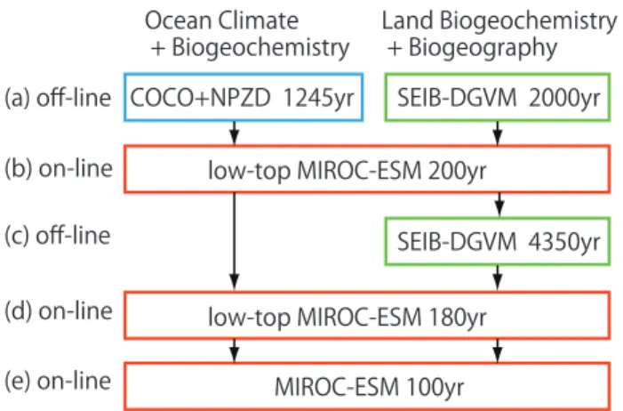
SEIB-DGVM 2000yr COCO+NPZD 1245yr
(a) off-line
Ocean Climate
+ Biogeochemistry Land Biogeochemistry + Biogeography
(b) on-line
(d) on-line
low-top MIROC-ESM 200yr
low-top MIROC-ESM 180yr
SEIB-DGVM 4350yr (c) off-line
MIROC-ESM 100yr (e) on-line
Fig. 3.Spin-up procedures of MIROC-ESM.
initial conditions, and the on-line terrestrial and ocean car-bon cycles were integrated for 200 yr (Fig. 3b). The resul-tant terrestrial carbon cycle state was again input into the off-line SEIB-DGVM, which was integrated for 4350 yr to adapt to the land-use corresponding to 1850 (Fig. 3c). Using the terrestrial carbon cycle data, the second on-line spin-up was conducted using the low-top MIROC-ESM for 180 yr (Fig. 3d), from which the final states of carbon cycle are used as the initial conditions for the final on-line spin-up of MIROC-ESM with the L80-AGCM (Fig. 3e).
In the course of the spin-up runs, we monitored representa-tive states and fluxes in the physical climate and carbon cycle components, for example, surface air temperatures, radiation fluxes at the top of atmosphere, strength of the thermohaline circulation, sea-ice extent, soil and vegetation carbon stor-age, land and ocean carbon uptakes, and so many. Each of the spin-up runs was continued until linear trends of those quantities in the last 50 yr became insignificant. After the spin-up had finished, we conducted the pre-industrial control run of MIROC-ESM for 530 yr, and the first day of the 20th year of the control run was used as the initial condition of the chemistry coupled spin-up of MIROC-ESM-CHEM, which is described in the next paragraph.
The atmospheric chemistry component (CHASER) of MIROC-ESM-CHEM was spun-up separately from the car-bon cycles because the atmospheric chemistry does not need thousands of years to reach equilibrium. Some chemical species important in the stratosphere required a few tens of years to reach equilibrium if the surface emission of source gases was substantially changed. Since we had only run the current version of CHASER under present-day condi-tions before CMIP5, we first needed to prepare appropri-ate initial conditions for 1850 utilizing the existing present-day dataset: (1) concentrations of halogen compounds such as halocarbons, inorganic chlorine and bromine were set to zero, (2) concentrations of the nitrogen family such as ni-trogen dioxide was scaled on the basis of present-day values
with reference to the surface concentration of nitrous oxide, and (3) concentration of methane and moisture were scaled with reference to the surface concentration of methane. Af-ter a spin-up of about 15 yr, the concentrations of all chem-ical compounds in the troposphere and stratosphere reached equilibrium. The chemistry spin-up run was continued for 28 yr, and the final states of the chemistry tracers were added to the initial condition of the carbon cycles described in the previous paragraph.
Finally, a fully-coupled carbon cycles-chemistry spin-up run was performed for 4 yr to derive the initial condition of the historical simulation, whose results are described in Sect. 4. This short final spin-up run was possible because: (1) the pre-industrial mean climate of MIROC-ESM that is used for the carbon cycle spin-up and of MIROC-ESM-CHEM was actually similar to each other, because ozone dis-tribution in these models is similar. (2) The present version of MIROC-ESM-CHEM does not include any direct coupling between the carbon cycles and atmospheric chemistry. The atmospheric chemistry indirectly affects ecosystems through chemistry-climate interactions. At least, we did not find any apparent changes in ecosystems before and after the chem-istry coupling.
3.2 Experimental designs
The historical simulation was performed for the period from 1850 to 2005 using a set of external forcings recommended by the CMIP5 project. Spectral changes in solar irradi-ance are considered according to Lean et al. (2005). His-torical changes in optical thickness of volcanic stratospheric aerosols are given by Sato et al. (1993) and subsequent up-dates (http://data.giss.nasa.gov/modelforce/strataer/). Unlike our previous simulations, the temporal evolution of the opti-cal thickness in latitude-altitude cross section is considered. From 1998, the optical thickness of volcanic stratospheric aerosols is exponentially reduced with one year relaxation time. In CMIP5 simulations, CHASER and SPRINTARS do not calculate stratospheric background aerosols made from carbonyl sulfide. The optical thickness of volcanic strato-spheric aerosols does include the stratostrato-spheric background aerosols, and we use it in radiation calculations and hetero-geneous chemistry calculations as the optical thickness per unit altitude can be converted into surface area density of aerosols. Atmospheric concentrations of well-mixed green-house gases are provided by Meinshausen et al. (2011). Sur-face emissions of tropospheric aerosols and ozone precursors are provided by Lamarque et al. (2010).
of four RCP socioeconomic studies (IMAGE, MINICAM, AIM, and MESSAGE) and historical data (1500–2005). The original harmonized land-use data were converted to T42 to fit the spatial resolution of this study by taking weighted means. The quality of the conversion was checked graphi-cally. Implementation of RCPs in SEIB-DGVM is described in Sect. 2.3.2.
4 Results of historical simulation
4.1 Transient variations
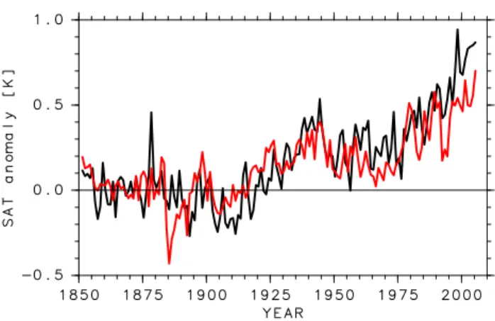
Temporal variations of global and annual mean surface air temperature (SAT) are shown in Fig. 4 for the MIROC-ESM-CHEM simulation as well as for the observations (Brohan et al., 2006). The MIROC-ESM-CHEM simulation well captures the observed multi-decadal variations throughout the whole simulation period, although the simulated SAT is about 0.2∼0.3 K cooler than observations since the Pinatubo
eruption. The simulated SAT increase in the first and the sec-ond half of the 20th century is about 0.8 and 1.0 K century−1 respectively, which is slightly less than that in the observa-tions. These global annual mean SAT trends are similar to those of our previous simulations (Nozawa et al., 2007), al-though we use different forcing datasets than previously.
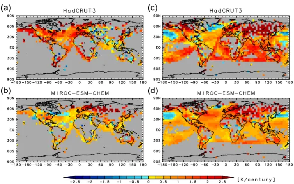
Figure 5 shows the geographical distributions of linear SAT trends for the first and second half of the 20th cen-tury. For the first half of the 20th century (Fig. 5a and b), the simulated SAT trends are about 1/2 or smaller than observa-tions over the ocean. The simulated SAT trends are positive over Eurasia despite the observed SAT trends are generally negative. For the second half of the 20th century (Fig. 5c and d), on the other hand, the overall SAT trend for the MIROC-ESM-CHEM simulation shows a realistic geograph-ical pattern, as compared to the observed one: the simulated SAT trend pattern over the northern Pacific is very similar to that in observations, although the simulated trends over the Southern Hemisphere are about 1 K century−1smaller than those in observations.
4.2 Climatology in the late 20th century
Figure 6a and b shows geographical distributions of SAT averaged for the 1961–1990 periods for the MIROC-ESM-CHEM simulation and its biases against observational dataset (Jones et al., 1999), respectively. Overall, MIROC-ESM-CHEM SAT distributions are realistic but their differ-ences from observations show systematic biases: the sim-ulated SAT is warmer in the mid and high latitudes of the Northern Hemisphere and over Antarctica. On the other hand, the simulated SAT is about 1∼2 K cooler in the tropics
and in the mid latitudes of the Southern Hemisphere. The MIROC-ESM-CHEM shows a realistic distribution of annual mean precipitation for the 1981–2000 period (Fig. 6c). However, there are some differences compared
Fig. 4.Temporal variations of global annual mean surface air tem-perature (SAT). Anomalies from the 1851–1900 mean for the ob-servations (Brohan et al., 2006; black line) and the MIROC-ESM-CHEM simulation (red line). In calculating the global annual mean SAT, modeled data are projected onto the same resolution as the observations, discarding simulated data at grid points where there was missing observational data. At each location, more than two months of data were required to calculate the seasonal mean value, and all four seasons of data were required to calculate the annual mean value.
with the GPCP observational dataset (Adler et al., 2003) (Fig. 6d): the precipitation is underestimated along the South Pacific convergence zone (SPCZ), over the eastern side of the Maritime Continent, and over Central America, whereas it is overestimated over the Maritime Continent, the north-western Indian Ocean, and the north-western side of South Amer-ica. These shortcomings are similar to those in our previous model (MIROC3.2) because these two models have almost the same atmospheric physics components.
There is significant interest in how many years the Arc-tic and AntarcArc-tic sea-ice can last in a warming globe. Sup-posing a slightly warming ocean, both the sea-ice extent and the surface albedo would decrease and more solar radiation would be absorbed by the ocean, and hence initial warming is accelerated. Therefore, Arctic and Antarctic sea-ice are very sensitive in a changing climate and can provide a good benchmark for a climate model.
Figure 7 compares the sea-ice concentration between the reanalysis (Reynolds et al., 2002) and simulation by seasons and hemispheres. MIROC-ESM-CHEM reasonably simu-lates the sea-ice seasonality in both hemispheres. The sea-ice distribution is similar between the reanalysis and simulation. During the boreal summer (JJA), the Arctic Ocean has less sea-ice and the Southern Ocean has more sea-ice compared with the other seasons, and vice versa for the boreal win-ter (DJF).
(a)
(c)
(b)
(d)
Fig. 5.Geographical distributions of linear surface air temperature trends (K century−1) in the(a, b)first and(c, d)second half of the 20th century for the(a, c)observations (Brohan et al., 2006) and(b, d)the MIROC-ESM-CHEM simulation. Trends were calculated from annual mean values only for those grid points where the annual data is available in at least 2/3 of the 50 yr and distributed in time without significant bias.
southwestern Okhotskoe Sea and northern Barrentsovo Sea also have less sea-ice during the boreal winter in the sim-ulation. Therefore, MIROC-ESM-CHEM underestimates a small amount of sea-ice over shallow oceans and such sea-ice may have disappeared by the 1990s, a bit earlier than in the observations, but the model adequately resolves most other sea-ice, which has more importance in a large-scale climate simulation.
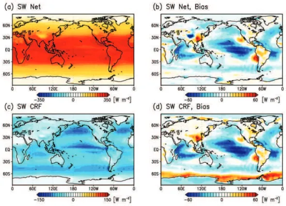
The annual mean shortwave (SW) and longwave (LW) ra-diation at the top of the atmosphere (TOA), and their cloud radiative forcing (CRF) are shown in Figs. 8 and 9. The ob-servational dataset from the Earth Radiation Budget Experi-ment (ERBE), Earth Radiant Fluxes and Albedo for Month S-9 for the period 1986 to 1990 (Barkstrom et al., 1989) is used for comparison with the model simulation. As shown in Fig. 8, negative bias in SW radiation (the model has too much reflection) and CRF can be seen in the central Pacific, western Atlantic, and Indian Ocean, and positive bias is seen in the eastern Pacific and Atlantic. These features are similar to the bias of low-level cloud albedo in Fig. 12 of Yokohata et al. (2010), and thus these biases are likely caused by the model feature of low-level cloud.
As for LW radiation, the bias is relatively small compared to that in SW radiation. A positive bias in LW radiation and LW CRF can be seen over the intertropical convergence zone (ITCZ) in the equatorial Pacific. Since this feature is similar to that of the precipitation bias shown in Fig. 6d,
this positive bias in LW radiation is likely caused by a prob-lem with the model precipitation or convection. Similarly, the negative bias in the LW radiation and LW CRF over the SPCZ may be related to the negative precipitation bias there (Fig. 6d).
The meridional cross sections of simulated zonal mean temperatures, specific humidity, and relative humidity are shown in Fig. 10, along with those biases against ERA-40 (Uppala et al., 2005). A cold bias is seen near the surface except in the Arctic. This is consistent with that in SAT (Fig. 6b). At higher altitudes, a cold bias is seen in the mid-dle troposphere between 40◦N and 50◦S, and a larger cold bias is seen in the extratropical upper troposphere and lower stratosphere.
A large negative (dry) bias is seen in the lower tropo-sphere, especially at latitudes lower than 30 degrees. Rea-sons for the dry bias in these regions are related to the cold bias near the surface (Fig. 10b) and the dry bias in the relative humidity centered around 850 hPa (Fig. 10d). In the region where the dry bias in relative humidity is maximal, the dry bias in specific humidity is also maximal. In the upper tro-posphere and lower stratosphere, a large positive (wet) bias in relative humidity is seen. This bias could cause the nega-tive temperature bias (Fig. 10b) owing to an increase in LW emission to outer space.
Fig. 6. (a)Annual mean climatology of surface air temperature (SAT) for the 1961–1990 period for the MIROC-ESM-CHEM simulations and(b)biases in the annual mean SAT climatology against the observational dataset (Jones et al., 1999).(c)Annual mean climatology of precipitation for the 1981–2000 period for the MIROC-ESM-CHEM simulations and(d)biases in the annual mean precipitation climatology against the GPCP observational dataset (Adler et al., 2003).
with those for ERA-40 (below 1 hPa) and the 1986 Com-mittee on Space Research (COSPAR) International Refer-ence Atmosphere (CIRA) data (above 1 hPa) (Fleming et al., 1990). The model qualitatively reproduces the observed meridional structure of the zonal mean winds and temper-atures in each month (January, April, July, and October). Relatively large discrepancies between the model and obser-vations are found in the winter hemisphere high latitudes. More frequent occurrence of stratospheric sudden warming than that in the observations in the 1990s results in weak winds in the northern winter upper stratosphere and meso-sphere (Fig. 11a). Less gravity wave drag owing to a lack of lateral propagation in gravity wave drag parameterizations causes strong winds in the southern winter upper stratosphere and mesosphere (Fig. 11e, see Watanabe, 2008).
Figure 12 compares time-height cross-sections for the re-analysis (ERA-40) and simulated equatorial eastward winds. They both show alternation of downward propagating east-ward and westeast-ward wind shear zones, known as the equa-torial QBO. The mean periods of the observed and sim-ulated QBO are similar to each other, i.e. approximately 28 months, while the simulated QBO behavior is somewhat
regular compared to the reanalysis. This might be due to the constant gravity wave source specified in the tropics (Sect. 2.1.1). Otherwise, it could be attributed to less vari-ability of resolved wave forcing and/or of the equatorial mean upward motions. The QBO in MIROC-ESM will be detailed in a forthcoming paper (Watanabe and Kawatani, 2011).
4.3 Aerosols
Fig. 7.Seasonal climatology of Arctic and Antarctic sea-ice concentration in the 1990s: for the boreal (JJA) and austral (DJF) summer, and the reanalysis (OISST) and simulation (MIROC-ESM-CHEM).
to rapid industrialization and deforestation. Global mean aerosol mass in the atmosphere at the end of the 20th cen-tury is about three times and twice as large as that in 1850 for BC and sulfate, respectively. Atmospheric dust slightly increased in the 20th century relative to the previous century. Anthropogenic aerosols from urban areas in the mid-latitudes of the Northern Hemisphere concentrate in the boundary layer, while biomass burning aerosols from tropical and sub-tropical regions are injected to higher altitudes due to convec-tion and fire heat (Fig. 15). Figure 16 shows the direct radia-tive forcing at the tropopause due to anthropogenic aerosols under all-sky condition, which have strong negative values over industrialized and biomass burning regions. The radia-tive forcings of the direct and indirect effects due to anthro-pogenic aerosols are−0.2 W m−2 and−0.9 W m−2 for the global mean, respectively.
4.4 Atmospheric chemistry
Figure 17 displays the temporal evolution of the global mean ozone column reproduced by our past simulation with MIROC-ESM-CHEM using the RCP dataset for CMIP5. The total ozone column rapidly decreases after 1980 in re-sponse to the increased halogen loading, exhibiting the large influence of volcanic eruptions in 1980s and 90s. The de-creasing trend of total ozone in 1980s, however, appears to
Fig. 8. Annual mean net downward(a, b)shortwave (SW) radiation at the top of the atmosphere (TOA), and(c, d)SW cloud radiative forcing (CRF) at the TOA. Results of the model simulation are shown in(a, c), and the model bias against ERBE observations (Barkstrom et al., 1989) is shown in(b, d)(see text).
experiment (Gauss et al., 2006). The spatial and seasonal dis-tributions of tropospheric ozone calculated by the model are well consistent with the GOME observations (Fig. 18). Both the model and observation show large ozone increases in the northern mid-latitudes in spring (MAM) due to enhanced chemical production of ozone and downward transport of stratospheric ozone. In summer in the Northern Hemisphere, the model well captures the ozone enhancements over the continental regions of Eurasia and North America. In spring time for the Southern Hemisphere (SON), outflow of high ozone in the mid-latitudes from biomass burning in South America and Africa is also well reproduced by the model. On the other hand, the model appears to underestimate ozone abundances in the northern high latitudes, including the Arc-tic for spring and summer. We found that this underestima-tion of tropospheric ozone partly compensates for the gen-eral overestimation of the column ozone amount in the north-ern high latitudes as described above. These features of our model simulation suggest that further improvement and vali-dation of chemical processes are still required for the model-ing framework of MIROC-ESM-CHEM.
4.5 Land surface and terrestrial ecosystems
Fig. 9.Annual mean net downward(a, b)longwave (LW) radiation at the top of the atmosphere (TOA), and(c, d)SW cloud radiative forcing (CRF) at the TOA. Results of the model simulation are shown in(a, c), and the model bias against ERBE observations (Barkstrom et al., 1989) is shown in(b, d)(see text).
nomadic livestock as well as the pasture that is enclosed. Total vegetation biomass consisting of leaf, stem, and root was 353 Pg C for the 2000–2005 average, which is at the lower end of previous reports: 560 Pg C in Ajtay et al. (1979), 359 Pg C in Dixon et al. (1994), and 466–654 Pg C in Pren-tice et al. (2001). This is because artificial disturbances to vegetation carbon through land use change, forest cutting, gradual forest recovery from abandoned agricultural area, an-nual harvesting of crops, continuous livestock grazing in pas-ture and its recovery, are incorporated in the present model, while previous models deal with the potential vegetation only in the absence of artificial disturbance (Friedlingstein et al., 2006; Sitch et al., 2008) or only consider the natural vegeta-tion and croplands (Kato et al., 2009; Matthews et al., 2005; Meissner et al., 2003). As a result, the predicted value of veg-etation carbon tends to be lower than that of previous appli-cations of terrestrial ecosystem models. Recent aggregated results of forest statics considering human impacts revealed that the forest carbon stock is less than 300 Pg C (Kinder-mann et al., 2008), which is even lower than the 338 Pg C estimated from our model.
The distribution pattern of forest biomass based on obser-vations and reproduced by MIROC-ESM-CHEM are shown in (Fig. 19b and c). Forest carbon in the tropical regions such as South America and Africa carbon was generally
underpredicted, while the South and Southeast Asia were overestimated. The extent of forests and moderate accumu-lations of carbon in temperate and boreal regions were well reproduced. Regions with low forest biomass are located in deserts, semi-arid regions, and agricultural areas of Europe, Asia, and North America. Although the model can correctly predict the location of deserts in the Northern Hemisphere, it failed to capture the semi-arid or desert areas in Australia and steppe and savanna in southern Africa. This failure is due to the high sensitivity of plants to soil moisture in the terrestrial ecosystem model and a positive precipitation bias in these areas.
Fig. 10.Zonal mean of annual averaged model climatology (1980–1999) for(a)atmospheric temperature,(c)specific humidity, and(e) rel-ative humidity. Differences between the model climatology and ERA-40 data are displayed in(b),(d), and(f), respectively.
2009) and the amounts of soil organic carbon estimated by the model is strongly affected by it’s settings (e.g. the num-ber of soil pool, turnover rate in decomposition, and effects from soil water and temperature). In addition, as the mech-anisms for the high accumulation of soil carbon like frozen carbon or peat in the north circumpolar regions are not well known, global terrestrial ecosystem models represent these processes implicitly with the lack of precise mechanism of the interaction between physical environment and soil car-bon dynamics.
The model was able to capture the global trend of large accumulations of soil organic carbon in boreal and tundra regions in Eurasia and North America, and small accumula-tions in tropical and extra-tropical regions (Fig. 19e). Com-pared with the observation (IGBP-DIS, 2000; Fig. 19d), the model overestimated the soil carbon in mountainous or plateau areas such as the Rocky Mountain, Tibetan plateau, and a chain of mountains in east Siberia, likely due to the overestimation of vegetation biomass. The reason for these overestimate in vegetation carbon is that the growth
160 180 200 220 240 260 280 300 Temperature [K]
(a) (b)
(c) (d)
(e) (f)
(g) (h)
MIROC-ESM-CHEM
(a)
(b)
-60 -50 -40 -30 -20 -10 0 10 20 30 40 50 60 Eastward wind [ms-1]
Fig. 12.Zonal-mean zonal winds over the equator for(a)ERA-40 and(b)the model result.
Fig. 13. Anomaly of the aerosol optical thickness averaged for the period 1991–2000 relative to the period 1851-1860.
respiration and gross land use emissions) was 62.8 Pg C yr−1. The resultant net carbon fluxes from the atmosphere to land (net biome production) in the 1990s and 2000–2005 were 1.34 and 1.50 Pg C yr−1, respectively, which are within the range reported by Denman et al. (2007).
Fig. 15.Anomaly of the zonal-mean aerosol extinction coefficient averaged for the period 1991–2000 relative to the period 1851– 1860.
Fig. 16.Annual mean radiative forcing of the aerosol direct effect under all-sky conditions in the year 2000 relative to 1850.
In MIROC-ESM-CHEM, the distribution and communi-ties of vegetation, biomass, and the leaf amount are dynam-ically determined by SEIB-DGVM. It is therefore impor-tant to reproduce the relation between climate and terrestrial ecosystems properly in evaluating the climate sensitivity in-cluding those feedback processes. Suzuki et al. (2006) ex-amined the relation between climate zones and vegetation distribution using the global observation datasets. The cli-matological condition for vegetation growth was evaluated by the warmth index (WAI) and the wetness index (WEI), and they were compared with the normalized difference veg-etation index (NDVI), which represents the greenness of land ecosystems. Figure 20a is a scatter plot of the WEI and the WAI with the color tones according to the NDVI, after Fig. 2
Fig. 17. Time series of global mean total and tropospheric ozone column abundance in Dobson Units simulated by the MIROC-ESM-CHEM (blue and red lines, respectively). Triangles represent tropospheric column ozone derived from satellite measurements (GOME) for around 2000.
of Suzuki et al. (2006). The NDVI was large where both WEI and WAI were high, while the NDVI was small where either the WEI or the WAI were low.
Figure 20b shows a scatter plot of WEI and WAI with color tones according to the LAI calculated by MIROC-ESM-CHEM. The colors for the logarithmic LAI are adapted to follow the colors for the NDVI in Fig. 20a, since the in-creasing rate of NDVI is generally lower for larger LAI. (My-neni et al., 2002). The general shape of the scatter plot for WEI and WAI is similar to that in Fig. 20a. MIROC-ESM-CHEM also reproduces the features of large LAI in regions where WEI and WAI are high, and small LAI where WEI or WAI is low. However, points with a small WAI and a large WEI were fewer than observation. That is probably due to the overestimation of surface air temperature in the warm season over the continents in MIROC-ESM-CHEM.
4.6 Ocean and marine ecosystems
Fig. 18. Tropospheric column ozone distributions(a)observed by GOME for 2000 and(b)calculated by the model for distinct seasons. The modeled ozone is shown as an average of simulations for 2000–2003 (using the averaging kernel for GOME 2000).
describes a W-shape for a few hundred meters depth from the surface.
The next layer of subsurface water is called Antarctic In-termediate Water (AAIW), which slides down from the sur-face in the Southern Ocean to 1 km depth in the tropics. The AAIW is relatively fresh (low salinity), rich in nutrients, and the lowest in temperature at around 100–200 m depth.
Below the AAIW, at a depth of 1000–4000 m, the North Atlantic Deep Water (NADW) fills most of the Atlantic basin with more saline and low nutrient water which originates from the high northern latitudes, but reaches as far south as 40◦S and beyond.
At the bottom of the Atlantic Ocean, the Antarctic Bottom Water (AABW) consists of the coldest and nutrient rich but less saline water.
Compared to the observations (Conkright et al., 2002), the AAIW and AABW are reasonably well simulated by the model, while the NADW looks to be weakly formed, prob-ably due to stable stratification near the surface. The At-lantic meridional overturning cell is also somewhat weakly resolved, as the maximum stream function across 30◦N is around 15±1 Sv, but is still in a valid range.
Phytoplankton are the microscopic organisms respon-sible for ocean primary production, and play an impor-tant role in controlling the ocean-atmosphere CO2 flux, and hence the global carbon cycle. In order to validate the biogeochemistry-capable general circulation model, the spatio-temporal variability of phytoplankton is analyzed.
Figure 22 illustrates the seasonal variation of sea surface chlorophyll in the central Pacific, around the international dateline. Both the satellite observation and model simulation show the sinusoidal curves of meridional migration with time because the solar insolation is a factor for the chlorophyll
growth. Another chlorophyll growth factor is the nutrient supply. The phytoplankton spring bloom initiates around March (October) in the North (South) subpolar Pacific, as so-lar insolation and the nutrient supply increases and the verti-cal mixing activates. The North (South) Pacific spring bloom is underestimated (overestimated) in the simulation mainly due to the underestimated (overestimated) nutrient distribu-tions beneath.
Other biases are visible at the equator and around 15◦N.
These biases are caused by unrealistic strong trade winds in the central to western Pacific which often appear in atmosphere-ocean coupled general circulation models. The anomalous strong easterly winds further enhance the equato-rial upwelling and the development of a cold tongue in the boreal summer, and also enhance upwelling where the east-erly wind velocity is at a maximum, by enhancing the north-ward (southnorth-ward) transport to the north (south).
In summary, some biases are found in the ocean circulation model simulation results but these arise from errors in inputs from other components of the model, and all are reasonable. The seasonality in ocean processes is fairly well simulated.
5 Concluding remarks
Fig. 20. (a)Observation-based relation of WEI (wetness index), WAI (warmth index), and NDVI (normalized differential vegetation index) over the global continents at 1 degree resolution. The NDVI value is shown by color at the intersection of WEI and WAI.(b)As in(a), but for the model result. The colors are for the logarithmic LAI, and at the model resolution (T42).
Fig. 21. Annual mean climatology of the Atlantic latitude-depth sector at 25◦W: sea water potential temperature (T, degC), salin-ity (S, PSU), and nutrients (N, mmol N m−3), for the observations (WOA01) (left column) and simulation (MIROC-ESM-CHEM) (right column).
Fig. 22. Time-latitude Hovmoeller diagram of the sea surface chlorophyll density (mg Chl m−3) around the international date-line (zonally averaged for 170◦E–170◦W) for(a)satellite obser-vation (SeaWiFS) and(b)the simulation (MIROC-ESM-CHEM). Note that the satellite observation is missing data in the polar night or under sea-ice because the SeaWiFS measures the chlorophyll re-motely by the ocean surface color.
climatology of the zonal-mean zonal winds and temperatures in the stratosphere and mesosphere generally agree with the observations, and the model self-consistently generates the equatorial QBO in the lower stratosphere. The aerosol mod-ule simulates the historical evolution of aerosols in terms of changes in the optical thickness, column mass loading, ex-tinction coefficient, and direct effect, based on the RCP his-torical emissions. The simulated present-day tropospheric column ozone distribution shows reasonable agreement with satellite observations, although several systematic errors are pointed out. The terrestrial carbon cycle component simu-lates realistic geographical distributions of LAI, GPP, veg-etation biomass, and soil organic carbon. The ocean GCM and marine biogeochemistry component generally simulates the observed latitude-depth distributions of potential temper-atures, salinity, and nutrients in the Atlantic sector, as well as seasonal variations in chlorophyll over the Pacific sector.
Overall, MIROC-ESM-CHEM generally shows good per-formance in the reproduction of the earth system in the his-torical period. The model has also been used for several mandatory simulations of CMIP5, while the atmospheric chemistry uncoupled version (MIROC-ESM) has been used to conduct a wider variety of simulations. Although the general results of MIROC-ESM and MIROC-ESM-CHEM agree with each other in terms of historical evolution of SAT, aerosols, sea-ice, land surface, and the terrestrial and ma-rine biogeochemistry, there are several fundamental differ-ences between the two versions. For instance, ozone con-centration is predicted in MIROC-ESM-CHEM, while pre-scribed in MIROC-ESM. The prepre-scribed ozone includes ef-fects of historical evolution of tropospheric ozone precursors and halogen species destroying the stratospheric ozone, but effects of the solar cycle and QBO on the ozone concentra-tion are neglected in the current setup (Kawase et al., 2011). In this context, MIROC-ESM-CHEM seems to have a higher potential to realistically reproduce climate variability in the stratosphere. Further evaluations of the simulated climate fields are required for both versions, along with the simu-lated biogeochemistry parameters.
Several papers on the analyses of our CMIP5 simulations have already been published in peer-reviewed journals. For example, Watanabe et al. (2011) and Watanabe and Yoko-hata (2011) demonstrate the projected future evolution of the surface ultraviolet radiation and attribute its potential changes to future changes in column ozone, aerosols, clouds, and surface albedo. Watanabe and Kawatani (2011) focus on the future evolution of the equatorial QBO associated with climate change.
Acknowledgements. The authors would like to thank two referees
for their constructive comments on the original manuscript. They also thank Team-MIROC for their support and encouragement throughout the project. Discussions with Hideharu Akiyoshi were helpful to improve the atmospheric chemistry component. We thank Rikie Suzuki for providing the global datasets of observation-based climatology and vegetation indices. This study
was supported by the Innovative Program of Climate Change Projection for the 21st century, MEXT, Japan. The numerical simulations in this study were performed using the Earth Simulator, and figures were drawn using GTOOL and the GFD-DENNOU Library. This study is supported in part by the Funding Program for Next Generation World-Leading Researchers by the Cabinet Office, Government of Japan (GR079).
Edited by: O. Boucher
References
Adler, R. F., Huffman, G. J., Chang, A., Ferraro, R., Xie, P., Janowiak, J., Rudolf, B., Schneider, U., Curtis, S., Bolvin, D., Gruber, A., Susskind, J., and Arkin, P.: The Version 2 Global Precipitation Climatology Project (GPCP) Monthly Precipitation Analysis (1979–Present), J. Hydrometeor., 4, 1147–1167, 2003. Ajtay, G. L., Kenter, P., and Duvigneaud, P.: Terrestrial primary
production and phytomass, in: The Global Carbon Cycle, edited by: Bolin, B., Degens, E. T., Kempe, S., and Ketner, P., New York, USA, John Wiley & Sons, 129–181, 1979.
Akiyoshi, H., Sugita, T., Kanzawa, H., and Kawamoto, N.: Ozone perturbations in the Arctic summer lower stratosphere as a re-flectio in of NOx chemistry and wave activity, J. Geopys. Res., 109(D03), D03304, doi:10.1029/2003JD003632, 2004. Aoki, T., Motoyoshi, H., Kodama, Y., Yasunari, T. J., Sugiura, K.,
and Kobayashi, H.: Atmospheric Aerosol Deposition on Snow Surfaces and Its Effect on Albedo, Sci. Online Lett. Atmos., 2, 13–16. doi:10.2151/sola.2006-004, 2006.
Arakawa, A. and Schubert, W. H.: Interactions of cu-mulus cloud ensemble with the large-scale environment, Part I, J. Atmos. Sci., 31, 674–701, doi:10.1175/1520-0469(1974)031<0674:IOACCE>2.0.CO;2, 1974.
Barkstrom, B. R., Harrison, E. F., Smith, G., Green, R., Kibler, J., Cess, R., and ERBE Science Team: Earth Radiation Budget Experiment (ERBE) archival and results, B. Am. Meteorol. Soc., 70, 1254–1262, April 1985, 1989.
Batjes, N. H.: Total carbon and nitrogen in the soils of the world, Euro. J. Soil Sci., 47, 151–163, 1996.
Bonan, G. B.: Forests and climate change: Forcings, feedbacks, and the climate benefits of forests, Science, 320, 1444-1449, doi:10.1126/science.1155121, 2008.
Bougamont, M., Bamber, J. L., and Greuell, W.: A surface mass balance model for the Greenland Ice Sheet, J. Geophys. Res., 110, F04018, doi:10.1029/2005JF000348, 2005.
Brasseur, G. P., Hauglustaine, D. A., Walters, S., and Rasch, P. J.: MOZART, a global chemical transport model for ozone and re-lated chemical tracers, 1. Model description, J. Geophys. Res., 103, 28265–28289, 1998.
Brohan, P., Kennedy, J. J., Harris, I., Tett, S. F. B., and Jones, P. D.: Uncertainty estimates in regional and global observed tempera-ture changes: A new data set from 1850, J. Geophys. Res., 111, D12106, doi:10.1029/2005JD006548, 2006.
Coleman, K. and Jenkinson, D. S.: ROTHC-26.3, A model for the turnover of carbon in soils, available at: http://www. rothamsted.bbsrc.ac.uk/Research/Centres/home.php, last access: 2010, 1999.
At-las 2001: Objective Analyses, Data Statistics, and Figures, CD-ROM Documentation, National Oceanographic Data Center, Sil-ver Spring, MD, 17 pp., 2002.
Cox, P., Betts, R., Jones, C., Spall, S., and Totterdell, I.: Accel-eration of global warming due to carbon-cycle feed-backs in a coupled climate model, Nature, 408, 184–187, 2000.
Cramer, W., Kicklighter, D. W., Bondeau, A., Moore III, B., Churk-ina, G., Nemry B., Ruimy, A., Schloss, A. L., and the participants of the Potsdam NPP model intercomparison: Comparing global models of terrestrial net primary productivity (NPP): overview and key results, Glob. Change Biol., 5, 1–15, 1999.
Denman, K. L., Brasseur, G., Chidthaisong, A., Ciais, P., Cox, P. M., Dickinson, R. E., Hauglustaine, D., Heinze, C., Holland, E., Jacob, D., Lohmann, U., Ramachandran, S., da Silva Dias, P. L., Wofsy, S. C., and Zhang, X.: Couplings Between Changes in the Climate System and Biogeochemistry, in: Climate Change 2007: The Physical Science Basis. Contribution of Working Group I to the Fourth Assessment Report of the Intergovernmental Panel on Climate Chnage, edited by: Solomon, S., Qin, D., Manning, M., Chen, Z., Marquis, M., Averyt, K. B., Tignor, M., and Miller, H. L., Cambridge University Press, Cambridge, United Kingdom and New York, NY, USA, 499–588, 2007.
Dixon, R. K., Brown, S., Houghton, R. A., Solomon, A. M., Trexler, M. C., and Wisniewski, J.: Carbon Pools and Flux of Global Forest Ecosystems, Science, 263, 185–190, 1994.
Emori, S., Nozawa, T., Numaguchi, A., and Uno I., Impor-tance of cumulus parameterization for precipitation simulation over east Asia in June, J. Meteorol. Soc. Jpn., 79, 939–947, doi:10.2151/jmsj.79.939, 2001.
Fleming, E. L., Chandra, S., Barnett, J. J., and Corney, M.: Zonal mean temperature, pressure, zonal wind, and geopotential height as functions of latitude, COSPAR International Reference Atmo-sphere: 1986, part II: Middle atmosphere Models, Adv. Space Res., 10, 11–59, doi:10.1016/0273-1177(90)90386-E, 1990. Fountoukis, C. and Nenes, A.: ISORROPIA II: a
com-putationally efficient thermodynamic equilibrium model for K+Ca+2Mg+2NH+4Na+SO24−NO−3Cl−H2O aerosols, Atmos. Chem. Phys., 7, 4639–4659, doi:10.5194/acp-7-4639-2007, 2007.
Friedlingstein, P., Cox, P., Betts, R., Bopp, L., von Bloh, W., Brovkin, V., Cadule, P., Doney, S., Eby, M., Fung, I., Bala, G., John, J., Jones, C., Joos, F., Kato, T., Kawamiya, M., Knorr, W., Lindsay, K., Matthews, H. D., Raddatz, T., Rayner, P., Reick, C., Roeckner, E., Schnitzler, K.-G., Schnur, R., Strassmann, K., Weaver, A. J., Yoshikawa, C., and Zeng, N.: Climate-carbon cy-cle feedback analysis: Results from the C4MIP model intercom-parison, J. Clim., 19(14), 3337–3353, doi:10.1175/JCLI3800.1, 2006.
Gauss, M., Myhre, G., Isaksen, I. S. A., Grewe, V., Pitari, G., Wild, O., Collins, W. J., Dentener, F. J., Ellingsen, K., Gohar, L. K., Hauglustaine, D. A., Iachetti, D., Lamarque, F., Mancini, E., Mickley, L. J., Prather, M. J., Pyle, J. A., Sanderson, M. G., Shine, K. P., Stevenson, D. S., Sudo, K., Szopa, S., and Zeng, G.: Radiative forcing since preindustrial times due to ozone change in the troposphere and the lower stratosphere, Atmos. Chem. Phys., 6, 575–599, doi:10.5194/acp-6-575-2006, 2006.
Hunke, E. and Dukowicz, J. K.: An elastic-viscous-plastic model for sea ice dynamics, J. Phys. Oceanogr., 27, 1849–1867, 1997. Hibbard, K. A., Meehl, G. A., Cox, P., and Friedlingstein, P.:
A strategy for climate change stabilization experiments, EOS, T. Ame. Geophys. Union, 88(20), doi:10.1029/2007EO200002, 2007.
Hill, C., DeLuca, C., Balaji, V., Suarez, M., and Da Silva, A.: The architechture of the earth system modeling framework, Comput. Sci. Eng., 6, 18-28, 2004.
Hines, C. O.: Doppler-spread parameterization of gravity wave mo-mentum deposition in the middle atmosphere, Part 2: Broad and quasi monochromatic spectra, and implementation, J. Atmos. So-lar Terr. Phys., 59, 387–400, 1997.
Houghton, R. A., Hobbie, J. E., Melillo, J. M., Moore, B., Peter-son, B. J., Shaver, G. R., and Woodwell, G. M.: Changes in the Carbon Content of Terrestrial Biota and Soils between 1860 and 1980 – a Net Release of CO2to the Atmosphere, Ecol. Monogr., 53, 235–262, 1983.
Hurtt, G. C., Chini, L. P., Frolking, S., Betts, R., Feddema, J., Fischer, G., Goldewijk, K. K., Hibbard, K., Janetos, A., Jones, C., Kindermann, G., Kinoshita, T., Riahi, K., Shevliakova, E., Smith, S., Stehfest, E., Thomson, A., Thornton, P., van Vuuren, D., and Wang, Y. P.: Harmonisation of global land-use scenarios for the period 1500–2100 for IPCC-AR5, iLEAPS Newsletter, 6–8, 2009.
IGBP-DIS (International Geosphere-Biosphere Program, Data and Information Services): Global Soil Data Products, available at: http://daac.ornl.gov/SOILS/guides/igbp-surfaces.html, last access: 2010, 2000.
IPCC: in Climate Change 2007: The Physical Science Basis, Con-tribution of Working Group I to the Fourth Assessment Report of the Intergovernmental Panel on Climate Change, edited by: Solomon, S., Qin, D., Manning, M., Chen, Z., Marquis, M., Av-eryt, K. B., Tignor, M., and Miller, H. L., Cambridge University Press, Cambridge and New York, 2007.
Ise, T. and Sato, H.: Representing subgrid-scale edaphic hetero-geneity in a large-scale ecosystem model: A case study in the circumpolar boreal regions, Geophys. Res. Lett., 35, L20407, doi:10.1029/2008gl035701, 2008.
Ise, T., Hajima, T., Sato, H., and Kato, T.: Simulating the two-way feedback between terrestrial ecosystems and climate: Im-portance of forest ecological processes on global change, in: For-est Canopies: ForFor-est Production, Ecosystem Health, and Climate Conditions, edited by: Creighton, J. D. and Roney, P. J., NOVA, New York, 111–126, 2009.
Ito, A.: Climate-related uncertainties in projections of the twenty-first century terrestrial carbon budget: off-line model experiments using IPCC greenhouse-gas scenarios and AOGCM climate projections, Clim. Dynam., 24, 435–448, doi:10.1007/s00382-004-0489-7, 2005.
Jenkin, M. E., Saunders, S. M., and Pilling, M. J.: The tropospheric degradation of volatile organic compounds: A protocol for mech-anism development, Atmos. Environ., 31, 81–104, 1997. Jobbagy, E. G. and Jackson, R. B.: The vertical distribution of soil
organic carbon and its relation to climate and vegetation, Ecol. Appl., 10, 423–436, 2000.
Jones, P. D., New, M., Parker, D. E., Martin, S., and Rigor, I. G.: Surface air temperature and its changes over the past 150 years, Rev. Geophys., 37, 173–199, 1999.