Climate change and sectors of the surface water cycle in CMIP5 projections

(1)

HESSD

11, 8537–8569, 2014

Surface water cycle in CMIP5 projections

P. A. Dirmeyer et al.

Title Page

Abstract Introduction

Conclusions References

Tables Figures

◭ ◮

Back Close

Full Screen / Esc

Printer-friendly Version Interactive Discussion

Discussion

P

a

per

|

Discus

sion

P

a

per

|

Discussion

P

a

per

|

Discussion

P

a

per

|

Hydrol. Earth Syst. Sci. Discuss., 11, 8537–8569, 2014 www.hydrol-earth-syst-sci-discuss.net/11/8537/2014/ doi:10.5194/hessd-11-8537-2014

This discussion paper is/has been under review for the journal Hydrology and Earth System Sciences (HESS). Please refer to the corresponding final paper in HESS if available.

Climate change and sectors of the

surface water cycle in CMIP5 projections

P. A. Dirmeyer, G. Fang, Z. Wang, P. Yadav, and A. D. Milton

George Mason University, 4400 University Drive, MS 6C5, Fairfax VA 22030, USA

Received: 27 June 2014 – Accepted: 1 July 2014 – Published: 25 July 2014

Correspondence to: P. A. Dirmeyer ([email protected])

(2)

HESSD

11, 8537–8569, 2014

Title Page

Tables Figures

◭ ◮

Back Close

Full Screen / Esc

Discussion

P

a

per

|

Discus

sion

P

a

per

|

Discussion

P

a

per

|

Discussion

P

a

per

|

Abstract

Results from ten global climate change models are synthesized to investigate changes in extremes, defined as wettest and driest deciles in precipitation, soil moisture and runo_ffbased on each model’s historical twentieth century simulated climatology. Un-der a moUn-derate warming scenario, regional increases in drought frequency are found

5

with little increase in floods. For more severe warming, both drought and flood become much more prevalent, with nearly the entire globe significantly affected. Soil moisture changes tend toward drying while runoff trends toward flood. To determine how dif-ferent sectors of society dependent the on various components of the surface water cycle may be affected, changes in monthly means and interannual variability are

com-10

pared to data sets of crop distribution and river basin boundaries. For precipitation, changes in interannual variability can be important even when there is little change in the long-term mean. Over 20 % of the globe is projected to experience a combination of reduced precipitation and increased variability under severe warming. There are large differences in the vulnerability of different types of crops, depending on their spatial

15

distributions. Increases in soil moisture variability are again found to be a threat even where soil moisture is not projected to decrease. The combination of increased vari-ability and greater annual discharge over many basins portends increased risk of river flooding, although a number of basins are projected to suffer surface water shortages.

1 Introduction 20

The suite of climate model simulations from the Coupled Model Intercomparison Project Phase 5 (CMIP5) offers a wealth of information about the potential for future climate change across a range of emission/mitigation scenarios. The CMIP5 simula-tions have suggested that hydrologic feedbacks of the land surface to the atmosphere are likely to intensify and the spatial and temporal extent of the regions of strong

feed-25

(3)

HESSD

11, 8537–8569, 2014

Title Page

Tables Figures

◭ ◮

Back Close

Full Screen / Esc

Discussion

P

a

per

|

Discus

sion

P

a

per

|

Discussion

P

a

per

|

Discussion

P

a

per

|

interactions are studied because of their potential implications for climate predictability and their role in hydrologic extremes. These previous results motivate us to examine how extremes in the surface water cycle are projected to change in the next century, and how they may affect specific sectors of society.

Recent studies have used the output of a small number of CMIP5 models to drive an

5

additional suite of sector models to assess changes in the likelihood of flood (Dankers et al., 2014), drought (Prudhomme et al., 2014), significant water resource impacts (Schewe et al., 2014) and agriculture (Rosenzweig et al., 2014). In such a two-step modeling approach, versions of the same land surface model are sometimes employed twice (once in the CMIP5 climate model and again as a sector model) or different

10

land surface models are convolved where inconsistencies can amplify errors (cf. Koster et al., 2009).

It is arguably a cleaner comparison to examine the CMIP5 output directly, even if sector behaviors are poorly represented or absent in the models themselves. By com-paring relevant climate outputs superposed on secondary sector datasets such as crop

15

distributions and hydrologic catchments, key drivers may be assessed in an alternative way. In this study, we examine projected changes in the extremes within aspects of the surface water cycle and their potential impacts as directly represented by the CMIP5 models. We have characterized three sectors of water cycle extremes for this study: meteorological (precipitation), hydrological (runo_ff) and agricultural (soil moisture).

20

Section 2 describes the data sets used and the specific analyses applied to those data in this study. Changes in the occurrence rates of extremes are presented in Sect. 3. Section 4 categorizes projected hydrologic changes in terms of the sectors defined above. Rainfall changes are assessed based on the spectrum of various cli-mate indices. Soil moisture changes are composited against the global coverage of

25

(4)

HESSD

11, 8537–8569, 2014

Title Page

Tables Figures

◭ ◮

Back Close

Full Screen / Esc

Discussion

P

a

per

|

Discus

sion

P

a

per

|

Discussion

P

a

per

|

Discussion

P

a

per

|

2 Data and analyses

Monthly mean fields of precipitation, total runoff, and moisture in the uppermost 10 cm of the soil from CMIP5 simulations (Taylor et al., 2012) are examined, along with av-erages of inter-annual standard deviation (IASD) based on monthly means. Data are taken from single simulations of ten different climate models, the first ensemble

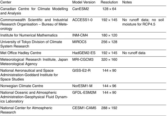
mem-5

ber in each case (r1i1p1). The ten models are listed in Table 1. Three different climate cases are considered: the transient 20th century (historical) case as well as two of the future climate scenarios; net radiative forcing scenarios of 4.5 W m−2(RCP45) and 8.5 W m−2(RCP85) (van Vuuren et al., 2011). Output from the last 90 simulated years of the three different climate cases of each model are detrended before interannual

10

variances are calculated, as described in Dirmeyer et al. (2014). All analyses are per-formed on each model’s native grid on a month-by-month basis, and then aggregated to standard three-month seasons by averaging the results across the three months, or aggregated across growing seasons for the crop-based analysis as explained below. Only multi-model statistics are shown – all multi-model means are a simple average of

15

the indicated statistic across the 10 models.

Historical thresholds for extremes are defined for each model and month at each land surface grid box. Specifically, the extreme deciles are calculated from 90 years of un-detrended data from the historical case; the thresholds would be the values for the 9th driest and 9th wettest value for each month at each point. This defines for this study

20

the contemporary 20th century definitions of “drought” and “flood” as represented by each model for each month of the year. These thresholds are then compared to the distributions derived from the RCP4.5 and RCP8.5 cases. Namely, we determine how many years out of 90 exceed the historical thresholds. Large changes indicate areas where adaptation will be critical for future water resources. Calculations are performed

25

for each month and then averaged to derive estimates for 3 month seasons.

(5)

HESSD

11, 8537–8569, 2014

Title Page

Tables Figures

◭ ◮

Back Close

Full Screen / Esc

Discussion

P

a

per

|

Discus

sion

P

a

per

|

Discussion

P

a

per

|

Discussion

P

a

per

|

hydrologic sector analysis, the CMIP5 data are interpolated onto the 1/2◦ grid of the Total RunoffIntegrated Pathways (TRIP) river routing data set of Oki et al. (1999). TRIP is also used to define the 100 largest named river basins for basin-scale assessments. For the agricultural sector analysis, the high-resolution grid matches the 1/12◦gridded crop information of Sacks et al. (2010). This is also the data set used for the global

dis-5

tribution of 19 major types of crops, as well as the mean planting and harvest dates. As explained in the documentation for that data set, crop calendar data was not available for all locations where each crop is grown. Extrapolated planting and harvest dates are provided that fill out the global grid. This information is used to define the growing sea-son at each location so that totals, averages and IASD of the multi-model water cycle

10

variables can be calculated for the growing season. Fields for extremes in the meteo-rological sector (precipitation) are also analyzed on the grid of Sacks et al. (2010).

3 Changes in extremes

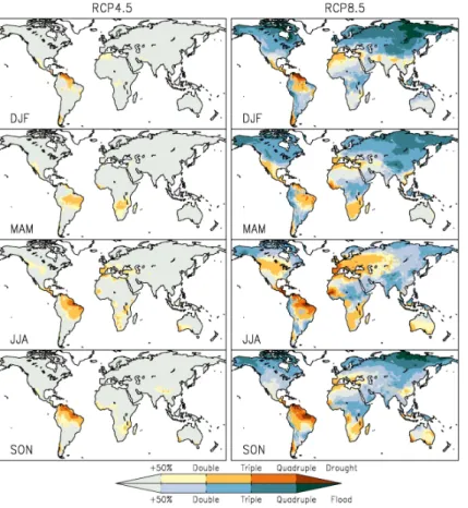
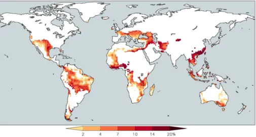
Figure 1 shows the multi-model estimates for the changes in occurrence of droughts and floods in precipitation. Shading indicates where the 20th century thresholds are

15

exceeded in at least 50, 100 (double), 200 (triple) and 300 % (quadruple) of the years (effectively 13.5, 18, 27 and 36 out of 90 years). Bootstrap tests of sampling with re-placement over 104time series simulations suggest the likelihood of falsely exceeding 50, 100 and 200 % increases in frequency of a 10 % tail with a sample size of 90 are 7.6, 0.7 and less than 0.01 % respectively. There are some locations where both

ex-20

tremes become notably more frequent; the color scales overlap in those locations. Noteworthy projected changes in the RCP4.5 case are almost all toward increased frequency of drought. There are only a few points at high northern latitudes during win-ter where the multi-model average suggests an increase in precipitation by more than 50 %. Rather, there is a stark increase in drought likelihood over much of tropical South

25

(6)

HESSD

11, 8537–8569, 2014

Title Page

Tables Figures

◭ ◮

Back Close

Full Screen / Esc

Discussion

P

a

per

|

Discus

sion

P

a

per

|

Discussion

P

a

per

|

Discussion

P

a

per

|

In the RCP8.5 case, there is hardly a region or season that is not projected to ex-perience a marked change in precipitation extremes. There are widespread increases in flood frequency at higher latitudes of the Northern Hemisphere, peaking in area and severity during DJF. Increases are also projected throughout most or all of the year over much of tropical Africa and extratropical South America, the Pacific coasts of Colombia,

5

Ecuador and Peru, Indonesia, South Asia and Tibet. Otherwise, the regions of more pervasive drought in RCP4.5 intensify and expand.

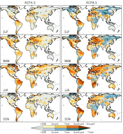
These changes are largely reflected in soil moisture as well (Fig. 2), with a shift in the zero line relative to the precipitation changes toward more drought area, reflecting the increase in evaporation that accompanies warmer temperatures. A number of

agri-10

culturally important locations are seen to su_ffer a doubling or tripling of drought in the RCP4.5 case, and even a quadrupling or more in the RCP8.5 case. Such areas include much of Eastern Europe in spring, the Great Plains of North America in summer, and the Mediterranean region year-round. Most agricultural areas of South and East Asia appear to escape escalation in drought in the RCP4.5 case, but China and Southeast

15

Asia begin to succumb in RCP8.5. Tropical South America and southern Africa appear to be hard hit in both scenarios. Wet extremes in soil moisture become much more frequent across India and surrounding nations during and after the monsoon. It is not immediately clear if this would be helpful or disruptive for agriculture – consequences would likely depend on the location and crops grown.

20

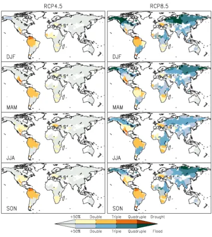
Figure 3 shows the basin-average changes in the frequency of drought and flood for the 100 largest named river basins in the TRIP data set. In RCP4.5 there is only one instance of a basin having at least a 50 % increase in flood situations – the Yukon in DJF. Otherwise, the drought regions evident in precipitation are reflected here, partic-ularly over northern South America, southern North America, Southern Europe, and

25

(7)

HESSD

11, 8537–8569, 2014

Title Page

Tables Figures

◭ ◮

Back Close

Full Screen / Esc

Discussion

P

a

per

|

Discus

sion

P

a

per

|

Discussion

P

a

per

|

Discussion

P

a

per

|

frequency distribution of precipitation favors runoff increases and reduces infiltration. Combined with greater evaporative stresses, soil moisture easily becomes depleted.

We also examined whether there were situations where drought or flood extremes moderated from RCP4.5 to RCP8.5. There are some locations and seasons for each variable where the number of years out of 90 with drought drops by 50 % or more

5

in RCP8.5 relative to RCP4.5 (expected by random chance in about 1.8 % of cases according to bootstrap simulations). These instances are mainly confined to the tropics and subtropics, and are much smaller than the area where drought years increase by 50 % or more. The area where flood extremes increase by 5 or more years from RCP4.5 to RCP8.5 covers nearly the entire globe for each season and variable, even

10

soil moisture (not shown). There are no locations where the multi-model estimates for flood extremes dropped by more than 4 cases per 90 years for any of the variables examined.

4 Sector impacts

Here we present tailored examinations of the meteorological (precipitation), agricultural

15

(soil moisture) and hydrological (runoff) sectors.

4.1 The meteorological sector

Meteorological extremes are among the simplest to quantify, as they can be based on easily measureable quantities such as temperature or precipitation. However, they are somewhat removed from the tangible impacts on both human and natural systems. To

20

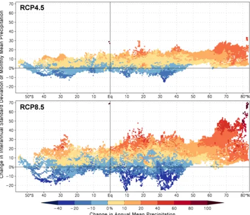
make precipitation projections more relevant, we concentrate on the relative changes between precipitation means and variability, the later quantified as the IASD of monthly precipitation. Figure 4 is a scatter diagram where the abscissa is the latitude of land grid points on the high-resolution grid used for multi-model results. The ordinate shows the change in the IASD of monthly mean precipitation from the historical case, averaged

(8)

HESSD

11, 8537–8569, 2014

Title Page

Tables Figures

◭ ◮

Back Close

Full Screen / Esc

Discussion

P

a

per

|

Discus

sion

P

a

per

|

Discussion

P

a

per

|

Discussion

P

a

per

|

over all months, to each of the two future scenarios indicated. Colors show the corre-sponding change in annual mean precipitation for each correcorre-sponding grid point.

A number of noteworthy features are evident in this figure. First, as one might expect, the range of changes in both mean precipitation and its variability are generally larger in the RCP8.5 case than in RCP4.5. Second, there is a strong correspondence between

5

the changes in mean and variance – the redder colors tend to appear for the larger changes of IASD, and the bluer colors are for the small and negative changes. North of about 50◦N, nearly all locations are projected to have increases in both the mean and variability of precipitation.

From the standpoint of impacts, the most important feature may be the

preponder-10

ance of points above thex axis that are shaded blue. These indicate locations where mean precipitation is projected to decrease, but interannual variability will increase. This is a particularly troubling combination, as it suggests both less reliability and less availability of water from precipitation sources in these locations. The extent and mag-nitude of changes of this type are greater in the RCP8.5 case. By contrast, there are

15

almost no points below thex axis that are in shades of orange or red – few locations are projected to have both more abundant and less variable precipitation.

Figure 5 shows the spatial distribution of locations that are projected to have, in the RCP8.5 case, a decrease of mean precipitation and an increase in interannual variability. Shading denotes the average change in the IASD of monthly precipitation

20

– the ordinate of Fig. 4. Locations are masked out (shaded white) where either pre-cipitation is projected to increase or variability will decrease. The shaded regions can be interpreted as areas of particular vulnerability, quantified specifically from the me-teorological sector of the water cycle. They cover more than 20 % of the land area, excluding Antarctica. Of course, regions that are projected to experience sharp

de-25

(9)

HESSD

11, 8537–8569, 2014

Title Page

Tables Figures

◭ ◮

Back Close

Full Screen / Esc

Discussion

P

a

per

|

Discus

sion

P

a

per

|

Discussion

P

a

per

|

Discussion

P

a

per

|

4.2 The agricultural sector

For the agricultural sector, we examine the projected changes in soil moisture in ar-eas where crops are grown. Figure 6 shows an example of crop data from Sacks et al. (2010) for maize. Planting and harvest date data, and thus growing season defini-tions, are primarily defined within political boundaries in this data set. The mean dates

5

are used in each case; data on the range of start and end dates are also available, but we assume that they amount to random variations that will not affect the aggregate statistics. Faint shading indicates where dates in the data set were extrapolated to fill in regions of missing data. The coverage map (upper right) is used to generate area-weighted global means of growing season mean top 10 cm soil moisture and IASD

10

(based on monthly values) for each crop.

Table 2 lists the crops in order of coverage area, as well as some basic water cycle statistics as represented by the mean of the 10 CMIP5 models investigated. Specifically shown are the area-weighted global averages of the annual mean and monthly IASD of moisture in the top 10 cm of soil for the growing season during the last 90 years of the

15

historical simulation. Also given are the weighted area averaged deviations from the historical case values for the RCP4.5 and RCP8.5 cases. There is no straightforward way to determine statistical significance, so changes of more than 3 % in both metrics are highlighted in bold.

Several features stand out. There is again a strong but not universal tendency for

20

the RCP8.5 case to show greater changes than the RCP4.5 case. Almost all area-averaged changes are negative, although maps of the changes show regions of both increasing and decreasing soil moisture in every instance. The greatest decreases for both RCP4.5 and RCP8.5 cases are for barley and sugarbeets, both primarily Euro-pean crops. Much of Europe suffers widespread precipitation decreases during

sum-25

(10)

HESSD

11, 8537–8569, 2014

Title Page

Tables Figures

◭ ◮

Back Close

Full Screen / Esc

Discussion

P

a

per

|

Discus

sion

P

a

per

|

Discussion

P

a

per

|

Discussion

P

a

per

|

existing agriculture, increases in year-to-year variations in moisture are particularly detrimental. 14 of 19 crops are projected to experience greater interannual variabil-ity of soil moisture under the RCP4.5 scenario, and 13 of 19 in the RCP8.5 case, with all increases of more than 3 % occurring in RCP8.5. The most strongly affect crops are projected to be tropical varieties: yams, sweet potato and cassava. Rice is also

5

projected to experience increases in soil moisture IASD of nearly 5 % on average in the RCP8.5 case, even though mean soil moisture changes little. Winter rye and sun-flower are forecast to have decreases of at least 3 % in both the mean and IASD of soil moisture.

To quantify further how soil moisture may change, cumulative probability distributions

10

have been calculated. The distributions are calculated spatially across the growing re-gions of each crop using the time mean soil moisture values, weighted by fractional coverage. For soil moisture, we focus on the median value and the value of the lowest decile (50 and 10 % of the cumulative distributions respectively) in the historical case, and then find what fraction of the crop areas lie below those values in the future

cli-15

mate cases. Values exceeding 50 or 10 % respectively indicate an increased area of that cropland experiencing drier conditions. 100 bins of equal range of soil moisture are used, chosen to span the range of values in each case. Results are shown in Ta-ble 3. Situations where the drier areas have increased in extent by 20 and 40 % are highlighted.

20

Again, drying is generally stronger for the RCP8.5 case. However, in terms of frac-tional increases in area, it is the dry tail of the distribution that often suffers the greatest impact. Higher latitude crops such as barley, oats, winter rye and sugarbeets show the most pronounced shifts in median soil moisture. Sunflower is also strongly affected at the dry end of the soil moisture range. Rice, sorghum, millet, cotton, rapeseed and

25

sweet potato are relatively stable in terms of their overall probability distributions of mean soil moisture.

(11)

HESSD

11, 8537–8569, 2014

Title Page

Tables Figures

◭ ◮

Back Close

Full Screen / Esc

Discussion

P

a

per

|

Discus

sion

P

a

per

|

Discussion

P

a

per

|

Discussion

P

a

per

|

changes, although tables of all these other terms are not shown here. For many of the crops, the increased area at the dry end of the distribution follows a similar decrease in rainfall at the dry tail. However, for groundnuts and particularly winter rye, there are no-table increases in precipitation and a smaller area of cultivation experiencing less than the lower decile of rainfall based on the historical values. For winter rye, there is a huge

5

increase in total evapotranspiration during the growing season, which is the main driver of soil moisture depletion. For groundnuts as well as millet, soybeans and yams, there is a notable increase in runoffat the dry end of the spectrum, consistent with change in the nature of precipitation towards fewer, more intense events. This is also evident for the shifts in the medians, where groundnuts, millet, pulses and rice show little change

10

in mean soil moisture even though they experience increases in median and mean rain-fall, with the difference going largely to increased runoff. Low-latitude crops in particu-lar experience lower median soil moisture even though median precipitation increases, because runo_ff rates also increase. Yams o_ffer an extreme example, as median pre-cipitation increases slightly, but 68 % of the crop area in the RCP8.5 case experiences

15

runoff higher than the historical median, and 57 % has lower soil moisture than the historical median. This change results in a large shift in the distribution of evapotran-spiration as well, where 86 % of the yam-growing area has lower ET than the historical median. Rapeseed has little change in median soil moisture but a positive shift in rain-fall nearly as strong as winter rye, and like winter rye the moisture sink appears to be

20

evapotranspiration.

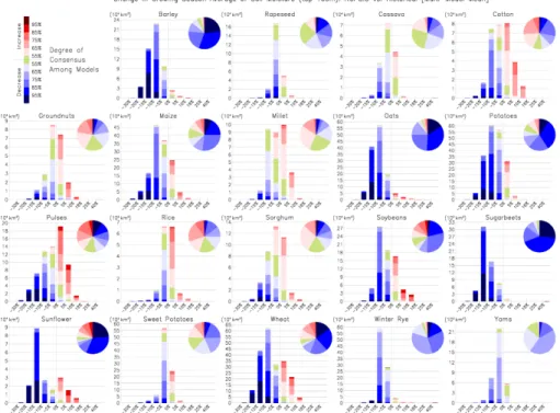
Lastly, we combine the calculation of degree of consensus among models for a pos-itive vs. negative change (cf. Dirmeyer et al., 2013, 2014) with the distribution of pro-jected soil moisture changes for each crop. Figures 7 and 8 show for each crop the total area projected to have soil moisture changes in each of 12 ranges (six positive,

25

(12)

HESSD

11, 8537–8569, 2014

Title Page

Tables Figures

◭ ◮

Back Close

Full Screen / Esc

Discussion

P

a

per

|

Discus

sion

P

a

per

|

Discussion

P

a

per

|

Discussion

P

a

per

|

have nearly complete consensus (>85 %) among the CMIP5 models for drier soils over more than half of their area. Most crops are dominated by drying soils. In the RCP4.5 case (Fig. 8) overall the impacts are less severe, the consensus for drying is somewhat weaker, and there is a greater but still subordinate indication for areas of wetter soils.

Figure 9 shows the same style of plot for the IASD – only the RCP8.5 case is shown

5

as the situation for RCP4.5 is again similar but weaker. For most crops there is a pro-jected increase in interannual variability of soil moisture, with the most severely af-fected crop being sweet potatoes. While yams and cassava also show a strong trend toward increased variability over most of their areas, rice, potatoes, and rapeseed show a greater area under a high consensus among models for increased variability. Winter

10

rye shows a majority of its area having a split vote among models (shaded green) yet a clear skew in the distribution toward decreased IASD, suggesting the multi-model results for that crop may be strongly influenced by extremes in one or two models, and uncertainty should be considered large.

4.3 The hydrological sector 15

Figure 10a shows the average simulated annual runofffor the 100 largest named river basins in the TRIP data set. On such long time scales, the runoff is effectively equal to precipitation minus evapotranspiration. Fig. 10b and c show the projected change in runoff, in percent, from historical to the RCP4.5 and RCP8.5 cases respectively. The patterns of change are largely similar but the magnitudes are generally larger for the

20

RCP8.5 case. There are projected decreases in basin-scale runo_ff in the Americas from the southern United States to the subtropical region of South America, in a band from Europe to central Asia, and across southern Africa. Other areas show increases, with the largest percentage changes over northwestern Africa, high latitudes in the Northern Hemisphere, Australia and the mid-latitudes of South America.

25

(13)

HESSD

11, 8537–8569, 2014

Title Page

Tables Figures

◭ ◮

Back Close

Full Screen / Esc

Discussion

P

a

per

|

Discus

sion

P

a

per

|

Discussion

P

a

per

|

Discussion

P

a

per

|

an increase in IASD of hydrologic metrics implies less dependability and a greater propensity for extremes. Most regions show an increase in variability, including in the RCP8.5 case many of the same areas that show a decrease in annual runoff. The greatest percentage increases are over South Asia and western Africa.

An important tendency is revealed in Fig. 11, which shows the percentage change

5

in the IASD scattered against the change in annual runoff for the 100 basins. The top panel is the change for the RCP4.5 case, and the bottom is for RCP8.5. The 12 largest basins are labeled and the sizes of the symbols are proportional to the ranks of the basins by area; colors simply help to differentiate the symbols. Many basins have a greater percentage increase in standard deviation than percentage increase in

10

mean, indicated as the points that lie within the upper grey triangles. However, very few basins show a greater decrease in standard deviation than mean (points in the lower grey triangles). This asymmetry is reflected in the best fit linear regression through the points (solid line), which crosses the 0 % mean runo_ffchange line at about₊4.6 % change in standard deviation in the RCP4.5 case, and at+5.8 % for the RCP8.5 case.

15

This mirrors, at the basin scale, what was found for precipitation at the point scale in Sect. 4.1; variability in the water cycle increases even when the mean is unchanged.

5 Discussion of caveats

There are a number of caveats that apply to this study. In all cases, estimates are calcu-lated month-by-month then averaged for seasons; they do not represent the changes

20

in seasonal totals or averages. This is a subtle distinction not expected to affect our conclusions, but the use of monthly data increases our sample size considerably and thus confidence in the statistics. Anomalies in precipitation especially are generally un-correlated from month to month. For the assessment of changes in extremes in Sect. 3, the choice of the 10 % tails is arbitrary and may not be an appropriate absolute

thresh-25

(14)

HESSD

11, 8537–8569, 2014

Title Page

Tables Figures

◭ ◮

Back Close

Full Screen / Esc

Discussion

P

a

per

|

Discus

sion

P

a

per

|

Discussion

P

a

per

|

Discussion

P

a

per

|

The estimates of the impacts of changes to the surface water cycle on agriculture are based on static contemporary crop distributions. In reality, agriculture is constantly changing and patterns of land use will adapt to changing climate as much as possible. The results on impacts to the agricultural sector should be interpreted as a measure of potential hydrologic vulnerability to various cropping areas as they are currently

dis-5

tributed. There are other climate change effects as well, notably temperature and atmo-spheric CO₂, that are not considered here but have been documented elsewhere (e.g., Rosenzweig et al., 2014). The degree of crop-level impacts in this study should be in-terpreted as a measure of likely degree of need for adaptation to maintain productivity for each crop.

10

Furthermore, the CMIP5 models do not necessarily specify the same distribution of agriculture as the crop data of Sacks et al. (2010), and none of the CMIP5 models represent as many different crop types at such high spatial resolution. This creates nu-merous local inconsistencies between the observed crop distributions we have used, and the type of vegetation specified in the climate models (as well as ever-present

in-15

consistencies between models). This is also a problem whenever climate model output is reapplied as forcing to component models (cfr. Schellnhuber et al., 2014).

The assessment of the hydrological sector neglects the effects of reservoirs, irriga-tion, and other anthropogenic controls on surface water in river basins, as these are generally not accounted for in the climate models either. Annual means are examined

20

because area-averaged runoff is not analogous to discharge on time scales shorter than one year due to lags in transport as runoffis routed through the river system. Sim-ilarly, basin aggregation smoothes out local extremes, as both drying and moistening trends are projected to occur in different parts of some of the larger river basins. Both flood control issues and the need to cache water in reservoirs to weather drought could

25

be more severe than the basin-scale results suggest.

(15)

HESSD

11, 8537–8569, 2014

Title Page

Tables Figures

◭ ◮

Back Close

Full Screen / Esc

Discussion

P

a

per

|

Discus

sion

P

a

per

|

Discussion

P

a

per

|

Discussion

P

a

per

|

climate change on different regions and facets of the meteorological, agricultural and hydrological sectors. For instance, the general conclusion is likely sound that most crops should experience drier soils and greater year-to-year variability in soil moisture, with certain crops being much more strongly affected than others. But as the spatial scale decreases, uncertainty in the projections increases.

5

6 Summary

A global examination of the projections of 10 CMIP5 climate models for RCP4.5 and RCP8.5 impacts has been conducted for the meteorological, agricultural and hydro-logical sectors, represented respectively by precipitation, soil moisture and runoff. Changes in extremes, means and interannual variability have been assessed. For the

10

agricultural and hydrologic sectors, climate change data has been convolved with data on crop distribution and river basin boundaries to provide targeted assessments.

Changes in extremes are defined by rates of exceedance of the driest and wettest 10 % thresholds derived from the historical 20th century simulations by each model at each grid point for each month of the year. For the RCP4.5 climate projection, the

15

only significant changes are towards increased drought with northern South America appearing the most vulnerable in terms of precipitation and runoff. For soil moisture, many other areas of the globe also show marked increases in drought frequency. The drought trends intensify in the RCP8.5 case, but increased rates of flood conditions also appear around the globe. There is an overall tendency for drought amplification

20

to outpace flood amplification in soil moisture, but the opposite is true for runoff. The precipitation response lies between the other two variables, with increased drought most prevalent during JJA and flooding escalating most during DJF.

Sector assessments show that for precipitation, the projected increases in interan-nual variability will be a major issue, driving the increases in extremes in all water cycle

25

(16)

HESSD

11, 8537–8569, 2014

Title Page

Tables Figures

◭ ◮

Back Close

Full Screen / Esc

Discussion

P

a

per

|

Discus

sion

P

a

per

|

Discussion

P

a

per

|

Discussion

P

a

per

|

precipitation variability and a decrease in the mean for the RCP8.5 case – a particularly dangerous combination for water resources.

In the agricultural sector, soil moisture changes in the growing areas of 19 major crops show that staples predominantly grown in Europe are likely to be hardest hit by drought. Many crops show offsetting regional impacts, although no attempt to account

5

for agricultural adaptation has been made in this study. Global crops least affected by changes in mean soil moisture are rice, groundnuts, sweet potato, pulses and cotton. However, increased interannual variability in soil moisture is projected to affect most crops, especially in tropical areas. Figures 7 and 8 provide detailed accounting of pro-jected impacts for each crop.

10

In the hydrological sector, the increase in variability of runo_ff is projected to ex-ceed the changes in the mean for most river basins, despite widespread projected the changes (usually increases) in annual mean discharge. This has major implications for flood control, as the combination suggests increased river flooding, although droughts are projected to become more likely in many basins.

15

Several of the tendencies found reflect a noteworthy aspect of the water cycle in a warming climate. Namely, precipitation is projected change toward fewer but more intense events. This change reduces overall infiltration, increases surface runoffas well as its variability. It is also a contributing factor in the overall reduction in soil moisture seen in Sect. 4.2. Thus, the change in precipitation statistics lies at the heart of both

20

the drying trend in soil moisture and the trend towards increased river basin discharge. While such results are consistent with theory and observations (e.g., Karl and Knight, 1998; Meehl et al., 2005; Donat et al., 2013), the degree to which the parameterizations in climate models properly represent the sensitivity of precipitation processes is not well known.

25

Author contributions

(17)

HESSD

11, 8537–8569, 2014

Title Page

Tables Figures

◭ ◮

Back Close

Full Screen / Esc

Discussion

P

a

per

|

Discus

sion

P

a

per

|

Discussion

P

a

per

|

Discussion

P

a

per

|

taught by the first author. Z. W. performed preliminary processing of data for all models and calculated basic statistics. G. F. calculated the decile extremes statistics in Sect. 3. P. Y. and A. M. analyzed results and provided sector-based context assessment. P. A. D. synthesized the sector-based results and prepared the manuscript with contributions from all co-authors.

5

Acknowledgements. We thank the climate modeling groups listed in Table 1 for making their model output available through the US Department of Energy’s Program for Climate Model Diagnosis and Intercomparison (PCMDI), and acknowledge the World Climate Research Pro-gramme (WCRP) Working Group on Coupled Modelling, which is responsible for CMIP5. The lead author’s synthesis of the student material was supported by joint funding from the National

10

Science Foundation (ATM-0830068), the National Oceanic and Atmospheric Administration (NA09OAR4310058), and the National Aeronautics and Space Administration (NNX09AN50G) of the Center for Ocean Land Atmosphere Studies (COLA).

References

Dankers, R., Arnell, N. W., Clark, D. B., Falloon, P. D., Fekete, B. M., Gosling, S. N., Heinke, J.,

15

Kim, H., Masaki, Y., Satoh, Y., Stacke, T., Wada, Y., and Wisser, D.: First look at changes in flood hazard in the Inter-Sectoral Impact Model Intercomparison Project ensemble, P. Natl. Acad. Sci. USA, 111, 3257–3261, doi:10.1073/pnas.1302078110, 2014.

Dirmeyer, P. A., Jin, Y., Singh, B., and Yan, X.: Trends in land–atmosphere interactions from CMIP5 simulations, J. Hydrometeorol., 14, 829–849, doi:10.1175/JHM-D-12-0107.1, 2013.

20

Dirmeyer, P. A., Wang, Z., Mbuh, M. J., and Norton, H. E.: Intensified land surface control on boundary layer growth in a changing climate, Geophys. Res. Lett., 41, 1290–1294, doi:10.1002/2013GL058826, 2014.

Donat, M. G., Alexander, L. V., Yang, H., Durre, I., Vose, R., Dunn, R. J. H., Willett, K. M., Aguilar, E., Brunet, M., Caesar, J., Hewitson, B., Jack, C., Klein Tank, A. M. G., Kruger, A.

25

(18)

HESSD

11, 8537–8569, 2014

Title Page

Tables Figures

◭ ◮

Back Close

Full Screen / Esc

Discussion

P

a

per

|

Discus

sion

P

a

per

|

Discussion

P

a

per

|

Discussion

P

a

per

|

indices since the beginning of the twentieth century: the HadEX2 data set, J. Geophys. Res., 118, 2098–2118, 2013.

Karl, T. R. and Knight, R. W.: Secular trends of precipitation amount, frequency, and intensity in the United States, B. Am. Meteorol. Soc., 79, 231–241, 1998.

Koster, R. D., Guo, Z., Dirmeyer, P. A., Yang, R., Mitchell, K., and Puma, M. J.:

5

On the nature of soil moisture in land surface models, J. Climate, 22, 4322–4335, doi:10.1175/2009JCLI2832.1, 2009.

Meehl, G. A., Arblaster, J. M., and Tebaldi, C.: Understanding future patterns of increased precipitation intensity in climate model simulations, Geophys. Res. Lett., 32, L18719, doi:10.1029/2005GL023680, 2005.

10

Oki, T., Nishimura, T., and Dirmeyer, P.: Assessment of annual runofffrom land surface models using Total RunoffIntegrating Pathways (TRIP), J. Meteorol. Soc. Jpn., 77, 235–255, 1999. Prudhomme, C., Giuntoli, I., Robinson, E. L., Clark, D. B., Arnell, N. W., Dankers, R., Fekete,

B. M., Franssen, W., Gerten, D., Gosling, S. N., Hagemann, S., Hannah, D. M., Kim, H., Masakik, Y., Satoh, Y., Stackei, T., Wada, Y., and Wisser, D.: Hydrological droughts in the

15

21st century, hotspots and uncertainties from a global multimodel ensemble experiment, P. Natl. Acad. Sci. USA, 111, 3262–3267, doi:10.1073/pnas.1222473110, 2014.

Rosenzweig, C., Elliott, J., Deryng, D., Ruane, A. C., Müller, C., Arneth, A., Boote, K. J., Fol-berth, C., Glotter, M., Khabarov, N., Neumann, K., Piontek, F., Pugh, T. A. M., Schmid, E., Stehfest, E., Yang, H., and Jones, J. W.: Assessing agricultural risks of climate change in the

20

21st century in a global gridded crop model intercomparison, P. Natl. Acad. Sci. USA, 111, 3268–3273, doi:10.1073/pnas.1222463110, 2014.

Sacks, W. J., Deryng, D., Foley, J. A., and Ramankutty, N.: Crop planting dates: an analysis of global patterns, Global Ecol. Biogeogr., 19, 607–620, doi:10.1111/j.1466-8238.2010.00551.x, 2010.

25

Schellnhuber, H. J., Frieler, K., and Kabat, P.: The elephant, the blind, and the inter-sectoral intercomparison of climate impacts, P. Natl. Acad. Sci. USA, 111, 3225–3227, doi:10.1073/pnas.1321791111, 2014.

Schewe, J., Heinke, J., Gerten, D., Haddeland, I., Arnell, N. W., Clark, D. B., Dankers, R., Eisner, S., Fekete, B. M., Colón-González, F. J., Gosling, S. N., Kim, H., Liu, X., Masaki, Y.,

30

(19)

HESSD

11, 8537–8569, 2014

Title Page

Tables Figures

◭ ◮

Back Close

Full Screen / Esc

Discussion

P

a

per

|

Discus

sion

P

a

per

|

Discussion

P

a

per

|

Discussion

P

a

per

|

climate change, P. Natl. Acad. Sci. USA, 111, 3245–3250, doi:10.1073/pnas.1222460110, 2014.

Taylor, K. E., Stouffer, R. J., and Meehl, G. A.: An overview of CMIP5 and the experiment design, B. Am. Meteorol. Soc., 93, 485–498, 2012.

van Vuuren, D. P., Edmonds, J., Kainuma, M., Riahi, K., Thomson, A., Hibbard, K., Hurtt, G. C.,

5

(20)

HESSD

11, 8537–8569, 2014

Title Page

Tables Figures

◭ ◮

Back Close

Full Screen / Esc

Discussion

P

a

per

|

Discus

sion

P

a

per

|

Discussion

P

a

per

|

Discussion

P

a

per

|

Table 1.CMIP5 models used in this paper.

Center Model Version Resolution Notes

Canadian Centre for Climate Modelling and Analysis

CanESM2 128×64

Commonwealth Scientific and Industrial Research Organisation – Bureau of Mete-orology

ACCESS1-0 192×145 No runoff data; no soil

moisture for RCP4.5

Institute for Numerical Mathematics INM-CM4 180×120

University of Tokyo Division of Climate System Research

MIROC5 256×128

Met Office Hadley Centre HadGEM2-ES 192×145 No runoffdata

Meteorological Research Institute, Japan Meteorological Agency

MRI-CGCM3 320×160

National Aeronautical and Space Administration-Goddard Institute for Space Studies

GISS-E2-R 144×90

Norwegian Climate Centre NorESM1-M 144×96

National Oceanic and Atmospheric Administration-Geophysical Fluid Dynam-ics Laboratory

GFDL-ESM2M 144×90

National Center for Atmospheric Research

(21)

HESSD

11, 8537–8569, 2014

Title Page

Tables Figures

◭ ◮

Back Close

Full Screen / Esc

Discussion

P

a

per

|

Discus

sion

P

a

per

|

Discussion

P

a

per

|

Discussion

P

a

per

|

Table 2.Crop coverage-weighted statistics of mean and interannual standard deviation (IASD) of top 10 cm soil moisture [kg m−2

] during the 20th Century (Hist.) and projected changes [%] from multi-model averages of 10 CMIP5 models. Changes of at least_±3 % are shown in bold.

Crop Type Area Mean Change Change IASD Change Change

[103km2] (Hist.) (RCP4.5) (RCP8.5) (Hist.) (RCP4.5) (RCP4.5)

Wheat 2092 20.8 −2.1 % −4.5 % 3.5 +0.1 % −1.1 %

Rice 1526 27.9 +0.4 % −0.2 % 3.3 +0.9 % +4.5 %

Maize 1361 24.9 −2.2 % −4.6 % 3.6 +1.3 % +2.6 %

Soybeans 746 25.8 −1.5 % −3.3 % 3.8 +2.0 % +3.6 %

Pulses 671 21.6 −0.5 % −1.5 % 3.3 +0.2 % +1.6 %

Barley 543 21.0 −3.3 % −8.2 % 3.3 −0.1 % −1.3 %

Sorghum 389 21.2 −0.9 % −2.7 % 3.4 +1.7 % +_{3.5 %}

Millet 334 17.7 −0.6 % −1.6 % 3.2 +0.3 % +1.8 %

Cotton 305 19.7 −0.8 % −1.2 % 3.5 +0.6 % +2.3 %

Rapeseed 246 25.4 −1.1 % −2.2 % 3.4 −0.7 % +0.1 %

Groundnuts 222 22.6 −0.1 % −0.8 % 3.5 +1.0 % +_{3.3 %}

Sunflower 204 20.2 −1.9 % −6.8 % 3.5 −0.4 % −3.0 %

Potatoes 193 24.1 −2.1 % −5.2 % 3.4 +1.8 % +2.4 %

Cassava 155 25.7 −0.8 % −2.1 % 2.8 +1.9 % +6.5 %

Oats 132 22.2 −2.8 % −7.9 % 3.5 −0.1 % −1.1 %

Winter Rye 94 28.5 −2.5 % −5.6 % 3.4 −1.1 % −4.4 %

Sweet Potato 91 26.6 −0.6 % −1.4 % 3.3 +2.7 % +7.1 %

Sugarbeets 61 21.7 −3.7 % −9.9 % 3.4 +0.9 % −1.0 %

(22)

HESSD

11, 8537–8569, 2014

Title Page

Tables Figures

◭ ◮

Back Close

Full Screen / Esc

Discussion

P

a

per

|

Discus

sion

P

a

per

|

Discussion

P

a

per

|

Discussion

P

a

per

|

Table 3.Crop coverage-weighted multi-model estimates of median (50 %) and lowest decile (10 %) values of top 10 cm soil moisture [kg m−2

] in historical case (Hist.) and the projected percentage of area that will fall below those values in two future climate scenarios. Cases where the area increases by at least 20 % (i.e., by 10 % for median, 2 % for lowest decile) are shown in bold, 40 % (20 % for median, 4 % for lowest decile) are bold and italic.

Crop Type Median Below Below Decile Below Below

(Hist.) (RCP4.5) (RCP8.5) (Hist.) (RCP4.5) (RCP4.5)

Wheat 21.0 55 % 62 % 13.5 12 % 13 %

Rice 29.6 49 % 52 % 18.9 10 % 9 %

Maize 25.1 58 % 63 % 18.5 11 % 15 %

Soybeans 25.2 59 % 62 % 21.0 11 % 15 %

Pulses 22.0 52 % 54 % 11.6 11 % 12 %

Barley 21.9 59 % 73 % _13.7 _{12 %} _{13 %}

Sorghum 21.9 53 % 56 % 12.5 10 % 11 %

Millet 16.2 51 % 52 % 10.5 11 % 11 %

Cotton 18.8 51 % 51 % 10.8 11 % 11 %

Rapeseed 28.0 49 % 54 % 13.6 11 % 10 %

Groundnuts 23.6 50 % 50 % 13.8 11 % 13 %

Sunflower 19.6 57 % 68 % 14.8 12 % 22 %

Potatoes 23.9 55 % 60 % 17.1 12 % 13 %

Cassava 26.5 51 % 55 % 19.2 12 % 14 %

Oats 22.3 62 % 75 % 17.7 13 % 19 %

Winter Rye 29.1 64 % 83 % _25.6 18 % 24 %

Sweet Potato 27.6 51 % 52 % 18.5 11 % 11 %

Sugarbeets 21.6 59 % 70 % _16.2 _{12 %} 17 %

(23)

HESSD

11, 8537–8569, 2014

Title Page

Tables Figures

◭ ◮

Back Close

Full Screen / Esc

Discussion

P

a

per

|

Discus

sion

P

a

per

|

Discussion

P

a

per

|

Discussion

P

a

per

|

(24)

HESSD

11, 8537–8569, 2014

Title Page

Tables Figures

◭ ◮

Back Close

Full Screen / Esc

Discussion

P

a

per

|

Discus

sion

P

a

per

|

Discussion

P

a

per

|

Discussion

P

a

per

|

(25)

HESSD

11, 8537–8569, 2014

Title Page

Tables Figures

◭ ◮

Back Close

Full Screen / Esc

Discussion

P

a

per

|

Discus

sion

P

a

per

|

Discussion

P

a

per

|

Discussion

P

a

per

|

(26)

HESSD

11, 8537–8569, 2014

Title Page

Tables Figures

◭ ◮

Back Close

Full Screen / Esc

Discussion

P

a

per

|

Discus

sion

P

a

per

|

Discussion

P

a

per

|

Discussion

P

a

per

|

(27)

HESSD

11, 8537–8569, 2014

Title Page

Tables Figures

◭ ◮

Back Close

Full Screen / Esc

Discussion

P

a

per

|

Discus

sion

P

a

per

|

Discussion

P

a

per

|

Discussion

P

a

per

|

(28)

HESSD

11, 8537–8569, 2014

Title Page

Tables Figures

◭ ◮

Back Close

Full Screen / Esc

Discussion

P

a

per

|

Discus

sion

P

a

per

|

Discussion

P

a

per

|

Discussion

P

a

per

|

Figure 6.Mean planting and harvest dates (indicated by month), total length of growing season (days) and the fractional coverage of each 1/12◦

(29)

HESSD

11, 8537–8569, 2014

Title Page

Tables Figures

◭ ◮

Back Close

Full Screen / Esc

Discussion

P

a

per

|

Discus

sion

P

a

per

|

Discussion

P

a

per

|

Discussion

P

a

per

|

(30)

HESSD

11, 8537–8569, 2014

Title Page

Tables Figures

◭ ◮

Back Close

Full Screen / Esc

Discussion

P

a

per

|

Discus

sion

P

a

per

|

Discussion

P

a

per

|

Discussion

P

a

per

|

(31)

HESSD

11, 8537–8569, 2014

Title Page

Tables Figures

◭ ◮

Back Close

Full Screen / Esc

Discussion

P

a

per

|

Discus

sion

P

a

per

|

Discussion

P

a

per

|

Discussion

P

a

per

|

(32)

HESSD

11, 8537–8569, 2014

Title Page

Tables Figures

◭ ◮

Back Close

Full Screen / Esc

Discussion

P

a

per

|

Discus

sion

P

a

per

|

Discussion

P

a

per

|

Discussion

P

a

per

|

1

2

3

4

5

6

7

8

9

10

11

Figure 10. (a)Annual average runoff(kg m−2

(33)

HESSD

11, 8537–8569, 2014

Title Page

Tables Figures

◭ ◮

Back Close

Full Screen / Esc

Discussion

P

a

per

|

Discus

sion

P

a

per

|

Discussion

P

a

per

|

Discussion

P

a

per

|